Purdue e-Pubs
Open Access Dissertations Theses and Dissertations
Spring 2015
Stability of machine learning algorithms
Wei Sun
Purdue UniversityFollow this and additional works at:https://docs.lib.purdue.edu/open_access_dissertations
Part of theComputer Sciences Commons, and theStatistics and Probability Commons
This document has been made available through Purdue e-Pubs, a service of the Purdue University Libraries. Please contact [email protected] for additional information.
Recommended Citation
Sun, Wei, "Stability of machine learning algorithms" (2015).Open Access Dissertations. 563.
PURDUE UNIVERSITY GRADUATE SCHOOL Thesis/Dissertation Acceptance
This is to certify that the thesis/dissertation prepared By
Entitled
For the degree of
Is approved by the final examining committee:
To the best of my knowledge and as understood by the student in the Thesis/Dissertation Agreement, Publication Delay, and Certification Disclaimer (Graduate School Form 32), this thesis/dissertation adheres to the provisions of Purdue University’s “Policy of Integrity in Research” and the use of copyright material.
Approved by Major Professor(s):
Approved by:
Head of the Departmental Graduate Program Date
Wei Sun
STABILITY OF MACHINE LEARNING ALGORITHMS
Doctor of Philosophy
Guang Cheng Lingsong Zhang
Chair
Jayanta K. Ghosh
Xiao Wang
Mark Daniel Ward
Guang Cheng
A Dissertation Submitted to the Faculty
of
Purdue University by
Wei Sun
In Partial Fulfillment of the Requirements for the Degree
of
Doctor of Philosophy
May 2015 Purdue University West Lafayette, Indiana
ACKNOWLEDGMENTS
First and foremost, I would like to extend my sincerest thank to my advisor, Professor Guang Cheng for his brilliant guidance and inspirational advice. It has been the most valuable and rewarding experience working with him. As an advisor, Guang gives me enough freedom to pursue my research interests in machine learning. He has also provided numerous opportunities for me to attend meetings and collaborate with faculties from other Universities. He has been not only my advisor, but my role model as a diligent researcher to pursue important and deep topics. As a friend, he has been listening to my heart and helping me. He has been and will continue to be a source of wisdom in my life! Thanks for being a fantastic advisor and friend.
I would also like to express my great gratitude to my collaborators. I am especially indebted to Professor Junhui Wang for opening the door for me to the world of machine learning. It was a great pleasure to work with Professor Yufeng Liu at UNC, who has strongly supported every step I took in the graduate school. I thank Professor Xingye Qiao from Binghamton University for his valuable suggestions and helpful discussions on my thesis. I was very lucky to work with extremely intelligent and hard-working people at Princeton University, namely Zhaoran Wang, Junwei Lu, and Professor Han Liu. Thank Professor Yixin Fang at NYU for many valuable discussions. I also give many thanks to Pengyuan Wang and Dawei Yin at Yahoo! labs for the enjoyable collaborations during my summer internship.
On the other hand, I deeply appreciate the guidance I have received from profes-sors at Purdue University. Especially, I wish to thank Professor Jayanta K. Ghosh for his helpful comments on teaching during the period when I was a TA for his STAT528 course. Many thanks go to Professor Xiao Wang for the fruitful discussions on deep learning and Professor Lingsong Zhang, Professor Mark Ward for serving on my com-mittee and giving me invaluable comments to improve the thesis. Special thanks go
to Professor Rebecca W. Doerge for her numerous supports on my academic travels and various award applications. Furthermore, I thank Professors William S. Cleve-land, Jose Figueroa-Lopez, Sergey Kirshner, Chuanhai Liu, Yuan (Alan) Qi, Thomas Sellke for inspirational lectures that help a lot in my daily research.
I would like to acknowledge group members of Professor Guang Cheng’s research group, including Professor Shenchun Kong, Professor Qifan Song, Dr. Zuofeng Shang, Zhuqing Yu, Ching-Wei Cheng, Meimei Liu, and Botao Hao for many valuable dis-cussions on research problems over the past four years.
I also deeply appreciate generous helps from friends at Purdue. Fishing with Qiming Huang and Whitney Huang was a lot of fun. I also enjoyed a lot when we played cards during fun nights with Longjie Cheng, Xian He, Cheng Li, Chao Pan, Qiming Huang, and Bingrou (Alice) Zhou. I would also like to thank Yongheng Zhang and Xia Huang. It was great time to have fun with Terrence. Without the happiness brought to me by my friends, my life as a PhD student at West Lafayette would be miserable without a doubt.
Finally, I would like to express my heartfelt gratitude to my family, especially to my wife, whose love and support has been the driving force of my journey.
TABLE OF CONTENTS
Page
LIST OF TABLES . . . vii
LIST OF FIGURES . . . viii
ABBREVIATIONS . . . x
ABSTRACT . . . xi
1 Introduction . . . 1
1.1 Decision Boundary Instability (DBI) . . . 3
1.2 Classification Instability (CIS) . . . 4
2 Decision Boundary Instability . . . 5
2.1 Large-Margin Classifiers . . . 7
2.2 Classifier Selection Algorithm . . . 8
2.2.1 Stage 1: Initial Screening via GE . . . 8
2.2.2 Stage 2: Final Selection via DBI. . . 12
2.2.3 Relationship of DBI with Other Variability Measures . . . . 16
2.2.4 Summary of Classifier Selection Algorithm . . . 17
2.3 Large-Margin Unified Machines . . . 18
2.4 Selection Consistency . . . 20 2.5 Experiments . . . 22 2.5.1 Illustration . . . 23 2.5.2 Simulations . . . 24 2.5.3 Real Examples . . . 26 2.6 Nonlinear Extension . . . 28 2.7 Technical Proofs . . . 31 2.7.1 Proof of Theorem 2.2.1: . . . 31 2.7.2 Proof of Theorem 2.2.2 . . . 33
2.7.3 Calculation of the Transformation Matrix in Section 2.2.2. . 34
2.7.4 Approximation of DBI . . . 35
2.7.5 Proof of Corollary 1 . . . 36
2.7.6 Proof of Corollary 2 . . . 40
2.7.7 Proof of Lemma 1. . . 41
2.7.8 Proof of Theorem 2.4.1 . . . 42
3 Stabilized Nearest Neighbor Classifier and Its Theoretical Properties . . . 49
3.1 Classification Instability . . . 52
Page
3.2.1 Review of WNN. . . 53
3.2.2 Asymptotically Equivalent Formulation of CIS . . . 55
3.2.3 Stabilized Nearest Neighbor Classifier . . . 57
3.3 Theoretical Properties . . . 58
3.3.1 A Sharp Rate of CIS . . . 58
3.3.2 Optimal Convergence Rates of SNN . . . 61
3.4 Asymptotic Comparisons . . . 62
3.4.1 CIS Comparison of Existing Methods . . . 62
3.4.2 Comparisons between SNN and OWNN. . . 64
3.5 Tuning Parameter Selection . . . 66
3.6 Numerical Studies. . . 68
3.6.1 Validation of Asymptotically Equivalent Forms . . . 69
3.6.2 Simulations . . . 71 3.6.3 Real Examples . . . 74 3.7 Technical Proofs . . . 76 3.7.1 Proof of Theorem 3.2.1 . . . 76 3.7.2 Proof of Theorem 3.2.2 . . . 82 3.7.3 Proof of Theorem 3.3.1 . . . 84 3.7.4 Proof of Theorem 3.3.2 . . . 85 3.7.5 Proof of Theorem 3.3.3 . . . 89 3.7.6 Proof of Corollary 3 . . . 90
3.7.7 Proof of Corollaries 4 and 5 . . . 91
3.7.8 Calculation of B1 in Section 3.6.2 . . . 91
4 Summary . . . 93
REFERENCES . . . 95
LIST OF TABLES
Table Page
2.1 The averaged test errors and averaged test DBIs (multiplied by 100) of all methods: “cv+varcv” is the two-stage approach which selects the loss with the minimal variance of the K-CV error in Stage 2; “cv+be” is the two-stage approach which in Stage 2 selects the loss with the minimal classification stability defined in Bousquet and Elisseeff (2002); “cv+dbi” is our method. The smallest value in each case is given in bold. Standard errors are given in subscript. . . 27 2.2 The averaged test errors and averaged test DBIs of all methods in real
example. The smallest value in each case is given in bold. Standard errors are given in subscript. . . 28
LIST OF FIGURES
Figure Page
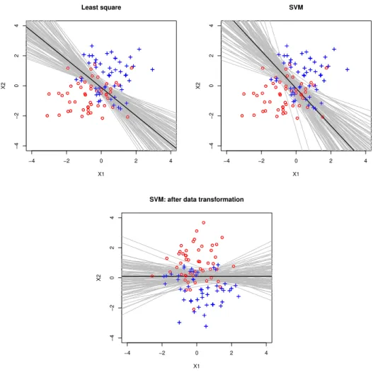
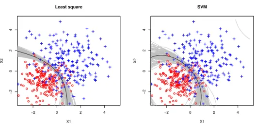
2.1 Two classes are shown in red circles and blue crosses. The black line is the decision boundary based on the original training sample, and the gray lines are 100 decision boundaries based on perturbed samples. The top left (right) panel corresponds to the least square loss (SVM). The perturbed decision boundaries of SVM after data transformation are shown in the bottom. . . 14 2.2 Plots of least square, exponential, logistic, and LUM loss functions with
γ = 0,0.5,1. . . 19 2.3 Comparison of true and estimated DBIs in Example 6.1 is shown in the left
plot. The true DBIs are denoted as red triangles and the estimated DBIs from replicated experiments are illustrated by box plots. The sensitivity of confidence level α to the proportion of potentially good classifiers in Stage 1 is shown on the right. . . 24 2.4 The K-CV error, the DBI estimate, and the perturbed decision boundaries
in Simulation 1 with flipping rate 15%. The minimal K-CV error and minimal DBI estimate are indicated with red triangles. The labels Ls, Exp, Logit, LUM0, LUM0.5, and LUM1 refer to least squares loss, exponential loss, logistic loss, and LUM loss with index γ = 0,0.5,1, respectively. . 26 2.5 The nonlinear perturbed decision boundaries for the least squares loss
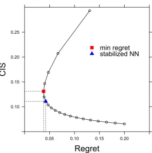
(left) and SVM (right) in the bivariate normal example with unequal vari-ances. . . 30 3.1 Regret and CIS of the kNN classifier. From top to bottom, each circle
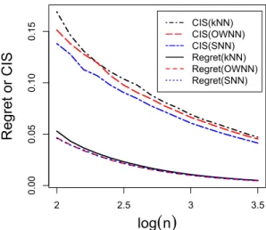
represents the kNN classifier with k ∈ {1,2, . . . ,20}. The red square corresponds to the classifier with the minimal regret and the classifier depicted by the blue triangle improves it to have a lower CIS. . . 50 3.2 Regret and CIS of kNN, OWNN, and SNN procedures for a bivariate
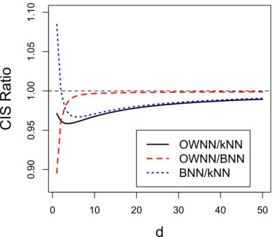
normal example. The top three lines represent CIS’s ofkNN, OWNN, and SNN. The bottom three lines represent regrets ofkNN, SNN, and OWNN. The sample size shown on the x-axis is in the log10 scale. . . 51 3.3 Pairwise CIS ratios between kNN, BNN and OWNN for different feature
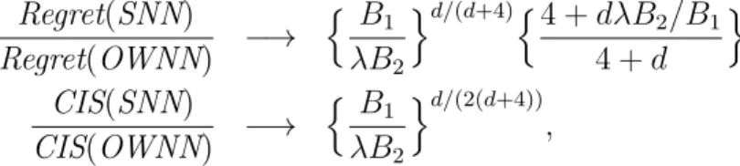
Figure Page 3.4 Regret ratio and CIS ratio of SNN over OWNN as functions of B1 and d.
The darker the color, the larger the value. . . 66 3.5 Logarithm of relative gain of SNN over OWNN as a function of B1 and
d when λ0 = 1. The grey (white) color represents the case where the
logarithm of relative gain is greater (less) than 0. . . 67 3.6 Asymptotic CIS (red curve) and estimated CIS (box plots over 100
simu-lations) for OWNN (left) and SNN (right) procedures. These plots show that the estimated CIS converges to its asymptotic equivalent value as n
increases. . . 70 3.7 Asymptotic risk (regret + the Bayes risk; red curves) and estimated risk
(black box plots) for OWNN (left) and SNN procedures (right). The blue horizontal line indicates the Bayes risk, 0.215. These plots show that the estimated risk converges to its asymptotic version (and also the Bayes risk) as n increases. . . 71 3.8 Average test errors and CIS’s (with standard error bar marked) of the
kNN, BNN, OWNN, and SNN methods in Simulation 1. The x-axis in-dicates different settings with various dimensions. Within each setting, the four methods are horizontally lined up (from the left are kNN, BNN, OWNN, and SNN). . . 72 3.9 Average test errors and CIS’s (with standard error bar marked) of the
kNN, BNN, OWNN, and SNN methods in Simulation 2. The ticks on the
x-axis indicate the dimensions and prior class probability π for different settings. Within each setting, the four methods are horizontally lined up (from the left are kNN, BNN, OWNN, and SNN). . . 73 3.10 Average test errors and CIS’s (with standard error bar marked) of the
kNN, BNN, OWNN, and SNN methods in Simulation 3. The ticks on the
x-axis indicate the dimensions and prior class probability π for different settings. Within each setting, the four methods are horizontally lined up (from the left are kNN, BNN, OWNN, and SNN). . . 74 3.11 Average test errors and CIS’s (with standard error bar marked) of the
kNN, BNN, OWNN and SNN methods for four data examples. The ticks on the x-axis indicate the names of the examples. Within each example, the four methods are horizontally lined up (from the left are kNN, BNN, OWNN, and SNN). . . 75
ABBREVIATIONS
BNN Bagged Nearest Neighbor Classifier CIS Classification Instability
DBI Decision Boundary Instability GE Generalization Error
kNN k Nearest Neighbor Classifier
OWNN Optimal Weighted Nearest Neighbor Classifier SNN Stabilized Nearest Neighbor Classifier
ABSTRACT
Sun, Wei PhD, Purdue University, May 2015. Stability of Machine Learning Algo-rithms. Major Professor: Guang Cheng.
In the literature, the predictive accuracy is often the primary criterion for evaluat-ing a learnevaluat-ing algorithm. In this thesis, I will introduce novel concepts of stability into the machine learning community. A learning algorithm is said to be stable if it pro-duces consistent predictions with respect to small perturbation of training samples. Stability is an important aspect of a learning procedure because unstable predictions can potentially reduce users’ trust in the system and also harm the reproducibility of scientific conclusions. As a prototypical example, stability of the classification proce-dure will be discussed extensively. In particular, I will present two new concepts of classification stability.
The first one is the decision boundary instability (DBI) which measures the vari-ability of linear decision boundaries generated from homogenous training samples. Incorporating DBI with the generalization error (GE), we propose a two-stage algo-rithm for selecting themost accurate and stable classifier. The proposed classifier se-lection method introduces the statistical inference thinking into the machine learning society. Our selection method is shown to be consistent in the sense that the optimal classifier simultaneously achieves the minimal GE and the minimal DBI. Various sim-ulations and real examples further demonstrate the superiority of our method over several alternative approaches.
The second one is the classification instability (CIS). CIS is a general measure of stability and generalizes DBI to nonlinear classifiers. This allows us to establish a sharp convergence rate of CIS for general plug-in classifiers under a low-noise con-dition. As one of the simplest plug-in classifiers, the nearest neighbor classifier is
extensively studied. Motivated by an asymptotic expansion formula of the CIS of the weighted nearest neighbor classifier, we propose a new classifier called stabilized nearest neighbor (SNN) classifier. Our theoretical developments further push the frontier of statistical theory in machine learning. In particular, we prove that SNN attains the minimax optimal convergence rate in the risk, and the established sharp convergence rate in CIS. Extensive simulation and real experiments demonstrate that SNN achieves a considerable improvement in stability over existing classifiers with no sacrifice of predictive accuracy.
1. INTRODUCTION
The predictive accuracy is often the primary criterion for evaluating a machine learn-ing algorithm. Recently, researchers have started to explore alternative measures to evaluate the performance of a learning algorithm. For instance, besides prediction ac-curacy, computational complexity, robustness, interpretability, and variable selection performance have been considered in the literature. Our work follows this research line since we believe there are other critical properties (other than accuracy) of a machine learning algorithm that have been overlooked in the research community. In this thesis, I will introduce novel concepts of stability into the machine learning com-munity. A learning algorithm is said to be stable if it produces consistent predictions with respect to small perturbation of training samples.
Stability is an important aspect of a learning algorithm. Data analyses have become a driving force for much scientific research work. As datasets get bigger and analysis methods become more complex, the need for reproducibility has increased significantly [1]. Many experiments are being conducted and conclusions are being made with the aid of statistical analyses. Those with great potential impacts must be scrutinized before being accepted. An initial scrutiny involves reproducing the result. A minimal requirement is that one can reach the same conclusion by applying the described analyses to the same data, a notion some refer to as replicability. A more general requirement is that one can reach a similar result based on independently generated datasets. The issue of reproducibility has drawn much attention in statistics [2], biostatistics [3, 4], computational science [5] and other scientific communities [6]. Recent discussions can be found in a special issue of Nature1). Moreover, Marcia McNutt, the Editor-in-Chief ofScience, pointed out that “reproducing an experiment is one important approach that scientists use to gain confidence in their conclusions.” 1at http://www.nature.com/nature/focus/reproducibility/
That is, if conclusions can not be reproduced, the credit of the researchers, along with the scientific conclusions themselves, will be in jeopardy.
Throughout the whole scientific research process, there are many ways statistics as a subject can help improve reproducibility. One particular aspect we stress in this thesis is the stability of the statistical procedure used in the analysis. According to [2], scientific conclusions should be stable with respect to small perturbation of data. The danger of an unstable statistical method is that a correct scientific conclusion may not be recognized and could be falsely discredited, simply because an unstable statistical method was used.
Moreover, stability can be very important in some practical domains. Customers often evaluate a service based on their experience for a small sample, where the accu-racy is either hard to perceive (due to the lack of ground truth), or does not appear to differ between different services (due to data inadequacy); on the other hand, stability is often more perceptible and hence can be an important criterion. For example, In-ternet streaming service provider Netflix has a movie recommendation system based on complex learning algorithms. Viewers either can not promptly perceive the inac-curacy because they themselves do not know which film is the best for them, or are quite tolerable even if a sub-optimal recommendation is given. However, if two con-secutively recommended movies are from two totally different genres, the customer can immediately perceive such instability, and have a bad user experience with the service. Furthermore, providing a stable prediction plays a crucial role on users’ trust of the classification system. In the psychology literature, it has been shown that advice-giving agents with a lager variability in past opinions are considered less infor-mative and less helpful than those with a more consistent pattern of opinions [7, 8]. Therefore, a machine learning system may be distrusted by users if it generates highly unstable predictions simply due to the randomness of training samples.
It is worth mentioning that stability has indeed received much attention in statis-tics. For example, in clustering problems, [9] introduced the clustering instability to assess the quality of a clustering algorithm; [10] used the clustering instability as a
criterion to select the number of clusters. In high-dimensional regression, [11] and [12] proposed stability selection procedures for variable selection, and [13] and [14] applied stability for tuning parameter selection. For more applications, see the use of sta-bility in model selection [15], analyzing the effect of bagging [16], and deriving the generalization error bound [17, 18]. However, many of these works view stability as a tool for other purposes. In literature, few work has emphasized the importance of stability itself.
As a prototypical example, in this thesis we will discuss extensively the stability of a classification procedure. Classification aims to identify the class label of a new subject using a classifier constructed from training data whose class memberships are given. It has been widely used in diverse fields, e.g., medical diagnosis, fraud detection, and computer vision. In the literature, much of the research focuses on im-proving the accuracy of classifiers. Recently, alternative criteria have been explored, such as computational complexity and training time [19], the robustness [20], among others. Our work focuses on another critical property of classifiers, namely stabil-ity, that has been somewhat overlooked. A classification procedure with more stable prediction performance is preferred when researchers aim to reproduce the reported results from randomly generated samples. Consequently, aside from high prediction accuracy, high stability is another crucial factor to consider when evaluating the per-formance of a classification procedure. Our work tries to fill this gap by presenting two new concepts of classification stability.
1.1 Decision Boundary Instability (DBI)
In Section 2, I will introduce the decision boundary instability (DBI) to capture the variability of decision boundaries arose from homogenous training samples. Incor-porating DBI with the generalization error (GE), we propose a two-stage algorithm for selecting the most accurate and stable classifier: Stage (i) eliminate the classifiers whose GEs are significantly larger than the minimal one among all the candidate
classifiers; Stage (ii) select the optimal classifier as that with the most stable deci-sion boundary, i.e., the minimal DBI, among the remaining classifiers. Our selection method is shown to be consistent in the sense that the optimal classifier simultane-ously achieves the minimal GE and the minimal DBI. Various simulations and real examples further demonstrate the superiority of our method over several alternative approaches.
1.2 Classification Instability (CIS)
In Section 3, I will introduce the classification instability (CIS) which character-izes the sampling variability of the yielded prediction. CIS is a general measure of stability for both linear and nonlinear classifiers. This allows us to establish a sharp convergence rate of CIS for general plug-in classifiers under a low-noise condition. This sharp rate is slower than but approaching n−1, which is shown by adapting the
theoretical framework of [21]. As one of the simplest plug-in classifiers, the nearest neighbor classifier is extensively studied. An important result we find is that the CIS of a weighted nearest neighbor (WNN) classifier procedure is asymptotically propor-tional to the Euclidean norm of the weight vector. This rather concise form allows us to propose a new classifier called stabilized nearest neighbor (SNN) classifier, which is the optimal solution by minimizing the CIS of a WNN procedure over an accept-able region of the weight where the regret is small. In theory, we prove that SNN attains the minimax optimal convergence rate in the risk, and the established sharp convergence rate in CIS. Extensive simulation and real experiments demonstrate that SNN achieves a considerable improvement in stability over existing classifiers with no sacrifice of predictive accuracy.
2. DECISION BOUNDARY INSTABILITY
Classification aims to identify the class label of a new subject using a classifier con-structed from training data whose class memberships are given. It has been widely used in diverse fields, e.g., medical diagnosis, fraud detection, and natural language processing. Numerous classification methods have been successfully developed with classical approaches such as Fisher’s linear discriminant analysis (LDA), quadratic discriminant analysis (QDA), and logistic regression [22], and modern approaches such as support vector machine (SVM) [23], boosting [24], distance weighted dis-crimination (DWD) [25], classification based on the reject option [26], and optimal weighted nearest neighbor classifiers [27]. In a recent paper, [28] proposed a platform, large-margin unified machines (LUM), for unifying various large margin classifiers ranging from soft to hard.
In the literature, much of the research has focused on improving the predictive ac-curacy of classifiers and hence generalization error (GE) is often the primary criterion for selecting the optimal one from the rich pool of existing classifiers; see [29] and [30]. Recently, researchers have started to explore alternative measures to evaluate the performance of classifiers. For instance, besides prediction accuracy, computational complexity and training time of classifiers are considered in [19]. Moreover, [20] pro-posed the robust truncated hinge loss SVM to improve the robustness of the standard SVM. [31] and [32] investigated several measures of cost-sensitive weighted general-ization errors for highly unbalanced classification tasks since, in this case, GE itself is not very informative. Our work follows this research line since we believe there are other critical properties (other than accuracy) of classifiers that have been overlooked in the research community. In this article, we introduce a notion of decision bound-ary instability (DBI) to assess the stability [15] of a classification procedure arising
from the randomness of training samples. Aside from high prediction accuracy, high stability is another crucial factor to consider in the classifier selection.
In this paper, we attempt to select themost accurate and stableclassifier by incor-porating DBI into our selection process. Specifically, we suggest a two-stage selection procedure: (i) eliminate the classifiers whose GEs are significantly larger than the minimal one among all the candidate classifiers; (ii) select the optimal classifier as that with the most stable decision boundary, i.e., the minimal DBI, among the re-maining classifiers. In the first stage, we show that the cross-validation estimator for the difference of GEs induced from two large-margin classifiers asymptotically follows a Gaussian distribution, which enables us to construct a confidence interval for the GE difference. If this confidence interval contains 0, these two classifiers are consid-ered indistinguishable in terms of GE. By applying the above approach, we can obtain a collection of potentially good classifiers whose GEs are close enough to the minimal value. The uncertainty quantification of the cross-validation estimator is crucially important considering that only limited samples are available in practice. In fact, experiments indicate that for certain problems many classifiers do not significantly differ in their estimated GEs, and the corresponding absolute differences are mainly due to random noise.
A natural follow-up question is whether the collection of potentially good classifiers also perform well in terms of their stability. Interestingly, we observe that the decision boundary generated by the classifier with the minimal GE estimator sometimes has unstable behavior given a small perturbation of the training samples. This observation motivates us to propose a further selection criterion in the second stage: DBI. This new measure can precisely reflect the visual variability in the decision boundaries due to the perturbed training samples.
Our two-stage selection algorithm is shown to be consistent in the sense that the selected optimal classifier simultaneously achieves the minimal GE and the minimal DBI. The proof is nontrivial because of the stochastic nature of the two-stage al-gorithm. Note that our method is distinguished from the bias-variance analysis in
classification since the latter focuses on the decomposition of GE, e.g., [33]. Our DBI is also conceptually different from the stability-oriented measure introduced in [17], which was defined as the maximal difference of the decision functions trained from the original datasets and the leave-one-out datasets. In addition, their variability measure suffers from the transformation variant issue since a scale transformation of the decision function coefficients will greatly affect their variability measure. Our DBI overcomes this problem via a rescaling scheme since DBI can be viewed as a weighted version of the asymptotic variance of the decision function. In the end, extensive experiments illustrate the advantage of our selection algorithm compared with the alternative approaches in terms of both classification accuracy and stability.
2.1 Large-Margin Classifiers
This section briefly reviews large-margin classifiers, which serve as prototypical examples to illustrate our two-stage classifier selection technique.
Let (X, Y) ∈ Rd × {1,−1} be random variables from an underlying
distribu-tion P(X, Y). Denote the conditional probability of class Y = 1 given X = x as
p(x) = P(Y = 1|X = x), where p(x) ∈ (0,1) to exclude the degenerate case. Let the input variable be x = (x1, . . . , xd)T, ˜x = (1, x1, . . . , xd)T, with coefficient w =
(w1, . . . , wd)T and parameterθ = (b,wT)T. The linear decision function is defined as
f(x;θ) =b+xTw = ˜xTθ, and the decision boundary isS(x;θ) = {x:f(x;θ) = 0}. The performance of the classifier sign{f(x;θ)} is measured by the classification risk
E[I{Y6=sign{f(X;θ)}}], where the expectation is with respect to P(X, Y). Since the di-rect minimization of the above risk is NP hard [34], various convex surrogate loss functionsL(·) have been proposed to deal with this computational issue. Denote the surrogate risk as RL(θ) =E[L(Y f(X;θ))], and assume that the minimizer ofRL(θ)
Given the training sample Dn = {(xi, yi);i = 1, . . . , n} drawn from P(X, Y), a
large-margin classifier minimizes the empirical risk OnL(θ) defined as
OnL(θ) = 1 n n X i=1 Lyi(wTxi+b) + λn 2 w Tw, (2.1)
where λn is some positive tuning parameter. The estimator minimizing OnL(θ) is
denoted asbθL= (bbL,wb
T
L)T. Common large-margin classifiers include the squared loss
L(u) = (1−u)2, the exponential lossL(u) = e−u, the logistic lossL(u) = log(1 +e−u),
and the hinge loss L(u) = (1−u)+. Unfortunately, there seems to be no general
guideline for selecting these loss functions in practice except the cross validation error. Ideally if we had access to an arbitrarily large test set, we would just choose the classifier for which the test error is the smallest. However, in reality where only limited samples are available, the commonly used cross validation error may not be able to accurately approximate the testing error. The main goal of this paper is to establish a practically useful selection criterion by incorporating DBI with the cross validation error.
2.2 Classifier Selection Algorithm
In this section, we propose a two-stage classifier selection algorithm: (i) we se-lect candidate classifiers whose estimated GEs are relatively small; (ii) the optimal classifier is that with the minimal DBI among those selected in Stage (i).
2.2.1 Stage 1: Initial Screening via GE
In this subsection, we show that the difference of the cross-validation errors ob-tained from two large-margin classifiers asymptotically follows a Gaussian distribu-tion, which enables us to construct a confidence interval for their GE difference. We further propose a perturbation-based resampling approach to construct this confi-dence interval.
Given a new input (X0, Y0) from P(X, Y), we define the GE induced by the loss
function L as
D0L=
1
2E|Y0−sign{f(X0;θbL)}|, (2.2) where bθL is based on the training sample Dn, and the expectation is with respect to
both Dn and (X0, Y0). In practice, the GE, which depends on the underlying
distri-bution P(X, Y), needs to be estimated using Dn. One possible estimate is the
em-pirical generalization error defined as DbL≡ Db(bθL), whereDb(θ) = (2n)−1
Pn
i=1|yi−
sign{f(xi;θ)}|. However, the above estimate suffers from the problem of
overfit-ting [35]. Hence, one can use the K-fold cross-validation procedure to estimate the GE; this can significantly reduce the bias [36]. Specifically, we randomly split Dn
into K disjoint subgroups and denote the kth subgroup as Ik. For k = 1, . . . , K, we
obtain the estimator bθL(−k) from all the data except those in Ik, and calculate the
empirical average Db(bθL(−k)) based only on Ik, i.e., Db(bθL(−k)) = (2|Ik|)−1
P
i∈Ik|yi−
sign{f(xi;θbL(−k))}| with |Ik| being the cardinality of Ik. The K-fold cross-validation
(K-CV) error is thus computed as
b DL=K−1 K X k=1 b D(bθL(−k)). (2.3)
We set K = 5 for our numerical experiments.
We establish the asymptotic normality of the K-CV errorDbL under the following
regularity conditions:
(L1) The probability distribution function ofX and the conditional probabilityp(x) are both continuously differentiable.
(L2) The parameter θ0L is bounded and unique.
(L3) The map θ 7→L(yf(x;θ)) is convex.
(L4) The mapθ 7→L(yf(x;θ)) is differentiable atθ=θ0La.s.. Furthermore,G(θ0L)
is element-wisely bounded, where
G(θ0L) =E h OθL(Y f(X;θ))OθL(Y f(X;θ))T i θ=θ0L .
(L5) The surrogate risk RL(θ) is bounded and twice differentiable at θ =θ0L with
the positive definite Hessian matrix H(θ0L) =O2θRL(θ)|θ=θ0L.
Assumption (L1) ensures that the GE is continuously differentiable with respect to
θ so that the uniform law of large numbers can be applied. Assumption (L3) ensures that the uniform convergence theorem for convex functions [37] can be applied, and it is satisfied by all the large-margin loss functions considered in this paper. As-sumptions (L4) and (L5) are required to obtain the local quadratic approximation to the surrogate risk function around θ0L. Assumptions (L2)–(L5) were previously used
by [38] to prove the asymptotic normality of bθL.
Theorem 2.2.1 below establishes the asymptotic normality of the K-CV error DbL
for any large-margin classifier, which generalizes the result for the SVM in [36].
Theorem 2.2.1 Suppose Assumptions (L1)–(L5) hold and λn =o(n−1/2). Then for any fixed K, WL= √ nDbL−D0L d −→N0, E(ψ12) as n→ ∞, (2.4) where ψ1 = 12|Y1−sign{f(X1;θ0L)}| −D0L−d˙(θ0L)TH(θ0L)−1M1(θ0L) with d˙(θ) =
OθE(Db(θ)), and M1(θ) =OθL(Y1f(X1;θ)).
An immediate application of Theorem 2.2.1 is to compare two competing classifiers
L1 and L2. Define their GE difference ∆12 and its consistent estimate ∆b12 to be
D02−D01andDb2−Db1, respectively. To test whether the GEs induced byL1andL2 are
significantly different, we need to establish an approximate confidence interval for ∆12
based on the distribution ofW∆12 ≡ W2−W1 =n
1/2(
b
∆12−∆12). In practice, we apply
the perturbation-based resampling procedure [39] to approximate the distribution of W∆12. This procedure was also employed by [36] to construct the confidence interval
of SVM’s GE. Specifically, let {Gi}ni=1 be i.i.d. random variables drawn from the
exponential distribution with unit mean and unit variance. Denote
b θ∗j = arg min b,w ( 1 n n X i=1 GiLj yi(wTxi+b) +λn 2 w Tw ) . (2.5)
Conditionally on Dn, the randomness of bθ
∗
j merely comes from that of G1, . . . , Gn.
Denote W∆∗ 12 =W ∗ 2 −W ∗ 1 with Wj∗ =n−1/2 n X i=1 n1 2 yi−sign{f(xi,θb ∗ j)} −Dbj o Gi. (2.6)
By repeatedly generating a set of random variables {Gi, i= 1, . . . , n}, we can obtain
a large number of realizations of W∆∗
12 to approximate the distribution of W∆12. In
Theorem 2.2.2 below, we prove that this approximation is valid.
Theorem 2.2.2 Suppose the assumptions in Theorem 2.2.1 hold, we have W∆12
d
−→N0, V ar(ψ12−ψ11)
,
as n → ∞, where ψ11 and ψ12 are defined in Appendix A.3, and
W∆∗12 =d⇒N0, V ar(ψ12−ψ11)
conditional on Dn,
where “=⇒” means conditional weak convergence in the sense of [40].
Algorithm 1below summarizes the resampling procedure for establishing the
con-fidence interval of the GE difference ∆12.
Algorithm 1 (Generalization Error Comparison Algorithm)
Input: Training sampleDn and two candidate classifiersL1 and L2.
• Step 1. Calculate K-CV errorsDb1 and Db2 of classifiers L1 and L2, respectively.
• Step 2. For r= 1, . . . , N, repeat the following steps: (a) Generate i.i.d. samples {G(ir)}n
i=1 from Exp(1);
(b) Find bθ
∗(r)
j via (2.5) and W ∗(r)
j via (2.6), and calculate W ∗(r) ∆12 = W
∗(r)
2 −
W1∗(r).
• Step 3. Construct the 100(1−α)% confidence interval for ∆12 as
h b
∆12−n−1/2φ1,2;α/2,∆b12−n−1/2φ1,2;1−α/2
i ,
where∆b12 =Db2−Db1andφ1,2;αis theαth upper percentile of{W
∗(1)
∆12, . . . , W
∗(N) ∆12 }.
In our experiments, we repeated the resampling procedure 100 times, i.e., N = 100 in Step 2, and fix α = 0.1. The effect of the choice of α will be discussed at the end of Section 2.2.4.
The GEs of two classifiers L1 and L2 are significantly different if the confidence
interval established in Step 3 does not contain 0. Hence, we can apply Algorithm 1 to eliminate the classifiers whose GEs are significantly different from the minimal GE of a set of candidate classifiers.
It is worth noting that employing statistical testing for classifier comparison has been successfully applied in practice [41, 42]. In particular, [42] reviewed several statistical tests in comparing two classifiers on multiple data sets and recommended the Wilcoxon sign rank test, which examined whether two classifiers are significantly different by calculating the relative rank of their corresponding performance scores on multiple data sets. Their result relies on an ideal assumption that there is no sampling variability of the measured performance score in each individual data set. Compared to the Wilcoxon sign rank test, our perturbed cross validation estimator has the advantages that it is theoretically justified and it does not rely on the ideal assumption of each performance score.
The remaining classifiers from Algorithm 1are potentially good. As will be seen in the next section, the decision boundaries of potentially good classifiers may change dramatically following a small perturbation of the training sample. This indicates that the prediction stability of the classifiers can be different although their GEs are fairly close. Motivated by this observation, in the next section we introduce the DBI to capture the prediction instability and embed it into our classifier selection algorithm.
2.2.2 Stage 2: Final Selection via DBI
In this section, we define the DBI and then provide an efficient way to estimate it in practice.
Toy Example: To motivate the DBI, we start with a simulated example using two classifiers: the squared loss L1 and the hinge loss L2. Specifically, we generate
100 observations from a mixture of two Gaussian distributions with equal probability:
N((−0.5,−0.5)T, I2) and N((0.5,0.5)T, I2) with I2 an identity matrix of dimension
two. In Figure 2.2.2, we plot the decision boundaryS(x;bθj) (in black) based on Dn,
and 100 perturbed decision boundaries {S(x;θb
∗(1)
j ), . . . , S(x;bθ
∗(100)
j )} (in gray) for
j = 1,2; see Step 2 of Algorithm 1. Figure 2.2.2 reveals that the perturbed decision boundaries of the squared loss are more stable than those of the SVM given a small perturbation of the training sample. Hence, it is desirable to quantify the variability of the perturbed decision boundaries with respect to the original unperturbed deci-sion boundary S(x;bθj). This is a nontrivial task since the boundaries spread over a d-dimensional space, e.g., d = 2 in Figure 2.2.2. Therefore, we transform the data in such a way that the above variability can be fully measured in a single dimen-sion. Specifically, we find a d×d transformation matrix RL, which is orthogonal
with determinant 1, such that the decision boundary based on the transformed data D†
n = {(x †
i, yi), i = 1, . . . , n} with x†i = RLxi is parallel to the X1, . . . ,Xd−1 axes;
see Section 2.7.3 for the calculation of RL. The variability of the perturbed decision
boundaries with respect to the original unperturbed decision boundary then reduces to the variability along the last axis Xd. For illustration purposes, we next apply the
above data-transformation idea to the SVM plotted in the top right plot of Figure 2.2.2. From the bottom plot in Figure 2.2.2, we observe that the variability of the transformed perturbed decision boundaries (in gray) with respect to the transformed unperturbed decision boundary (in black) now reduces to the variability along the X2 axis only. This is because the transformed unperturbed decision boundary is
par-allel to the X1 axis. Note that the choice of data transformation is not unique. For
example, we could also transform the data such that the transformed unperturbed decision boundary is parallel to the X2 axis and then measure the variability along
the X1 axis. Fortunately, the DBI measure we will introduce yields exactly the same
−4 −2 0 2 4 −4 −2 0 2 4 Least square X1 X2 −4 −2 0 2 4 −4 −2 0 2 4 SVM X1 X2 −4 −2 0 2 4 −4 −2 0 2 4
SVM: after data transformation
X1
X2
Figure 2.1. Two classes are shown in red circles and blue crosses. The black line is the decision boundary based on the original training sample, and the gray lines are 100 decision boundaries based on per-turbed samples. The top left (right) panel corresponds to the least square loss (SVM). The perturbed decision boundaries of SVM after data transformation are shown in the bottom.
Now we are ready to define DBI. Given the loss functionL, we define the coefficient estimator based on transformed dataD†
n asθb
†
the perturbed samples of D† n as bθ
†∗
L. In addition, we find the following relationship
through the transformation matrix RL:
b θL≡ bbL b wL ⇒bθ † L≡ bbL RLwbL and bθ ∗ L≡ bb∗L b w∗L ⇒bθ †∗ L ≡ bb∗L RLwb ∗ L ,
which can be shown by replacing xi with RLxi in (2.1) and (2.5) and using the
property of RL.
DBI is defined as the variability of the transformed perturbed decision boundary
S(X;bθ
†∗
L) with respect to the transformed unperturbed decision boundary S(X;bθ
† L)
along the direction Xd.
Definition 1 The decision boundary instability (DBI) of S(x;bθL) is defined to be DBIS(X;bθL) =EhV arSd|X † (−d) i , (2.7)
where Sd is the dth dimension of S(X;bθ
†∗ L) and X † (−d) = (X † 1, . . . , X † d−1) T.
Remark 1 The conditional variance V ar(Sd|X †
(−d)) in (2.7) captures the variability
of the transformed perturbed decision boundary along the dth dimension based on
a given sample. Note that, after data transformation, the transformed unperturbed decision boundary is parallel to the X1, . . . ,Xd−1 axes. Therefore, this conditional
variance precisely measures the variability of the perturbed decision boundary with respect to the unperturbed decision boundary conditioned on the given sample. The expectation in (2.7) then averages out the randomness in the sample.
Toy Example Continuation: We next give an illustration of (2.7) via the 2-dimensional toy example shown in the bottom plot of Figure 2.2.2. For each sample, the conditional variance in (2.7) is estimated via the sample variability of the projected
X2 values on the perturbed decision boundary (in gray). Then the final DBI is
estimated by averaging over all samples.
In Section 2.7.4, we demonstrate an efficient way to simplify (2.7) by approximat-ing the conditional variance via the weighted variance of bθ
† L. Specifically, we show that DBIS(X;bθL) ≈(w†L,d)−2EhX˜†(−Td)n−1Σ†0L,(−d)X˜†(−d)i, (2.8)
where wL,d† is the last entry of the transformed coefficient θ†0L, and n−1Σ†
0L,(−d) is the
asymptotic variance of the firstddimensions ofθb
†
L. Therefore, DBI can be viewed as
a proxy measure of the asymptotic variance of the decision function.
We next propose a plug-in estimate for the approximate version of DBI in (2.8). Direct estimation of DBI in (2.7) is possible, but it requires perturbing the trans-formed data. To reduce the computational cost, we can take advantage of our resam-pling results in Stage 1 based on the relationship between Σ†0L and Σ0L. Specifically,
we can estimate Σ†0L by b Σ†L= b Σb Σbb,wRTL RLΣbw,b RLΣbwRTL given that ΣbL= b Σb Σbb,w b Σw,b Σbw , (2.9)
whereΣbL is the sample variance ofbθ
∗
L obtained from Stage 1 as a byproduct. Hence,
combining (2.8) and (2.9), we propose the following DBI estimate:
[ DBIS(X;bθL) = Pn i=1xei †T (−d)Σb † L,(−d)xei † (−d) (nwbL,d† )2 , (2.10)
where wb†L,d is the last entry of bθ
†
L, and Σb
†
L,(−d) is obtained by removing the last row
and last column ofΣb
†
L defined in (2.9). The DBI estimate in (2.10) is the one we will
use in the numerical experiments.
2.2.3 Relationship of DBI with Other Variability Measures
In this subsection, we discuss the relationship of DBI with two alternative vari-ability measures.
DBI may appear to be related to the asymptotic variance of the K-CV error, i.e.,
E(ψ1)2 in Theorem 1. However, we want to point out that these two quantities are
quite different. For example, when data are nearly separable, reasonable perturba-tions to the data may only lead to a small variation in the K-CV error. On the other hand, small changes in the data (especially those support points near the decision boundary) may lead to a large variation in the decision boundary which implies a
large DBI. This is mainly because DBI is conceptually different from the K-CV error. In Section 2.5, we provide concrete examples to show that these two variation mea-sures generally lead to different choices of loss functions, and the loss function with the smallest DBI often corresponds to the classifier that is more accurate and stable. Moreover, DBI shares similar spirit of the stability-oriented measure introduced in [17]. They defined theoretical stability measures for the purpose of deriving the generalization error bound. Their stability of a classification algorithm is defined as the maximal difference of the decision functions trained from the original dataset and the leave-one-out dataset. Their stability measure mainly focuses on the variability of the decision function and hence suffers from the transformation variant issue since a scale transformation of the decision function coefficients will greatly affect the value of a decision function. On the other hand, our DBI focuses on the variability of the decision boundary and is transformation invariant.
In the experiments, we will compare our classifier selection algorithm with ap-proaches using these two alternative variability measures. Our method achieves su-perior performance in both classification accuracy and stability.
2.2.4 Summary of Classifier Selection Algorithm
In this section, we summarize our two-stage classifier selection algorithm. Algorithm 2 (Two-Stage Classifier Selection Procedure):
Input: Training sampleDn and a collection of candidate classifiers {Lj :j ∈J}. • Step 1. Obtain the K-CV errors Dbj for each j ∈ J, and let the minimal value
be Dbt.
• Step 2. ApplyAlgorithm 1to establish the pairwise confidence interval for each GE difference ∆tj. Eliminate the classifier Lj if the corresponding confidence
interval does not cover zero. Specifically, the set of potentially good classifiers is defined to be
Λ =nj ∈J :∆btj−n−1/2φt,j;α/2 ≤0
o ,
where ∆btj and φt,j;α/2 are defined in Step 3 of Algorithm 1.
• Step 3. Estimate DBI for eachLj withj ∈Λ using (2.10). The optimal classifier
is Lj∗ with j∗ = arg min j∈Λ DBI[ S(X;bθj) . (2.11)
In Step 2, we fix the confidence level α = 0.1 since it provides a sufficient but not too stringent confidence level. Our experiment in Section 6.1 further shows that the set Λ is quite stable against α within a reasonable range around 0.1. The optimal classifier Lj∗ selected in (2.11) is not necessarily unique. However, according to our experiments, multiple optimal classifiers are quite uncommon. Although in principle we can also perform an additional significance test for DBI in Step 3, the related computational cost is high given that DBI is already a second-moment measure. Hence, we choose not to include this test in our algorithm.
2.3 Large-Margin Unified Machines
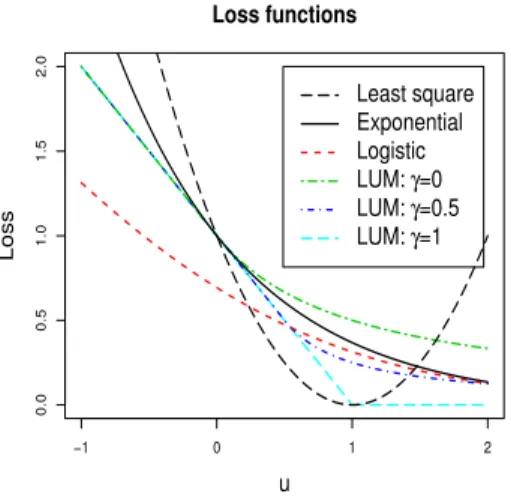
This section illustrates our classifier selection algorithm using the LUM [43] as an example. The LUM offers a platform unifying various large margin classifiers ranging from soft ones to hard ones. A soft classifier estimates the class conditional probabil-ities explicitly and makes the class prediction via the largest estimated probability, while a hard classifier directly estimates the classification boundary without a class-probability estimation [44]. For simplicity of presentation, we rewrite the class of LUM loss functions as
Lγ(u) = 1−u if u < γ (1−γ)2( 1 u−2γ+1) if u≥γ, (2.12)
where the index parameter γ ∈ [0,1]. As shown by [43], when γ = 1 the LUM loss reduces to the hinge loss of SVM, which is a typical example of hard classification; whenγ = 0.5 the LUM loss is equivalent to the DWD classifier, which can be viewed as a classifier that is between hard and soft; and whenγ = 0 the LUM loss becomes a
soft classifier that has an interesting connection with the logistic loss. Therefore, the LUM framework approximates many of the soft and hard classifiers in the literature. Figure 2.3 displays LUM loss functions for various values of γ and compares them with some commonly used loss functions.
Least square Exponential Logistic LUM: γ=0 LUM: γ=0.5 LUM: γ=1 −1 0 1 2 0.0 0.5 1.0 1.5 2.0 Loss functions u Loss
Figure 2.2. Plots of least square, exponential, logistic, and LUM loss functions withγ = 0,0.5,1.
In the LUM framework, we denote the true risk as Rγ(θ) = E[Lγ(yf(x;θ))], the
true parameter asθ0γ = arg minθRγ(θ), the GE asD0γ, the empirical generalization
error asDbγ, and the K-CV error as Dbγ. In practice, given dataDn, LUM solves
b θγ = arg min b,w ( 1 n n X i=1 Lγ yi(wTxi+b) +λnw Tw 2 ) . (2.13)
We next establish the asymptotic normality of Dbγ and θbγ (with more explicit
forms of the asymptotic variances) by verifying the conditions in Theorem 2.2.1, i.e., (L1)–(L5). In particular, we provide a set of sufficient conditions for the LUM, i.e., (L1) and (A1) below.
Assumption (A1) is needed to guarantee the uniqueness of the true minimizerθ0γ. It
is worth pointing out that the asymptotic normality of the estimated coefficients for SVM has also been established by Koo et al. (2008) under another set of assumptions.
Corollary 1 Suppose that Assumptions (L1) and (A1) hold and λn =o(n−1/2). We have, for each fixed γ ∈[0,1],
√
n(bθγ−θ0γ)
d
−→N(0,Σ0γ) as n → ∞, (2.14) where Σ0γ =H(θ0γ)−1G(θ0γ)H(θ0γ)−1 with G(θ0γ) andH(θ0γ)defined in (2.31) and (2.33) in Section 2.7.5.
In practice, direct estimation of Σ0γin (2.14) is difficult because of the involvement
of the Dirac delta function; see Section 2.7.5 for details. Instead, we find that the perturbation-based resampling procedure proposed in Stage 1 works well.
Next we establish the asymptotic normality of Dbγ.
Corollary 2 Suppose that the assumptions in Corollary 1 hold. We have, asn → ∞, √ n(Dbγ−D0γ) d −→N0, E(ψ21γ), (2.15) where ψ1γ = 12|Y1 −sign{f(X1;θ0γ)}| − D0γ − d˙(θ0γ)TH(θ0γ)−1M1(θ0γ), d˙(θ) = OθE(Dbγ(θ)), and M1(θ0γ) =−Y1X˜1I{Y1f(X1;θ0γ)<γ}− (1−γ)2Y1X˜1I{Y1f(X1;θ0γ)≥γ} Y1f(X1;θ0γ)−2γ+ 1 2 .
Corollary 2 demonstrates that the K-CV error induced from each LUM loss func-tion yields the desirable asymptotic property under Assumpfunc-tions (L1) and (A1). It can be applied to justify the perturbation-based resampling procedure for LUM as shown in Theorem 2.2.2.
2.4 Selection Consistency
This section investigates the selection consistency of our two-stage classifier se-lection algorithm. Sese-lection consistency means that the selected classifier achieves
the minimal GE and minimal DBI asymptotically. We focus on the selection consis-tency of the LUM loss functions in this section; the extension to other large-margin classifiers is straightforward.
For the LUM class, we define the set of potentially good classifiers as
b Λ0 = n γ ∈[0,1] :Dbγ ≤Db b γ∗ 0 +n −1/2φ γ,bγ ∗ 0;α/2 o , (2.16)
where bγ0∗ = arg minγ∈[0,1]Dbγ, based on Dn. Its population version is thus defined as
those classifiers achieving the minimal GE, denoted Λ0 =
n
γ ∈[0,1] :D0γ =D0γ0∗
o
, (2.17)
where γ0∗ = arg minγ∈[0,1]D0γ. Literally, bγ
∗
0 and γ
∗
0 may not be unique. To show
the selection consistency, we require an additional assumption on the Hessian matrix defined in Corollary 1:
(B1) The smallest eigenvalue of the true Hessian matrix λmin(H(θ0γ))≥c1, and the
largest eigenvalue of the true Hessian matrix λmax(H(θ0γ)) ≤ c2, where the
positive constants c1, c2 do not depend on γ.
As seen in the proof of Corollary 1, the true Hessian matrix H(θ0γ) is positive
definite for any fixed γ ∈ [0,1] under Assumptions (L1) and (A1). Therefore, As-sumption (B1) is slightly stronger in the uniform sense. It is required to guarantee the uniform convergence results, i.e., (2.38) and (2.40), in Appendix A.1.
Our Lemma 1 first ensures that the minimum K-CV error converges to the mini-mum GE at a root-n rate.
Lemma 1 Suppose that Assumptions (L1),(A1), and (B1) hold. We have, if λn =
o(n−1/2), Dbbγ ∗ 0 −D0γ ∗ 0 =OP(n −1/2). (2.18)
In the second stage, we denote the index of the selected optimal classifier as
b γ0 = arg min γ∈Λb0 [ DBIS(X;bθγ) , (2.19)
and its population version as γ0 = arg min γ∈Λ0 DBI S(X;bθγ) . (2.20)
Again, bγ0 and γ0 are not necessarily unique.
Theorem 2.4.1 Suppose the assumptions in Lemma 1 hold, we have, as N → ∞,
DBI[ S(X;bθ b γ0) −DBIS(X;bθγ0) =oP(n −1). (2.21)
Recall that N is the number of resamplings defined in Step 2 of Algorithm 1.
Theorem 2.4.1 implies that the estimated DBI of the selected classifier converges to the DBI of the true optimal classifier, which has the smallest DBI. Therefore, the proposed two-stage algorithm is able to select the classifier with the minimal DBI among those classifiers having the minimal GE. It is not uncommon to have several classifiers obtain the same minimal GE, especially when the two classes are well separable. In summary, we have shown that the selected optimal classifier has achieved the minimal GE and the minimal DBI asymptotically.
2.5 Experiments
In this section, we first demonstrate the DBI estimation procedure introduced in Section 2.2.2, and then illustrate the applicability of our classifier selection method in various simulated and real examples. In all experiments, we compare our selection procedure, denoted as “cv+dbi”, with two alternative methods: 1) “cv+varcv” which is the two-stage approach selecting the loss with the minimal variance of the K-CV error in Stage 2, and 2) “cv+be” which is the two-stage approach selecting the loss with the minimal classification stability defined in Bousquet and Elisseeff (2002) in Stage 2. Stage 1 of each alternative approach is the same as ours. We consider six large-margin classifier candidates: least squares loss, exponential loss, logistic loss, and LUM with γ = 0,0.5,1. Recall that LUM with γ = 0.5 (γ = 1) is equivalent to DWD (SVM). In all the large-margin classifiers, the tuning parameter λn is selected
2.5.1 Illustration
This subsection demonstrates the DBI estimation procedure and checks the sen-sitivity of the confidence level α in Algorithm 2.
We generated labelsy∈ {−1,1}with equal probability. GivenY =y, the predic-tor vecpredic-tor (x1, x2) was generated from a bivariate normal N((µy, µy)T, I2) with the
signal level µ= 0.8.
We first illustrate the DBI estimation procedure in Section 2.2.2 by comparing the estimated DBIs with the true DBIs for various sample sizes. We varied the sample size n among 50, 100, 200, 500, and 1000. The classifier with the least squares loss was investigated due to its simplicity. Simple algebra implied that the true parameter θ0L = (0,0.351,0.351) and the transformed parameter θ
†
0L= (0,0,0.429).
Furthermore, the covariance matrix Σ0L and the transformed covariance matrix Σ † 0L were computed as Σ0L= 0.439 0 0 0 0.268 −0.170 0 −0.170 0.268 and Σ†0L = 0.439 0 0 0 0.439 0 0 0 0.098 ,
given the transformation matrix
RL= − √ 2 2 √ 2 2 √ 2 2 √ 2 2 .
Finally, plugging all these terms into (2.8) led to
DBIS(X;bθL)
≈ 3.563
n . (2.22)
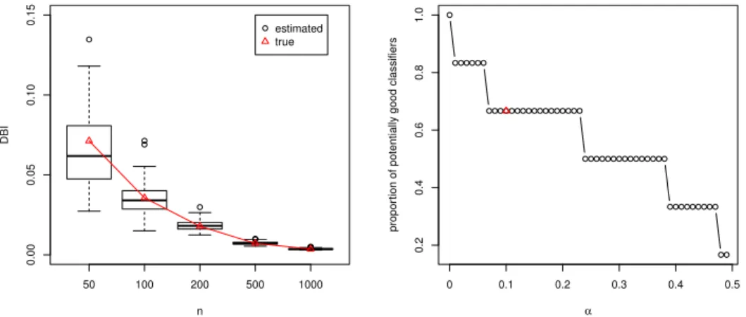
The left plot of Figure 2.5.1 compares the estimated DBIs in (2.10) with the true DBIs in (2.22). Clearly, they match very well for various sample sizes and their difference vanishes as the sample size increases. This experiment empirically validates the estimation procedure in Section 2.2.2.
In order to show the sensitivity of the confidence levelαto the set Λ in Algorithm 2, we randomly selected one replication and display the proportion of potentially good
n DBI 50 100 200 500 1000 0.00 0.05 0.10 0.15 estimated true 0 0.1 0.2 0.3 0.4 0.5 0.2 0.4 0.6 0.8 1.0 α propor
tion of potentially good classifiers
Figure 2.3. Comparison of true and estimated DBIs in Example 6.1 is shown in the left plot. The true DBIs are denoted as red triangles and the estimated DBIs from replicated experiments are illustrated by box plots. The sensitivity of confidence level α to the proportion of potentially good classifiers in Stage 1 is shown on the right.
classifiers over all six classifiers. Note that as α increases, the confidence interval for the difference of GEs will be narrower, and hence the size of Λ will be smaller. Therefore, the change of the proportion reflects exactly the change of Λ since Λ is monotone with respect to α. For each α ∈ { l
100; l = 0, . . . ,50}, we computed the
proportion of potentially good classifiers. As shown in the right plot of Figure 2.5.1, the proportion is stable in a reasonable range around 0.1.
2.5.2 Simulations
In this section, we illustrate the superior performance of our method using four simulated examples. These simulations were previously studied by [45] and [43]. In all of the simulations, the size of training data sets was 100 and that of testing data sets was 1000. All the procedures were repeated 100 times and the averaged test errors and averaged test DBIs of the selected classifier were reported.
Simulation 1: Two predictors were uniformly generated over{(x1, x2) :x21+x22 ≤
1}. The class label y was 1 when x2 ≥ 0 and −1 otherwise. We generated 100
samples and then contaminated the data by randomly flipping the labels of 15% of the instances.
Simulation 2: The setting was the same as Simulation 1 except that we contam-inated the data by randomly flipping the labels of 25% of the instances.
Simulation 3: The setting was the same as Simulation 1 except that we con-taminated the data by randomly flipping the labels of 80% of the instances whose |x2| ≥0.7.
Simulation 4: Two predictors were uniformly generated over {(x1, x2) : |x1|+
|x2| ≤ 2}. Conditionally on X1 = x1 and X2 = x2, the class label y took 1 with
probability e3(x1+x2)/(1 +e3(x1+x2)) and −1 otherwise.
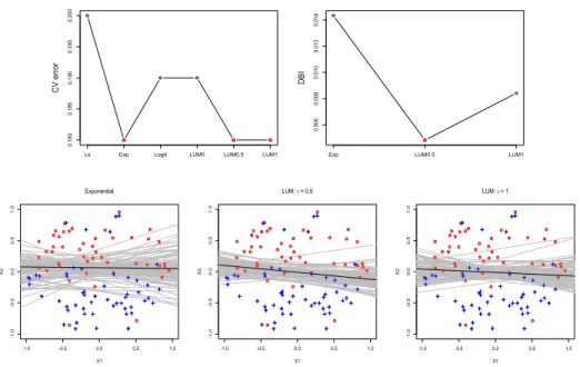
We first demonstrate the mechanism of our proposed method for one repetition of Simulation 1. As shown in the upper left plot of Figure 2.5.2, exponential loss and LUMs with γ = 0.5 or 1 are potentially good classifiers in Stage 1; they happen to have the same K-CV error. Their corresponding DBIs are compared in the second stage. As shown in the upper right plot of Figure 2.5.2, LUM with γ = 0.5 gives the minimal DBI and is selected as the final classifier. In this example, although exponential loss also gives the minimal K-CV error, its decision boundary is unstable compared to that of LUM with γ = 0.5. This shows that the K-CV estimate itself is not sufficient for classifier comparison, since it ignores the variation in the classifier. To show that our DBI estimation is reasonable, we display the perturbed decision boundaries for these three potentially good classifiers on the bottom of Figure 2.5.2. The relationship among their instabilities is precisely captured by our DBI estimate: compared with the exponential loss and LUM with γ = 1, LUM withγ = 0.5 is more stable.
We report the averaged test errors and averaged test DBIs of the classifier selected from our method as well as two alternative approaches, see Table 2.1. In all four sim-ulated examples, our “cv+dbi” achieves the smallest test errors, while the difference
Ls Exp Logit LUM0 LUM0.5 LUM1 0.180 0.185 0.190 0.195 0.200 C V erro r
Exp LUM0.5 LUM1
0.006 0.008 0.010 0.012 0.014 D BI -1.0 -0.5 0.0 0.5 1.0 -1 .0 -0 .5 0.0 0.5 1.0 Exponential X1 X2 -1.0 -0.5 0.0 0.5 1.0 -1 .0 -0 .5 0.0 0.5 1.0 LUM: γ = 0.5 X1 X2 -1.0 -0.5 0.0 0.5 1.0 -1 .0 -0 .5 0.0 0.5 1.0 LUM: γ = 1 X1 X2
Figure 2.4. The K-CV error, the DBI estimate, and the perturbed decision boundaries in Simulation 1 with flipping rate 15%. The min-imal K-CV error and minmin-imal DBI estimate are indicated with red triangles. The labels Ls, Exp, Logit, LUM0, LUM0.5, and LUM1 re-fer to least squares loss, exponential loss, logistic loss, and LUM loss with index γ = 0,0.5,1, respectively.
among test errors of all algorithms is generally not significant. This phenomenon of indistinguishable test errors agrees with the fact that all methods are the same during the first stage and those left from Stage 1 are all potentially good in terms of classification accuracy. However, our “cv+dbi” is able to choose the classifiers with minimal test DBIs in all simulations and the improvements over other algorithms are significant. Overall, our method is able to choose the classifier with outstanding performance in both classification accuracy and stability.
2.5.3 Real Examples
In this subsection, we compare our method with the alternatives on two real datasets in the UCI Machine Learning Repository [46].
Table 2.1.
The averaged test errors and averaged test DBIs (multiplied by 100) of all methods: “cv+varcv” is the two-stage approach which selects the loss with the minimal variance of the K-CV error in Stage 2; “cv+be” is the two-stage approach which in Stage 2 selects the loss with the minimal classification stability defined in Bousquet and Elis-seeff (2002); “cv+dbi” is our method. The smallest value in each case is given in bold. Standard errors are given in subscript.
Simulations cv+varcv cv+be cv+dbi
Sim 1 Error 0.1910.002 0.1940.002 0.1900.002 DBI 0.1390.043 0.1350.019 0.0810.002 Sim 2 Error 0.2960.002 0.3030.003 0.2950.002 DBI 0.2910.044 0.3180.036 0.2290.012 Sim 3 Error 0.2180.006 0.2340.006 0.2090.004 DBI 0.1240.008 0.2910.037 0.1070.003 Sim 4 Error 0.1200.001 0.1210.001 0.1190.001 DBI 0.8840.207 0.4140.106 0.2350.038
The first data set is the liver disorders data set (liver) which consists of 345 samples with 6 variables of blood test measurements. The class label splits the data into 2 classes with sizes 145 and 200. The second data set is the breast cancer data set (breast) which consists of 683 samples after removing missing values [47]. Each sample has 10 experimental measurement variables and one binary class label indicating whether the sample is benign or malignant. These 683 samples arrived periodically as Dr. Wolberg reported his clinical cases. In total, there are 8 groups of samples which reflect the chronological order of the data. It is expected that a good classification procedure should generate a classifier that is stable across these groups of samples.
For each dataset, we randomly split the data into 2/3 training samples and 1/3 testing samples, and reported the averaged test errors and averaged test DBIs based
on all classifier selection algorithms over 50 replications, see Table 2.2. Compared with the alternatives, our “cv+dbi” method obtains significant improvements in DBIs and simultaneously attains minimal test errors in both real data sets. This indicates that the proposed method could serve as a practical tool for selecting a most accurate and stable classifier.
Table 2.2.
The averaged test errors and averaged test DBIs of all methods in real example. The smallest value in each case is given in bold. Standard errors are given in subscript.
Data cv+varcv cv+be cv+dbi
Liver Error 0.3310.006 0.3350.006 0.3270.006
DBI 0.1400.013 0.1570.024 0.1130.012
Breast Error 0.0380.002 0.0380.002 0.0380.002
DBI 0.3880.066 0.1520.028 0.1240.023
2.6 Nonlinear Extension
The extension of our two-stage algorithm to nonlinear classifiers contains two aspects: (1) asymptotic normality of the K-CV error in Stage 1; (2) the application of DBI in Stage 2. The former is still valid due to [48], and the latter is feasible by mapping the nonlinear decision boundaries to a higher dimensional space where the projected decision boundaries are linear. Details of these two extensions are as follows.
Extension of Stage 1: We first modify several key concepts. The loss L:X × Y ×R→[0,∞) is convex if it is convex in its third argument for every (x, y)∈ X × Y. A reproducing kernel Hilbert space (RKHS) H is a space of functionsf :X → Rwhich is generated by a kernel k : X × X →R. Here the kernel k could be a linear kernel, a Gaussian RBF kernel, or a polynomial kernel.
Given i.i.d training samples Dn ={(xi, yi);i= 1, . . . , n} drawn fromP = (X, Y),
the empirical function fL,Dn,λn solves
min f∈H 1 n n X i=1 L(xi, yi, f(xi)) +λnkfk2H.
In the nonparametric case, the optimization problem of minimizing population risk is ill-posed because a solution is not necessarily unique, and small changes in P
may have large effects on the solution. Therefore it is common to impose a bound on the complexity of the predictor and estimate a smoother approximation to the population version [48]. For a fixed λ0 ∈(0,∞), we denote fL,P,λ0 as the population
function which solves min
f∈H
Z
L(x, y, f(x))P(d(x, y)) +λ0kfk2H.
The following conditions are assumed in [48] to prove the asymptotic normality of the estimated kernel decision function.
(N1) The loss L is a convex, P-square-integrable Nemitski loss function of order
p∈[1,∞). That is, there is a P-square-integrable function b :X × Y → R such that |L(x, y, t)| ≤b(x, y) +|t|p for every (x, y, t)∈ X × Y ×
R.
(N2) The partial derivatives L0(x, y, t) := ∂L
∂t(x, y, t) and L 00
(x, y, t) := ∂2L
∂2t(x, y, t)
exist for every (x, y, t)∈ X × Y ×R and are continuous. (N3) For every a ∈ (0,∞), there is b0a ∈L2(P) and b
00
a ∈ [0,∞) such that, for every
(x, y)∈ X × Y, supt∈[−a,a]|L0(x, y, t)| ≤ba0(x, y) and supt∈[−a,a]|L00(x, y, t)| ≤b00a.
Proposition 1 (Theorem 3.1, [48]) Under Assumptions (N1)-(N3) and λn = λ0+
o(n−1/2), for every λ0 ∈ (0,∞), there is a tight, Borel-measurable Gaussian process
H: Ω→H such that
√
nfL,Dn,λn−fL,P,λ0
→H.
Remark 2 Among the loss functions considered in this paper, the least squares, ex-ponential, and logistic losses all satisfy the assumptions (N1)-(N3), while the LUM loss is not differentiable and does not satisfy Assumption (N2). However, [48] showed that any Lipschitz-continuous loss function (e.g. LUM loss) can always be modified as
a differentiable −version of the loss function such that the assumptions (N1)-(N3) are satisfied; see Remark 3.5 in [48].
In the nonlinear case, the GE D0L and the K-CV error DbL are modified
accord-ingly. The asymptotic normality of WL = √
n(DbL−D0L) follows from Proposition
1, Corollary 3.3 in [49], and a slight modification of the proof of our Theorem 1. Then a perturbation-based resampling approach can be constructed analogously to Algorithm 1.
Extension of Stage 2: The concept of DBI is defined for linear decision bound-aries. In order to measure the instability of nonlinear decision boundaries, we can map the nonlinear decision boundaries to a higher dimensional space where the projected decision boundaries are linear.
−2 0 2 4 −2 0 2 4 Least square X1 X2 −2 0 2 4 −2 0 2 4 SVM X1 X2
Figure 2.5. The nonlinear perturbed decision boundaries for the least squares loss (left) and SVM (right) in the bivariate normal example with unequal variances.
Here we illustrate the estimation procedure via a bivariate normal example with sample size n = 400. Assume the underlying distributions of the two classes are
f1 = N((−1,−1)T, I2) and f2 = N((1,1)T,2I2) with equal prior probability. We