Machine Learning Techniques in Spam Filtering
Konstantin Tretyakov, [email protected]
Institute of Computer Science, University of Tartu
Data Mining Problem-oriented Seminar, MTAT.03.177,
May 2004, pp. 60-79.
Abstract
The article gives an overview of some of the most popular machine learning methods (Bayesian classification, k-NN, ANNs, SVMs) and of their applicability to the problem of spam-filtering. Brief descriptions of the algorithms are presented, which are meant to be understandable by a reader not familiar with them before. A most trivial sample im-plementation of the named techniques was made by the author, and the comparison of their performance on the PU1 spam corpus is presented. Finally, some ideas are given of how to construct a practically useful spam filter using the discussed techniques. The article is related to the author’s first attempt of applying the machine-learning techniques in practice, and may therefore be of interest primarily to those getting aquainted with machine-learning.
1
Introduction
True loneliness is when you don’t even receive spam.
It is impossible to tell exactly who was the first one to come upon a simple idea that if you send out an advertisement to millions of people, then at least one person will react to it no matter what is the proposal. E-mail provides a perfect way to send these millions of advertisements at no cost for the sender, and this unfortunate fact is nowadays extensively exploited by several organizations. As a result, the e-mailboxes of millions of people get cluttered with all this so-called unsolicited bulk e-mail also known as “spam” or “junk mail”. Being increadibly cheap to send, spam causes a lot of trouble to the Internet community: large amounts of spam-traffic between servers cause delays in delivery of legitimate e-mail, people with dial-up Internet access have to spend bandwidth downloading junk mail. Sorting out the unwanted messages takes time and introduces a risk of deleting normal mail by mistake. Finally, there is quite an amount of pornographic spam that should not be exposed to children.
Many ways of fighting spam have been proposed. There are “social” methods like legal measures (one example is an anti-spam law introduced in the US [21]) and plain personal involvement (never respond to spam, never publish your e-mail address on webpages, never forward chain-letters. . . [22]). There are
“technological” ways like blocking spammer’s IP-address, and, at last, there is e-mail filtering. Unfortunately, no universal and perfect way for eliminating spam exists yet, so the amount of junk mail keeps increasing. For example, about 50% of the messages coming to my personal mailbox is spam.
Automatic e-mail filtering seems to be the most effective method for coun-tering spam at the moment and a tight competition between spammers and spam-filtering methods is going on: the finer the anti-spam methods get, so do the tricks of the spammers. Only several years ago most of the spam could be reliably dealt with by blocking e-mails coming from certain addresses or filtering out messages with certain subject lines. To overcome this spammers began to specify random sender addresses and to append random characters to the end of the message subject. Spam filtering rules adjusted to consider separate words in messages could deal with that, but then junk mail with specially spelled words (e.g. B-U-Y N-O-W) or simply with misspelled words (e.g. BUUY NOOW) was born. To fool the more advanced filters that rely on word frequencies spammers append a large amount of “usual words” to the end of a message. Besides, there are spams that contain no text at all (typical are HTML messages with a sin-gle image that is downloaded from the Internet when the message is opened), and there are even self-decrypting spams (e.g. an encrypted HTML message containing Javascript code that decrypts its contents when opened). So, as you see, it’s a never-ending battle.
There are two general approaches to mail filtering: knowledge engineering (KE) and machine learning (ML). In the former case, a set of rules is created according to which messages are categorized as spam or legitimate mail. A typical rule of this kind could look like “if the Subject of a message contains the text BUY NOW, then the message is spam”. A set of such rules should be created either by the user of the filter, or by some other authority (e.g. the software company that provides a particular rule-based spam-filtering tool). The major drawback of this method is that the set of rules must be constantly updated, and maintaining it is not convenient for most users. The rules could, of course, be updated in a centralized manner by the maintainer of the spam-filtering tool, and there is even a peer-2-peer knowledgebase solution1, but when
the rules are publicly available, the spammer has the ability to adjust the text of his message so that it would pass through the filter. Therefore it is better when spam filtering is customized on a per-user basis.
The machine learning approach does not require specifying any rules explic-itly. Instead, a set of pre-classified documents (training samples) is needed. A specific algorithm is then used to “learn” the classification rules from this data. The subject of machine learning has been widely studied and there are lots of algorithms suitable for this task.
This article considers some of the most popular machine learning algo-rithms and their application to the problem of spam filtering. More-or-less self-contained descriptions of the algorithms are presented and a simple com-parison of the performance of my implementations of the algorithms is given. Finally, some ideas of improving the algorithms are shown.
2
Statement of the Problem
Email is not just text; it has structure. Spam filtering is not just classification, because false positives are so much worse than false negatives that you should treat them as a different kind of error. And the source of error is not just random variation, but a live human spammer working actively to defeat your filter.
P. Graham. Better Bayesian Filtering.
What we ultimately wish to obtain is a spam filter, that is: a decision function f, that would tell us whether a given e-mail message m is spam (S) or legitimate mail (L). If we denote the set of all e-mail messages by M, we
may state that we search for a function f : M → {S, L}. We shall look for
this function by training one of the machine learning algorithms on a set of pre-classified messages {(m1, c1),(m2, c2), . . . ,(mn, cn)},mi ∈M, ci ∈ {S, L}. This is nearly a general statement of the standard machine learning problem. There are, however, two special aspects in our case: we have to extract features from text strings and we have some very strict requirements for the precision of our classifier.
2.1
Extracting Features
The objects we are trying to classify are text messages, i.e. strings. Strings are, unfortunately, not very convenient objects to handle. Most of the machine learning algorithms can only classify numerical objects (real numbers or vectors) or otherwise require some measure of similarity between the objects (a distance metric or scalar product).
In the first case we have to convert all messages to vectors of numbers(feature vectors) and then classify these vectors. For example, it is very customary to take the vector of numbers of occurences of certain words in a message as the feature vector. When we extract features we usuallylose information and it is clear that the way we define our feature-extractor is crucial for the performance of the filter. If the features are chosen so that there may exist a spam message and a legitimate mail with the same feature vector, then no matter how good our machine learning algorithm is, it will make mistakes. On the other hand, a wise choice of features will make classification much easier (for example, if we could choose to use the “ultimate feature” of being spam or not, classification would become trivial). It is worth noting, that the features we extract need not all be taken only from the message text and we may actually add information in the feature extraction process. For example, analyzing the availability of the internet hosts mentioned in theReturn-PathandReceivedmessage headers may provide some useful information. But once again, it is much more important what features we choose for classification than what classification algorithm we use. Oddly enough, the question of how to choose “really good” features seems to have had less attention, and I couldn’t find many papers on this topic [1]. Most of the time the basic vector of word frequencies or something similar is used. In this article we shall not focus on feature extraction either. In the following we shall denote feature vectors with letter x and we use m for messages.
Now let us consider those machine learning algorithms that require distance metric or scalar product to be defined on the set of messages. There does exist a suitable metric (edit distance), and there is a nice scalar product defined purely for strings (see [2]), but the complexity of the calculation of these functions is a bit too restrictive to use them in practice. So in this work we shall simply extract the feature vectors and use the distance/scalar product of these vectors. As we are not going to use sophisticated feature extractors, this is admittedly a major flaw in the approach.
2.2
Classifier Performance
Our second major problem is that the performance requirements of a spam filter are different from those of a “usual” classifier. Namely, if a filter misclassifies junk message as a legitimate one, it is a rather light problem that does not cause too much trouble for the user. Errors of the other kind—mistakingly classifying legitimate mail as spam—are, however, completely unacceptable. Really, there is no much sense in a spam filter, that sometimes filters legitimate mail as spam, because in this case the user has to review the messages sorted out to the “spam folder” regularly, and that somehow defeats the whole purpose of spam filtering. A filter that makes such misclassifications very rarely is not much better because then the user tends to trust the filter, and most probably does not review the messages that were filtered out, so if the filter makes a mistake, an important email may get lost. Unfortunately, in most cases it is impossible to reliably ensure that a filter will not have these so-calledfalse positives. In most of the learning algorithms there is a parameter that we may tune to increase the importance of classifying legitimate mail correctly, but we can’t be too liberal with it, because if we assign too high importance to legitimate mail, the algorithm will simply tend to classify all messages as non-spam, thus making indeed no dangerous decisions, but having no practical value [6].
Some safety measures may compensate for filter mistakes. For example, if a message is classified as spam, a reply may be sent to the sender of that message prompting to resend his message to another address or to include some specific words in the subject [6].2 Another idea is to use a filter to estimate the certainty that given message is spam and sort the list of messages in the user’s mailbox in ascending order of this certainty [11].
3
The Algorithms: Theory
This section gives a brief overview of the underlying theory and implementations of the algorithms we consider. We shall discuss thena¨ıve Bayesian classifier, the k-NN classifier, the neural network classifier and the support vector machine classifier.
2Note that this is not an ultimate solution. For example, messages from mailing-lists may
3.1
The Na¨ıve Bayesian Classifier
3.1.1 Bayesian ClassificationSuppose that we knew exactly, that the wordBUYcould never occur in a legiti-mate message. Then when we saw a message containing this word, we could tell for sure that it were spam. This simple idea can be generalized using some prob-ability theory. We have two categories (classes): S (spam) and L (legitimate mail), and there is a probability distribution of messages (or, more precisely, the feature vectors we assign to messages) corresponding to each class: P(x|c) denotes the probability3of obtaining a message with feature vectorxfrom class
c. Usually we know something about these distributions (as in example above, we knew that the probability of receiving a message containing the word BUY
from the category L was zero). What we want to know is, given a message
x, what category c “produced” it. That is, we want to know the probability P(c|x). And this is exactly what we get if we use theBayes’ rule:
P(c|x) =P(x|c)P(c) P(x) =
P(x|c)P(c)
P(x|S)P(S) +P(x|L)P(L)
where P(x) denotes the a-priori probability of messagex and P(c) — the a-priori probability of classc(i.e. the probability that a random message is from that class). So if we know the values P(c) and P(x|c) (for C ∈ {S, L}), we may determine P(c|x), which is already a nice achievement that allows us to use the following classification rule:
IfP(S|x)> P(L|x) (that is, if thea-posteriori probability thatxis spam is greater than the a-posteriory probability thatxis non-spam), classifyx
as spam, otherwise classify it as legitimate mail.
This is the so-calledmaximum a-posteriori probability (MAP) rule. Using the Bayes’ formula we can transform it to the form:
If PP((xx||LS))> PP((LS))classifyxas spam, otherwise classify it as legitimate mail. It is common to denote thelikelihood ratio PP((xx||SL)) as Λ(x) and write the MAP rule in a compact way:
Λ(x) S ≷ L P(L) P(S)
But let us generalize a bit more. Namely, letL(c1, c2) denote thecost (loss, risk) of misclassifying an instance of classc1 as belonging to classc2 (and it is natural to have L(S, S) = L(L, L) = 0 but in a more general setting this may not always be the case). Then, theexpected risk of classifying a given message
xto class cwill be:
R(c|x) =L(S, c)P(S|x) +L(L, c)P(L|x)
It is clear that we wish our classifier to have small expected risk for any message, so it is natural to use the following classification rule:
3To be more formal we should have written something likeP(X =x|C=c). We shall,
IfR(S|x)< R(L|x) classifyxas spam, otherwise classify it as legitimate mail.4
This rule is called the Bayes’ classification rule (or Bayesian classifier). It is easy to show that Bayesian classifier (denote it by f) minimises the overall expected risk5 (average risk) of the classifier
R(f) = Z L(c, f(x)) dP(c,x) =P(S) Z L(S, f(x)) dP(x|S) +P(L) Z L(L, f(x)) dP(x|L) and thereforeBayesian classifier is optimal in this sense [14].
In spam categorization it is natural to setL(S, S) =L(L, L) = 0. We may then rewrite the final classification rule in the form of a likelihood ratio:
Λ(x) S ≷ L λP(L) P(S)
where λ = LL((L,SS,L)) is the parameter that specifies how “dangerous” it is to misclassify legitimate mail as spam. The greater is λ, the less false positives will the classifier produce.
3.1.2 The Na¨ıve Bayesian Classifier
Now that we have discussed the beautiful theory of the optimal classifier, let us consider the not-so-simple practical application of the idea. In order to construct Bayesian classifier for spam detection we must somehow be able to determine the probabilities P(x|c) andP(c) for any x and c. It is clear that we can never know them exactly, but we may estimate them from the training data. For example, P(S) may be approximated by the ratio of the number of spam messages to the number of all messages in the training data. Estimation of P(x|c) is much more complex and actually depends on how we choose the feature vector x for message m. Let us try the most simple case of a feature vector with a single binary attribute that denotes the presence of a certain word win the message. That is, we define the message’s feature vectorxwto be, say, 1 if the word w is present in the message, and 0 otherwise. In this case it is simple to estimate the required probabilities from data: for example
P(xw= 1|S)≈
number of training spam messages containing the wordw total number of training spam messages
So if we fix a word w we have everything we need to calculate Λ(xw) and so we may use the Bayesian classifier described above. Here is the summary of the algorithm that results:
• Training
1. Calculate estimates for P(c), P(xw = 1|c), P(xw = 0|c) (for c = S, L) from the training data.
4Note that in the case whenL(S, L) =L(L, S) = 1 andL(S, S) =L(L, L) = 0 we have
R(S|x) =P(L|x) andR(L|x) =P(S|x) so this rule reduces to the MAP rule.
5The proof follows straight from the observation thatR(f) =R
2. CalculateP(c|xw= 0),P(c|xw= 1) using the Bayes’ rule. 3. Calculate Λ(xw) forxw= 0,1, calculateλ
P(L)
P(S). Store these 3 values.
6
• Classification
1. Given a messagemdeterminexw, retrieve the stored value for Λ(xw) and use the decision rule to determine the category of messagem. Now this classifier will hardly be any good because it bases its decisions on the presence or absence of one word in a message. We could improve the situation if our feature vector contained more attrubutes. Let us fix several words w1, w2, . . . , wm and define for a message m its feature vector as x = (x1, x2, . . . , xm) wherexiis equal to 1 if the wordwiis present in the message, and 0 otherwise. If we followed the algorithm described above, we would have to calculate and store the values of Λ(x) for all possible values ofx(and there are 2mof them). This is not feasible in practice, so we introduce an additional assumption: we assume that the components of the vectorxareindependent in each class. In other words, the presence of one of the wordswiin a message does not influence the probability of presence of other words. This is a very wrong assumption, but it allows us to calculate the required probabilities without having to store large amounts of data, because due to independence
P(x|c) = m Y i=1 P(xi|c) Λ(x) = m Y i=1 Λi(xi)
So the algorithm presented above is easily adapted to become theNa¨ıve Bayesian classifier. The word “na¨ıve” in the name expresses the na¨ıveness of the assump-tion used. Interestingly enough, the algorithm performs rather well in practice, and currently it is one of the most popular solutions used in spam filters.7 Here
it is:
• Training
1. For all wi calculate and store Λi(xi) for xi = 0,1. Calculate and storeλPP((LS)).
• Classification
1. Determine x, calculate Λ(x) by multiplying the stored values for Λi(xi). Use the decision rule.
The remaining question is which words to choose for determining the at-tributes of the feature vector. The most simple solution is to use all the words present in the training messages. If the number of words is too large it may be reduced using different techniques. The most common way is to leave out words
6Of course it would be enough to store only two bits: the decision for the casex
w= 0 and
for the casexw= 1, but we’ll need the Λ in the following, so let us keep it.
7It is worth noting, that there were successful attempts to use some less “na¨ıve”
that are too rare or too common. It is also common to select the most relevant words using the measure of mutual information [10]:
M I(Xi, C) = X xi=0,1 X c=S,L P(xi, c) log P(xi, c) P(xi)P(c)
We won’t touch this subject here, however, and in our experiment we shall simply use all the words.
3.2
k
Nearest Neighbors Classifier
Suppose that we have some notion of distance between messages. That is, we are able to tell for any two messages how “close” they are to each other. As already noted before, we may often use the eucledian distance between the feature vectors of the messages for that purpose. Then we may try to classify a message according to the classes of its nearest neighbors in the training set. This is the idea of thek nearest neigbor algorithm:
• Training
1. Store the training messages.
• Classification
1. Given a message x, determine its k nearest neighbors among the messages in the training set. If there are more spams among these neighbors, classify given message as spam. Otherwise classify it as legitimate mail.
As you see there is practically no “training” phase in its usual sense. The cost of that is the slow decision procedure: in order to classify one document we have to calculate distances to all training messages and find the k nearest neighbors. This (in the most trivial implementation) may take about O(nm) time for a training set ofnmessages containing feature vectors withmelements. Performing some clever indexing in the training phase will allow to reduce the complexity of classifying a message to about O(n) [1]. Another problem of the presented algorithm is that there seems to be no parameter that we could tune to reduce the number of false positives. This problem is easily solved by changing the classification rule to the followingl/k-rule:
Iflor more messages among theknearest neighbors ofxare spam, classify
xas spam, otherwise classify it as legitimate mail.
The k nearest neighbor rule has found wide use in general classification tasks. It is also one of the few universally consistent classification rules. We shall explain that now.
Suppose we have chosen a setsn of ntraining samples. Let us denote the k-NN classifier corresponding to that set as fsn. As described in the previous
section, it is possible to determine certain average riscR(fsn) of this classifier.
We shall denote it byRn. Note thatRn depends on the choice of the training set and is therefore a random variable. We know that this risk is always greater than the riskR∗ of the Bayesian classifier. However, we may hope that if the
size of the training set is large enough, the risk of the resultingk-NN classifier will be close to the optimal riskR∗. That property is calledconsistency.
Definition A classification rule is called consistent, if the expectation of the average risk E(Rn) converges to the optimal (Bayesian) risk R∗ as n goes to
infinity:
E(Rn) n
→R∗
We call a rulestrongly consistent if Rn
n
→R∗ almost everywhere
If a rule is (strongly) consistent for any distribution of (x, c), the rule is called universally (strongly) consistent.
Therefore consistency is a very good feature because it allows to increase the quality of classification by adding training samples. Universal consistency means that this holds for any distribution of training samples and their cate-gories (in particular: independently of whose mail messages are being filtered and what kind of messages is understood under “spam”). And, as already men-tioned before, thek-NN rule is (under certain conditions) universally consistent. Namely, the following theorem holds:
Theorem (Stone, 1977)Ifk→ ∞and nk →0, thenk-NN rule is universally consistent.
It is also possible to show, that if the distribution of training samples is continuous (i.e. it owns a probability density function), then k-NN rule is uni-versally strongly consistent under the conditions of the previous theorem [14].
Unfortunately, despite all these beautiful theoretical results, it occured to be very difficult to make thek-NN algorithm show good results in practice.
3.3
Artificial Neural Networks
Artificial neural networks (ANN-s) is a large class of algorithms applicable to classification, regression and density estimation. In general, a neural network is a certain complex function that may be decomposed into smaller parts(neurons, processing units) and represented graphically as a network of these neurons. Quite a lot of functions may be represented this way, and therefore it is not always clear which algorithms belong to the field of neural networks, and which do not. There are, however the two “classical” kinds of neural networks, that are most often meant when the term ANN is used: the perceptron and the multilayer perceptron. We shall focus on the perceptron algorithm, and provide some thoughts on the applicability of the multilayer perceptron.
3.3.1 The Perceptron
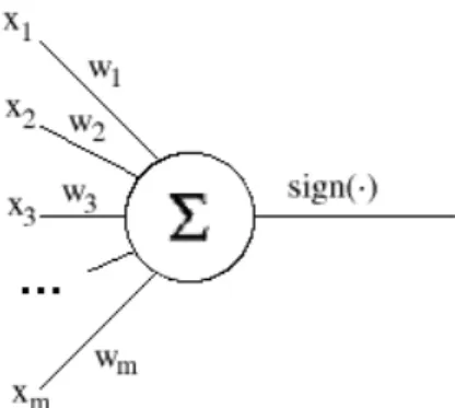
The idea of the perceptron is to find a linear function of the feature vector f(x) =wTx+b such thatf(x)>0 for vectors of one class, andf(x)<0 for vectors of other class. Here w = (w1, w2, . . . , wm) is the vector of coefficients (weights) of the function, and b is the so-called bias. If we denote the classes by numbers +1 and −1, we can state that we search for a decision function d(x) = sign(wTx+b). The decision function can be represented graphically as a “neuron”, and that is why the perceptron is considered to be a “neural
Figure 1: Perceptron as a neuron
network”. It is the most trivial network, of course, with a single processing unit.
If the vectors to be classified have only two components (i.e. x∈R2), they
can be represented as points on a plane. The decision function of a perceptron can then be represented as a line that divides the plane in two parts. Vectors in one half-plane will be classified as belonging to one class, vectors in the other half-plane—as belonging to the other class. If the vectors have 3 components, the decision boundary will be a plane in the 3-dimensional space, and in general, if the space of feature vectors isn-dimensional, the decision boundary is an n-dimensional hyperplane. This is an illustration of the fact that the perceptron is alinear classifier.
The perceptron learning is done with an iterative algorithm. It starts with arbitrarily chosen parameters (w0, b0) of the decision function and updates them iteratively. On the n-th iteration of the algorithm a training sample (x, c) is chosen such that the current decision function does not classify it correctly (i.e. sign(wT
nx+bn)6=c). The parameters (wn, bn) are then updated using the rule: wn+1=wn+cx bn+1=bn+c
The algorithm stops when a decision function is found that correctly classifies all the training samples. If such a function does not exist (i.e. the classes are notlinearly separable), the learning algorithm will never converge, and the perceptron is not applicable in this case. The fact that in case of linearly separable classes the perceptron algorithm converges is known as thePerceptron Convergence Theorem and was proven by Frank Rosenblatt in 1962. The proof is available in any relevant textbook [2,3,4].
When data is not linearly separable the best we can do is stop the training algorithm when the number of misclassifications becomes small enough. In our experiments, however, the data was always linearly separable.8
To conclude, here’s the summary of the perceptron algorithm:
8This is not very surprising, because the size of feature vectors we used was much greater
• Training
1. Initializew andb(to random values or to 0).
2. Find a training example (x, c) for which sign(wTx+b)6=c. If there is no such example, training is completed. Store the final w and b and stop. Otherwise go to next step.
3. Update (w, b): w:=w+cx,b:=b+c. Go to previous step.
• Classification
1. Given a message x, determine its class as sign(wTx+b). 3.3.2 Multilayer Perceptron
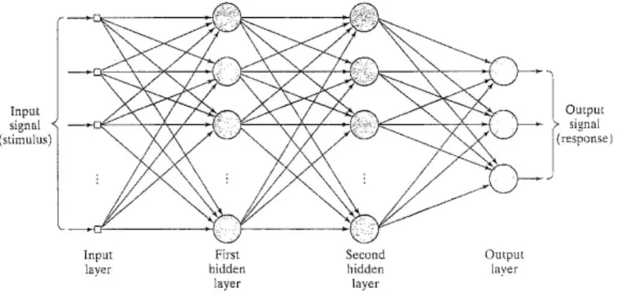
Multilayer perceptron is a function that may be visualized as a network with several layers of neurons, connected in a feedforward manner. The neurons in the first layer are calledinput neurons, and represent input variables. The neu-rons in the last layer are calledoutput neuronsand provide function result value. The layers between the first and the last are calledhidden layers. Each neuron in the network is similar to a perceptron: it takes input valuesx1, x2, . . . xk, and calculates its output valueoby the formula
o=φ( k X
i=1
wixi+b)
where wi, b are the weights and the bias of the neuron and φ is a certain nonlinear function. Most oftenφ(x) is is either 1+1eax or tanh(x).
Figure 2: Structure of a multilayer perceptron
Training of the multilayer perceptron means searching for such weights and biases of all the neurons for which the network will have as small error on the training set as possible. That is, if we denote the function implemented by in general position are linearly separable in any way (being in general position means that no kof the points lie in ak−2-dimensional affine subspace). The fact that feature space dimension is larger than the number of training samples may mean that we have “too many features” and this is not always good (see [11])
the network as f(x), then in order to train the network we have to find the parameters that minimize the total training error:
E(f) = n X
i=1
|f(xi)−ci|2
where (xi, ci) are training samples. This minimization may be done by any iterative optimization algorithm. The most popular is simple gradient descent, which in this particular case bears the name of error backpropagation. The detailed specification of this algorithm is presented in many textbooks or papers (see [3,4, 16]).
Multilayer perceptron is a nonlinear classifier: it models a nonlinear decision boundary between classes. As it was mentioned in the previous section, the training data that we used here was linearly separable, and using a nonlinear decision boundary could hardly improve generalization performance. Therefore the best result we could expect is the result of the simple perceptron. Another problem in our case is that implementation of efficient backpropagation learning for a network with about 20000 input neurons is quite nontrivial. So the only feasible way of applying multilayer perceptron would be to reduce the number of features to a reasonable amount. This paper does not deal with feature selection and therefore won’t deal with practical application of the multilayer perceptron either.
It should be noted, that of all the machine learning algorithms, the multilayer perceptron has, perhaps, the largest number of parameters that must be tuned in an ad-hoc manner. It is not very clear how many hidden neurons should it contain, and what parameters for the backpropagation algorithm should be chosen in order to achieve good generalization. Lots of papers and books have been written covering this topic, but training of the multilayer perceptron still retains a reputation of “black art”. This, fortunately, does not prevent this learning method from being extensively used. And it has also been successfully applied at spam filtering tasks: see [18,19].
3.4
Support Vector Machine Classification
The last algorithm considered in this article is theSupport Vector Machine clas-sification algorithm. Support Vector Machines (SVM) is a family of algorithms for classification and regression developed by V. Vapnik, that is now one of the most widely used machine learning techniques with lots of applications [12]. SVMs have a solid theoretical foundation—theStatistical Learning Theorythat guarantees good generalization performance of SVMs. Here we only consider the most simple possible SVM application—classification of linearly separable classes—and we omit the theory. See [2] for a good reference on SVM.
The idea of SVM classification is the same as that of the perceptron: find a linear separation boundarywTx+b = 0 that correctly classifies training sam-ples (and, as it was mentioned, we assume that such a boundary exists). The difference from the perceptron is that this time we don’t search forany separat-ing hyperplane, but for a very special maximal margin separating hyperplane, for which the distance to the closest training sample is maximal.
Definition Let X = {(xi, ci)}, xi ∈ Rm, ci ∈ {−1,+1} denote as usually the set of training samples. Suppose (w, b) is a separating hyperplane (i.e.
sign(wTx
i+b) =cifor alli). Define themarginmiof a training sample (xi, ci) with respect to the separating hyperplane as the distance from pointxi to the hyperplane:
mi=
|wTx i+b|
kwk
Themargin mof the separating hyperplane with respect to the whole training set X is the smallest margin of an instance in the training set:
m= min i mi
Finally, the maximal margin separating hyperplane for a training setX is the separating hyperplane having the maximal margin with respect to the training set.
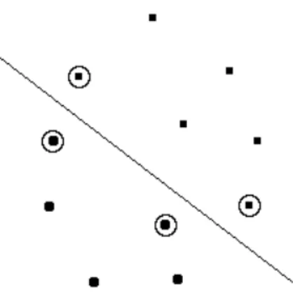
Figure 3: Maximal margin separating hyperplane. Circles mark the support vectors.
Because the hyperplane given by parameters (x, b) is the same as the hy-perplane given by parameters (kx, kb), we can safely bound our search by only considering canonical hyperplanes for which min
i |w Tx
i+b|= 1. It is possible to show that the optimal canonical hyperplane has minimalkwk, and that in or-der to find a canonical hyperplane it suffices to solve the following minimization problem: minimize 1
2w
Twunder the conditions
ci(wTxi+b)≥1, i= 1,2, . . . , n
Using the Lagrangian theory the problem may be trasformed to a certain dual form: maximize Ld(α) = n X i=1 αi− 1 2 n X i,j=1 αiαjcicjxTi xj
with respect to the dual variables α= (α1, α2, . . . , αn) so that αi ≥0 for all i andPn α
This is a classical quadratic optimization problem, also known as aquadratic programme. It mostly has a guaranteed unique solution, and there are efficient algorithms for finding this solution. Once we have found the solution α, the parameters (wo, bo) of the optimal hyperplane are determined as:
wo= n X i=1 αicixi bo= 1 ck −woTxk
wherek is an arbitrary index for whichαk6= 0.
It is more-or-less clear that the resulting hyperplane is completely defined by the training samples that are at minimal distance to it (they are marked with circles on the figure). These training samples are calledsupport vectorsand thus give the name to the method. It is possible to tune the amount of false positives produced by an SVM classifier, by using the so-called soft margin hyperplane and there are also lots of other modifications related to SVM learning, but we shall not discuss these details here as they go out of the scope of this article.
Here’s the summary of the SVM classifier algorithm:
• Training
1. Findαthat solves the dual problem (i.e. maximizesLdunder named constraints)
2. Determinew andbfor the optimal hyperplane. Store the values.
• Classification
1. Given a message x, determine its class as sign(wTx+b).
4
The Algorithms: Practice
In theory there is no difference between theory and practice, but in practice there is.
Now let us consider the performance of the discussed algorithms in practice. To estimate performance, I created the straightforward C++ implementations of the algorithms9, and tested them on the PU1 spam corpus [7]. No optimizations
were attempted in the implementations, and a very primitive feature extractor was used. The benchmark corpus was created a long time ago, so the messages in it are not representative of the spam that one receives nowadays. Therefore the results should not be considered very authoritative. They only provide a general feeling of how the algorithms compare to each other, and maybe some ideas on how to achieve better filtering performance. Consequently, I shall not focus on the numbers obtained in the tests, but rather present some of my conclusions and opinions. The source code of this work is freely available and anyone interested in exact numbers may try running the algorithms himself [23].
9And I used the SVMLight package by Thorsten Joachims [13] for SVM classification. The
4.1
Test Data
The PU1 corpus of e-mail messages collected by Ion Androutsopoulos [7] was used for testing. The corpus consists of 1099 messages, of which 481 are spam. It is divided into 10 parts for performing 10-fold cross-validation (that is, we use 9 of the parts for training and the remaining part for validation of the algorithms). The messages in the corpus have been preprocessed: all the attachments, HTML tags and header fields except Subject were stripped, and words were encoded with numbers. The corpus comes in four flavours: the original version, a version where a lemmatizer was applied to the messages so each word got converted to its base form, a version processed by a “stop-list” so the 100 most frequent English words were removed from each message, and a version processed by both the lemmatizer and the stop-list. Some preliminary tests showed that the algorithms performed better on the messages processed by both the lemmatizer and the stop-list, therefore only this version of the corpus was used in further tests. I would like to note that in my opinion this corpus does not precisely reflect the real-life situation. Namely, message headers, HTML tags and amount of spelling mistakes in a message are among the most precise indicators of spam. Therefore it is reasonable to expect that results obtained with this corpus are worse than what could be in real life. It is good to get pessimistic estimates, therefore the corpus suits nicely for this kind of work. Besides, the corpus is very convenient to deal with thanks to the efforts of its author on preprocessing and formatting the messages.
4.2
Test Setup and Efficiency Measures
Every message was converted to a feature vector with 21700 attributes (this is approximately the number of different words in all the messages of the corpus). An attribute n was set to 1 if the corresponding word was present in a mes-sage, and to 0 otherwise. This feature extraction scheme was used for all the algorithms. The feature vector of each message was given for classification to a classification algorithm trained on the messages of the 9 parts of the corpus, that did not contain the message to be classified.
For every algorithm we counted the numberNS→Lof spam messages incor-rectly classified as legitimate mail (false negatives) and the numberNL→S of le-gitimate messages, incorrectly classified as spam (false positives). LetN = 1099 denote the total number of messages, NS = 481 — the number of spam mes-sages, and NL = 618 — the number of legitimate messages. The quantities of interest are then the error rate
E= NS→L+NL→S N precision
P = 1−E legitimate mail fallout
FL= NL→S
NL andspam fallout
FS = NS→L
Note that the error rate and precision must be consideredrelatively to the case of no classifier. For if we use no spam filter at all we have guaranteed precision NL
N , which is in our case greater than 50%. Therefore we are actually interested in how good is our classifier with respect to this so-called trivial classifier. We shall refer to the ratio of the classifier precision and the trivial classifier precision asgain:
G= P NL/N
=N−NS→L−NL→S NL
4.3
Basic Algorithm Performance
The following table presents the results obtained in the way described above.
Algorithm NL→S NS→L P FL FS G
Na¨ıve Bayes (λ= 1) 0 138 87.4% 0.0% 28.7% 1.56 k-NN (k= 51) 68 33 90.8% 11.0% 6.9% 1.61
Perceptron 8 8 98.5% 1.3% 1.7% 1.75
SVM 10 11 98.1% 1.6% 2.3% 1.74
The first thing that is very surprising and unexpected is the incredible per-formance of the perceptron. After all, it is perhaps the most simple and the fastest algorithm described here. It has even beaten the SVM by a bit, though theoretically SVM should have had better generalization.10
The second observation is that the na¨ıve bayesian classifier produced no false positives at all. This is most probably a feature of my implementation of the algorithm, but, to tell the truth, I could not figure out exactly where the asymmetry came from. Anyway, such a feature is very desirable, so I decided not to correct it. It must also be noted, that when there are less attributes in the feature vector (say, 1000–2000), the algorithm does behave as it should, and has both false positives and false negatives. The number of false positives may then be reduced by increasing theλparameter. As more features are used, the number of false positives decreases whereas the number of false negatives stays approximately the same. With a very large number of features adjusting theλ has nearly no effect, because for most cases the likelihood ratio for a message appears to be either 0 or∞.
The performance of thek-nearest neighbors classifier appeared to be nearly independent of the value of k. In general it was poor, and the number of false positives was always rather large.
As noted in the beginning of this article, a spam filtermay not have false positives. According to this criteria, only the na¨ıve bayesian classifier (in my weird implementation) has passed the test. We shall next try to tune the other algorithms to obtain better results.
4.4
Eliminating False Positives
We need a spam filter with low probability of false positives. Most of the classification algorithms we discussed here have some parameter that may be
10The superiority of SVM showed itself when 2-fold cross-validation was used (i.e. the corpus
was divided into two parts instead of ten). In that case the performance of the perceptron got worse, but SVM performance stayed the same.
adjusted to decrease the probability of false positives at the price of increasing the probability of false negatives. We shall adjust the corresponding parameters so that the classifier has no false positives at all. We shall be very strict at this point and require the algorithm to produce no false positives when trained on any set of parts of the corpus and tested on the whole corpus. In particular, the algorithm should not produce false positives when trained on only one part of the corpus and tested on the whole corpus. It seems reasonable to hope that if a filter satisfies this requirement, we may trust it in real life.
Now let us take a look at what we can tune. The na¨ıve bayesian classifier has theλparameter, that we can increase. Thek-NN classifier may be replaced with thel/kclassifier the numberlmay be then adjusted together withk. The perceptron can not be tuned, so he leaves the competition at this stage. The hard-margin SVM classifier also can’t be improved, but its modification, the soft-margin classifier can. Though the inner workings of that algorithm were not discussed here, the corresponding result will be presented anyway.
The required parameters were determined experimentally. I didn’t actually test that the obtained classifiers satisfied the stated requirement precisely be-cause it would require trying 210different training sets, but I did test quite a lot of combinations, so the parameters obtained must be rather close to the target. Here are the performance measures of the resulting classifiers (the measures were obtained in the same way as described in the previous section)
Algorithm NL→S NS→L P FL FS G
Na¨ıve Bayes (λ= 8) 0 140 87.3% 0.0% 29.1% 1.55 l/k-NN (k= 51,l= 35) 0 337 69.3% 0.0% 70.0% 1.23 SVM soft margin (cost=0.3) 0 101 90.8% 0.0% 21.0% 1.61 It is clear that thel/k-classifier can not stand the comparison with the two other classifiers now. So we throw it away and conclude the section by stating that we have found two more-or-less working spam-filters—the SVM soft margin filter, and the na¨ıve bayesian filter. There is still one idea left: maybe we can combine them to achieve better precision?
4.5
Combining Classifiers
Letf andgdenote two spam filters that both have very low probability of false positives. We may combine them to get a filter with better precision if we use the following classification rule:
Classify messagexas spam if eitherf org classifies it as spam. Otherwise (iff(x) =g(x) =L) classify it as legitimate mail.
We shall refer to the resulting classifier as theunion11off andgand denote
it as f∪g. It may seem that we are doing a dangerous thing here because the
11The name comes from the observation that with a fixed training set, the set of false
positives of the resulting classifier is the union of the sets of false positives of the original classifiers (and the set of false negatives is the intersection of corresponding sets). One may note that we can define a dual operation: the intersection of classifiers, by replacing the wordspamwith the wordlegitimateand vice versa in the definition of the union. The set of all classifiers together with these two operations then form a bounded complete distributive lattice. But that’s most probably just a mathematical curiosity with little practical value
resulting classifier will produce a false positive for a message xif either of the classifiers does. But remember, we assumed that the classifiers f and g have very low probability of false positives. Therefore the probability that either of them does such a mistake is also very low, so union is safe in this sense. Here is the idea explained in other words:
If for a message xit holdsf(x) =g(x) =c, we classifyx as belonging to c (and that is natural, isn’t it?). Now suppose f(x) 6=g(x), for example f(x) =Landg(x) =S. We know thatgis unlikely to misclassify legitimate mail as spam, so the reason that the algorithms gave different results is most probably related to the fact thatf just chose the safe, although the wrong decision. Therefore it is logical to assume that the real class ofxisSrather thanL.
The number of false negatives of the resulting classifier is of course less than of the original ones, because for a messagexto be a false negative off∪git must be a false negative for bothf and g. In the previous section we obtained two classifiers “without” false positives. Here are the performance characteristics of their union:
Algorithm NL→S NS→L P FL FS G
N.B.∪SVM s. m. 0 61 94.4% 0.0% 12.7% 1.68 And the last idea. Lethbe a classifier with high precision (the perceptron or the hard margin SVM classifier for example). We may use it to reduce the probability of false positives of f ∪g yet more in the following way. If f(x) =g(x) =cwe do as before, i.e. classifyxto classc. Now if for a message
xthe classifiersf andggive different results we do not blindly choose to classify
xas spam, but consulthinstead. Becausehhas high precision, it is reasonable to hope that it will give a correct answer. Thus h functions as an additional protective measure against false positives. So we define the following way of combining three classifiers:
Given message x classify it to classc if at least two of the classifiersf, g andhclassify it asc.
It is easy to see that this2-of-3 rule is equivalent to what was discussed.12
Note that though the rule itself is symmetric, the way it is to be applied is not: one of the classifiers must have high precision, and the two others—low probability of false positives.
If we combine the na¨ıve bayesian and the SVM soft margin classifiers with the perceptron this way, we obtain a classifier with the following performance characteristics:
Algorithm NL→S NS→L P FL FS G
2-of-3 0 62 94.4% 0.0% 12.9% 1.68
As you see we made our previous classifier a bit worse with respect to false negatives. We may hope, however, that we made it a bit better with respect to false positives.
12In the terms defined in the previous footnote, this classifier may be denoted as (f∩g)∪
5
The Conclusion
Before I started writing this paper I had a strong opinion, that a good machine-learning spam filtering algorithm is not possible, and the only reliable way of filtering spam is by creating a set of rules by hand. I have changed my mind a bit by now. That is the main result for me. I hope that the reader too could find something new for him in this work.
References
[1] K. Aas, L. Eikvil.Text Categorization: A Survey.1999.
http://citeseer.ist.psu.edu/aas99text.html
[2] N. Cristianini, J. Shawe-Taylor.An Introduction to Support Vector Machines and other kernel-based learning methods.2003, Cambridge University Press.
http://www.support-vector.net
[3] V. Kecman.Learning and Soft Computing.2001, The MIT Press.
[4] S. Haykin.Neural Networks: A Comprehensive Foundation.1998, Prentice Hall.
[5] F. Sebastiani.Text Categorization.
http://faure.iei.pi.cnr.it/~fabrizio/
[6] I. Androutsopoulos et al.Learning to Filter Spam E-Mail: A Comparison of a Naive Bayesian and a Memory-Based Approach.
http://www.aueb.gr/users/ion/publications.html
[7] I. Androutsopoulos et al. An Experimental Comparison of Na¨ıve Bayesian and Keyword-Based Anti-Spam Filtering with Personal E-mail Messages.
http://www.aueb.gr/users/ion/publications.html
[8] P. Graham.A Plan for Spam.
http://www.paulgraham.com/antispam.html
[9] P. Graham.Better Bayesian Filtering.
http://www.paulgraham.com/antispam.html
[10] M. Sahami et al.A Bayesian Approach to Filtering Junk E-Mail [11] H. Drucker, D. Wu, V. Vapnik.SVM for Spam categorization
http://www.site.uottawa.ca/~nat/Courses/NLP-Course/itnn_1999_ 09_1048.pdf
[12] SVM Application List.
http://www.clopinet.com/isabelle/Projects/SVM/applist.html
[13] T. Joachims. Making large-Scale SVM Learning Practical.
Advances in Kernel Methods - Support Vector Learning, B. Schlkopf and C. Burges and A. Smola (ed.), MIT-Press, 1999.
[14] J. Lember.Statistiline ˜oppimine (loengukonspekt).
http://www.ms.ut.ee/ained/LL.pdf
[15] S. Laur.T˜oen¨aosuste leidmine Bayes’i v˜orkudes.
http://www.egeen.ee/u/vilo/edu/2003-04/DM_seminar_2003_II/ Raport/P08/main.pdf
[16] K. Tretyakov, L. Parts.Mitmekihiline tajur.
http://www.ut.ee/~kt/hw/mlp/multilayer.pdf
[17] M. B. Newman.An Analytical Look at Spam.
http://www.vgmusic.com/~mike/an_analytical_look_at_spam.html
[18] C. Eichenberger, N. Fankhauser. Neural Networks for Spam Detection.
http://variant.ch/phpwiki/NeuralNetworksForSpamDetection
[19] M. Vinther.Intelligent junk mail detection using neural networks.
www.logicnet.dk/reports/JunkDetection/JunkDetection.pdf
[20] InfoAnarchy Wiki: Spam.
http://www.infoanarchy.org/wiki/wiki.pl?Spam
[21] S. Mason.New Law Designed to Limit Amount of Spam in E-Mail.
http://www.wral.com/technology/2732168/detail.html
[22] http://spam.abuse.net/
[23] Source code of the programs used for this article is available at
http://www.ut.ee/~kt/spam/spam.tar.gz