Feature Induction and Network Mining with Clustering Tree Ensembles

Feature Induction and Network Mining with

Clustering Tree Ensembles

Konstantinos Pliakos and Celine Vens

KU Leuven, Campus KULAK, Department of Public Health and Primary Care, Etienne Sabbelaan 53, Kortrijk 8500, Belgium

[email protected], [email protected],

Abstract. The volume of data generated and collected using modern technologies grows exponentially. This vast amount of data often follows a complex structure, and the problem of efficiently mining and analyz-ing such data is crucial for the performance of various machine learnanalyz-ing tasks. Here, a novel data mining framework for unsupervised learning tasks is proposed based on decision tree learning and ensembles of trees. The proposed approach introduces an informative feature representation and is able to handle data diversity and complexity. Moreover, a new scheme is proposed based on the aforementioned approach for mining interaction data. These data are often modeled as homogeneous or het-erogeneous networks and they are present in various fields, such as social media, recommender systems, and bioinformatics. The learning process is performed in an unsupervised manner, following also the inductive setup. The experimental evaluation confirms the effectiveness of the proposed approach.

Keywords: tree-ensembles, extremely randomized trees, tree-embedding, network mining

1

Introduction

Nowadays, a great advance in data acquisition and feature construction meth-ods is witnessed. Due to modern technological advances, huge amounts of data are generated in terms of both cardinality (i.e., the number of samples) and dimensionality (i.e., the number of features that describe each sample). These data often follow more complex structures, combining information from multiple sources. One example that is often encountered is interaction data. Instead of one set of objects described by a set of features, interaction data is characterized by two sets of objects, each described by its own set of features. Interaction data is omni-present: in social network analysis, recommender systems, ecology (habi-tat modeling), bioinformatics (gene expression analysis, drug response analysis, predicting drug-target reactions), technology-enhanced education, etc. Further-more, as the volume of data grows, problems such as the existing noise in the data or the missing values in some datasets remain. To this end, methods that can handle the aforementioned issues and succeed in mining complex patterns in big datasets are indisputably needed.

During the last years, an interest was witnessed in leveraging the mining of complex patterns by mapping the data to different feature spaces. This way, the performance of machine learning algorithms was improved. Most of the devel-oped methods were based on kernel learning [1, 2], mainly due to the very good performance of Support Vector Machines (SVMs) [3]. However, these methods are often characterized by high computational costs and limited flexibility as one should compute and handle the whole Gram matrix. Many of these kernel-based methods have also been developed in a transductive setup where test instances are available during the training phase [1].

There are several studies where new features are constructed inductively us-ing clusterus-ing techniques or decision tree learnus-ing. Most of the recently developed feature construction methods were developed for supervised learning tasks. In [4], a feature induction method based on random forests [5] was proposed. It was based on a metric transformation that mapped the identity of the tests per-formed in each node of a decision tree to a feature indicator. Feature vectors were generated by concatenating all the features corresponding to each tree in the forest and they were further encoded using hashing. A similar transforma-tion of the data, using a set of random clustering forests was proposed in [6, 7] for visual codebook construction. In particular, the features were generated by randomized trees. The data encoding was based only on the indices of the leaves where a data sample ends up. The approach leads to a high dimensional, sparse binary coding. In [8], a label-specific feature scheme for multi-label clas-sification was proposed. For each label, a distinct feature set was constructed by clustering the label’s positive and negative instances (separately), and then calculating the distances of each instance to the obtained cluster centroids. This way, the predictive performance of a classifier trained for that specific label was increased.

Here, we focus on developing a feature representation using tree ensembles. The main goal is to leverage unsupervised machine learning tasks, such as clus-tering or information retrieval. Decision tree induction algorithms [9, 10] are among the most popular data mining algorithms. They have been applied ex-tensively in many fields such as systems biology [11] or social media analysis [12]. The interpretability of the models they produce is among the main advantages of these methods, making them transparent and understandable to human experts, also leveraging knowledge discovery. Other advantages include their scalability from a computational point of view and their fair predictive accuracy. Combin-ing them with ensemble methods [13, 5] improves their predictive performance and provides state-of-the-art results.

Motivated by [4], here we propose an unsupervised framework for feature construction based on tree ensembles and specifically Extremely Randomized Trees [14], hereafter denoted asERT. In particular, the nodes of each decision tree of the ensemble are treated as clusters, containing all the samples that fall into that tree node. Next, binary feature vectors are generated, where each component represents the presence or absence of a sample in a cluster (node). The new features are generated in an inductive manner (i.e., the test samples

are not needed during learning). Different from [4], the learning procedure is performed in an unsupervised manner. In addition, the employment of dimen-sionality reduction techniques [15, 16] is studied and the efficiency in detecting an underlying manifold over complex data is tested.

Furthermore, the proposed data representation approach is extended towards interaction data. Relations between entities that interact with each other such as user-item relations in recommender systems or drug-patient interactions in medicine are often represented by networks (here, equally referred to as graphs). Generally, there are two types of networks, homogeneous that model samples of the same type (e.g., protein-protein network) and bi-partite modeling samples of different type (e.g., drug-protein network). Despite the continuous rising in the amount of available data, usually we have only a very partial knowledge of these networks [17]. Both supervised and unsupervised machine learning methods have been used to complete a partially known network or to reveal unprecedented knowledge by extracting existing patterns from it [18, 19]. There are mainly two methodologies to apply a learning technique in the aforementioned framework, the local approach [20] and the global one [21]. Following the local approach one should first decompose the data into separate (traditional) feature vector repre-sentations, solve each representation ’s learning task independently, and combine the results. In the global approach, the learning technique is adapted so that it can handle the structured representation directly. In [17], the global approach was based on building a global representation of the network and then treat the interaction prediction problem as a binary classification task. Here, a method is proposed that combines these two approaches in a unified framework. More pre-cisely, the aforementioned feature induction approach based onERT is applied on each set of the two interacting entities separately (local part), producing two new high-dimensional sparse representations. Next, after transferring the two sets to lower dimensional spaces we combine the two separate low-dimensional feature representations, building this way a global representation of the network. To this end, it can be concluded that the proposed approach yields a new global network representation that is more informative and computationally more ef-ficient. The experimental results demonstrate the effectiveness of the proposed approach.

The outline of the paper is as follows. In Section 2, the proposed approach is described in detail. The experimental evaluation is presented in Section 3. Conclusions are drawn and topics of future research are discussed in Section 4.

2

Method

2.1 Learning using Extremely Randomized Trees

Decision trees are typically constructed with a top-down induction method. Starting from the root node that is associated with the complete training set, the nodes are recursively split by applying a test to one of the features. In order to find the best split, all features and their corresponding split points are consid-ered and a split quality criterion is evaluated. In supervised learning tasks, this

criterion is often information gain (classification), or variance reduction (regres-sion). When the data contained in a node is pure w.r.t. the target, or when some other stopping criterion holds, the node becomes a leaf node and a prediction is assigned to it. This prediction is the majority class assigned to the training instances in the leaf for classification, or the average of their target values for regression. The prediction for test instances is obtained by sorting them through the tree into a leaf node. In this work, the decision tree learners employed are set in the Predictive Clustering Tree (PCT) [10] framework, adopting the hier-archical clustering view of decision trees. PCTs are constructed by maximally reducing intra-cluster variance at each split. By computing the variance over the feature set, rather than the target, PCTs can be applied to (unsupervised) clustering tasks.

Since decision trees often have a large variance, their predictive performance can be improved by having several trees returning an aggregated prediction. Such a collection of decision trees is called an ensemble, and several instances of ensembles exist. In this work, we consider the ensemble method of Extremely Randomized Trees (ERT) [14, 22]. The ERT algorithm builds an ensemble of un-pruned decision trees following the traditional top-down procedure. In an ERT ensemble, each tree is constructed by considering only a random set of split candidates at each node. More precisely, a random subset of features is picked, and for each feature, a random split point is picked. From these candidates, the candidate yielding the best value for the split criterion is chosen. The growing of each tree is stopped when the tree is fully grown (i.e., one sample in each leaf) or a criterion has been reached (e.g., maximum depth, minimum number of samples to split, etc.). The rationale behind the ERT algorithm is that the ex-plicit randomization of the splitting threshold and attribute in combination with ensemble averaging reduces bias-variance more strongly than the randomization performed by other methods. ERT was shown to have a better predictive perfor-mance than the more popular Random Forests [14] and it is also computationally less expensive due to the simplicity of the node splitting procedure.

2.2 Feature construction with extremely randomized trees

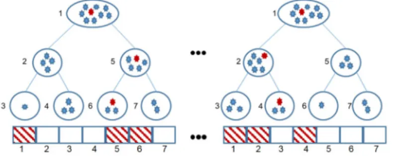
A new feature set is generated by applying ERT on the initial feature set, as follows. The nodes of each tree in the ERT setting, C = {c1, c2,· · ·, c|C|} are

treated as clusters containing all the samples that fall into them traversing the tree. Clearly, there is no point into including the root nodes in the procedure. LetX∈ <|S|×|M|_{be the dataset andF∈ <}|S|×|C|_{the induced feature set, where}

|S|, |M| and|C| correspond to the number of samples, the number of original features, and the number of induced features of the dataset, respectively. Next, the clusters cj ∈C are treated as features of the feature set F. Each fij ∈ F

equals to 1 if the sample i ∈ S is contained in the cluster (node) cj and 0

otherwise. The proposed approach is coined as ERCP (Extremely Randomized Clustering tree-Paths). In Fig. 1, the feature induction approach is shown.

The proposed feature representation is rationally more informative than the original one. Due to the feature selection mechanism of the ERT, features that

contain redundant information are not included in the procedure (i.e., no split occurs on these features). The induced features are generated by computing clus-terings over the whole dataset and therefore information from the whole instance space is exploited. Samples that are outliers in the dataset can be discriminated easily, as splitting an outlier from the rest of the dataset rationally leads to large variance reduction. In addition, regions of the instance space with high variance will lead to longer paths in the trees, thereby making the procedure adaptive towards the difficulty of the instances considered. Moreover, one can control the growing of the trees by setting specific stopping criteria.

At this point, it has to be noted that a similar encoding could be produced by any hierarchical clustering method. However, the employment of ERT is ben-eficial. First, ERT is a tree ensemble method, and therefore it is robust to small perturbations in the data. It is also robust to non-informative or noisy features due to the implicit feature selection mechanism. This way, the generated feature representation is considered more noise invariant. Moreover, another advantage is that the tree ensembles can generally treat both numerical and non-numerical values, making the method more easily applied and robust. In addition to that, in contrast to many other methods, it offers a natural way to deal with missing values by distributing instances with a missing split value over all branches or by selecting at random one branch to follow. Other advantages of the proposed approach is that it is parameter-free and it is performed in an inductive manner. After the training, the model can handle any new data without any need of the training set. Furthermore, it is expected that a greater number of examples will lead to bigger trees in the forest. The proposed representation will be therefore larger but also very sparse. This way, the application of our approach to modern online systems as well as systems that handle large scale data is feasible.

Fig. 1.Illustration of the proposed approach. The example associated with the induced feature vector is depicted as red.

2.3 Mining Interaction Data

As mentioned before, the relations between two entities that interact with each other are often represented as a network (here, equally referred to as a graph).

LetGdefine a network with two finite sets of nodes Nr={nr1,· · ·, nr|Nr|} and

Nq ={nq1,· · ·, nq|Nq|}. Each node of the network is described by a feature

rep-resentation. The network corresponds to a bipartite graph over the two sets of nodesNrandNq. The interactions betweenNrandNqare modeled as edges

con-necting the nodes and are represented in the adjacency matrixY∈ <|Nr|×|Nq|_.

Every itemy(i, j)∈Yis equal to 1 if an interaction between itemsnri andnqj

exists and 0 otherwise. Homogeneous graphs defined on only one type of nodes can be obtained as a particular case of the aforementioned general framework by considering two identical sets of nodes (i.e.,Nr=Nq).

In the proposed approach the bipartite graph is first decomposed into two separate sets of nodes. For example in a drug-protein interaction network one has a set of nodes corresponding to drugs and one corresponding to proteins. Each set of nodes Nr or Nq is represented by a feature set Xr ∈ <|Nr|×|Mr|

or Xq ∈ <|Nq|×|Mq|, respectively. Next, two feature sets Fr ∈ <|Nr|×|Cr| and

Fq ∈ <|Nq|×|Cq| are induced by applying ERCP onXr and Xq respectively, as

described in Sec. 2.2. The new high dimensional feature representation of the nodes is then transferred to a lower dimensional spaced(dr |Cr|, dq |Cq|).

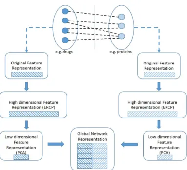
This transformation could be performed by embedding the data into a linear or non-linear subspace of lower dimensionality. Although many techniques exist, here the most popular Principal Components Analysis (PCA) was employed. By applying PCA the inductive setup of the method is maintained. Next, a global data representation is built as the cartesian product of the two feature spaces. More precisely, a feature vector is generated for each pair of nodes as the concatenation of the feature vectors corresponding to the nodes of each pair. To this end, a global representationF0is yielded, whereF0∈ <k|Nr|∗|Nq|k×k|dr|+|dq|k_.

In Fig. 2, the proposed model for mining interaction data is displayed.

3

Experimental Evaluation

3.1 Datasets

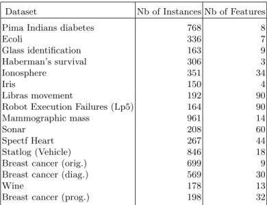
The evaluation procedure of the proposed approach starts by employing some well-known datasets from UCI repository [23] in order to reveal the global po-tential of our approach. The evaluation continues by employing more complex datasets and specifically two datasets that correspond to homogeneous biological networks. Next, the evaluation of the interaction data mining approach (Sec. 2.3) follows. Including several datasets from various fields contributes in avoiding any biased conclusions and revealing the robustness of our method. The labels con-tained in these datasets were used only for evaluation purposes and were not included in any part of the learning process. In Table 1, further information about the used datasets is provided. A pre-processing step was also introduced as in [4]. In particular, the data have been whitened by normalizing all features to have zero mean and unit standard deviation. Non-binary classification tasks were transformed into binary ones by considering the majority class versus all the others or by grouping the classes in two sets of balanced size. Despite the fact that tree-ensembles do not require any pre-processing of the data, in order

Fig. 2.A description of the proposed interaction data representation model.

to compare the proposed feature representation to the original one the missing values were replaced by the features ’s average and the nominal features in some datasets were transformed into a set of binary ones using one-hot encoding. This way, algorithms that can not handle missing values (e.g., k-NN, k-means) can be applied on both data representations (original features, induced features) for comparison purposes.

In order to prove the efficiency of the proposed feature representation ap-proach on more complex data structures, 5 interaction prediction datasets [17] were also introduced. They are interaction datasets representing homogeneous and heterogeneous biological networks. In particular:

– Metabolic network (MN) [24]. This homogeneous network consists of 668 S. cerivisiae enzymes and the connections represent the catalysation of succesive reactions between two enzymes. The enzymes are originally rep-resented by 325 features. They are a set of expression data, phylogenetic profiles and localization data.

– Protein-protein interaction network (PPI) [25]. This homogeneous network contains interactions between 984 S. cerivisiae proteins. The input features are also a set of expression data, phylogenetic profiles and localiza-tion data.

– E. coli regulatory network (ERN) [26]. This heterogeneous network consists of 179256 pairs of 154 transcription factors (TF) and 1164 genes of E. coli (154×1164 = 179256). The feature vectors that represent the two sets consist of 445 expression values.

Table 1.The datasets used in the evaluation procedure. Dataset Nb of Instances Nb of Features

Pima Indians diabetes 768 8

Ecoli 336 7 Glass identification 163 9 Haberman’s survival 306 3 Ionosphere 351 34 Iris 150 4 Libras movement 192 90

Robot Execution Failures (Lp5) 164 90

Mammographic mass 961 14

Sonar 208 60

Spectf Heart 267 44

Statlog (Vehicle) 846 18

Breast cancer (orig.) 699 9

Breast cancer (diag.) 569 30

Wine 178 13

Breast cancer (prog.) 198 32

– S. cerevisiae regulatory network (SRN) [27]. This heterogeneous net-work is composed by interactions between TFs and their target S. cerevisiae genes. It is composed of 205773 pairs of 1821 genes and 113 TFs. The input features are 1685 expression values. For genes, motifs features were concate-nated to the expression values yielding feature vectors of 9884 values. – Drug–protein interaction network (DPI) [28]. In this heterogeneous

network a drug is connected with a protein when the drug targets the protein. This network contains interactions between 683 proteins and 1779 drugs, yielding a set of 1215057 pairs. The input feature vectors represent the pres-ence or abspres-ence of 660 chemical substructures for each drug, and the prespres-ence or absence of 876 PFAM domains for each protein.

3.2 Experimental Results

Although we target unsupervised learning tasks, datasets with known class la-bels were used in order to better evaluate the proposed feature construction technique, denoted as Extremely Randomized Clustering tree Paths (ERCP). In particular, the class labels were used only as ground truth during evaluation and were disregarded during the learning phase. The performance of a k-NN algorithm applied on the induced features generated by ERCP was measured and compared to the performance of k-NN applied on the original data. The underlying idea is that instances with the same class should get a similar feature representation, even though that class information is not used in the construction of the features.

Furthermore, totally random trees embedding [6] was also used in compar-ison. It was employed as an unsupervised transformation of the data, using a forest of Extremely Random Clustering trees (ERC) with a single random split candidate per node. In ERC the data are transformed using only the indices of the leaves of each tree. Similar to our approach, ERT was also chosen as the base estimator.

The number of trees used in the ensembles for all the compared methods was set to 300. At that number, the Gram matrix induced on the new features converged in the supervised setting [4]. The number of the features selected as splitting candidates (Tf) was set equal to the square root of the number of

original features (Tf =

p

|M|). The variance over the feature set was computed as the sum of the variances over the individual features. All trees were unpruned, and the minimal number of instances a leaf has to cover was set equal to 3. As for k-NN, the 3 nearest neighbors were considered (k = 3). Experiments selecting other numbers of nearest neighbors or splitting candidates (Tf) were

also performed without showing a different trend. The evaluation was performed in a 10-fold cross validation (10 CV) scheme.

The evaluation measures that were employed were the common accuracy and the area under the receiver operating characteristic curve (AUROC). A ROC curve is defined as the true positive rate (TPR) against the false positive rate (FPR) at various thresholds. Alternatively, the true-positive rate is known as sensitivity and the false-positive rate as (1 - specificity).

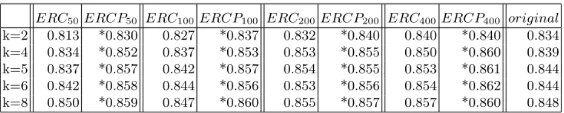
As it is reflected in Tables 2 and 3 the proposed methodERCP outperforms ERC in terms ofAU ROC. For each dataset, the best result is indicated with ∗. Furthermore, both tree-based ensemble methods succeed in generating a bet-ter feature representation set than the original one. More precisely, the average AU ROC results forERCP andERC are 0.854 and 0.844, respectively. On the original set the average drops to 0.836. Further experiments were performed us-ing different number of trees in the ensemble and different number of nearest neighbors. The obtained results, that are shown in Table 3, reaffirm the perfor-mance of the proposed approach. When it comes to accuracy the same behavior was witnessed as the average rates are 0.831, 0.827, and 0.824 for the ERCP, ERC, and the original set respectively.

In addition to k-NN, k-means was employed extending the evaluation of the proposed method to a clustering setting. Although there are many clustering algorithms, k-means was selected out of simplicity. The number of clusters was set equal to 2 as all the datasets contain 2 classes. The evaluation metric that was used was the adjusted Rand index [29], measuring the similarity between the ground truth class assignments and the clustering algorithm assignments. The compared approaches correspond to different dimensional spaces, making the application of an evaluation metric based on the distances or the variances of the clusters difficult. Although the labels assigned to the samples by unsupervised clustering are without intrinsic meaning, the rational idea is that samples with the same ground truth are similar and therefore should be grouped together. As it is reflected in Table 4, the proposed method ERCP outperforms the other

Table 2.AU ROCmeasures for the compared approaches.

Data original ERC ERCP

Pima Indians diabetes *0.767 0.726 0.731

Ecoli *0.966 0.965 0.965 Glass identification 0.805 0.823 *0.871 Haberman’s survival 0.629 0.609 *0.630 Ionosphere 0.897 0.937 *0.957 Iris *1 *1 *1 Libras movement 0.753 *0.801 0.735 Robot Execution Failures (Lp5) 0.915 0.886 *0.968 Mammographic mass 0.791 *0.795 0.791

Sonar 0.718 0.713 *0.734

Spectf Heart 0.707 0.748 *0.779 Statlog (Vehicle) 0.981 *0.986 0.971 Breast cancer (orig.) 0.982 *0.983 *0.983 Breast cancer (diag.) 0.984 *0.985 0.977

Wine 0.970 *0.991 0.973

Breast cancer (prog.) 0.503 0.546 *0.590 Average 0.836 0.844 *0.854

Nb wins 3 7 *9

Average ranks 2.31 1.94 *1.75

Table 3.AverageAU ROCwith different numbers of trees and nearest neighbors.

ERC50ERCP50 ERC100ERCP100 ERC200 ERCP200 ERC400 ERCP400 original

k=2 0.813 *0.830 0.827 *0.837 0.832 *0.840 0.840 *0.840 0.834 k=4 0.834 *0.852 0.837 *0.853 0.853 *0.855 0.850 *0.860 0.839 k=5 0.837 *0.857 0.842 *0.857 0.854 *0.855 0.853 *0.861 0.844 k=6 0.842 *0.858 0.844 *0.856 0.853 *0.856 0.854 *0.862 0.844 k=8 0.850 *0.859 0.847 *0.860 0.855 *0.857 0.857 *0.860 0.848

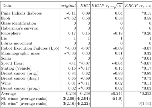
Table 4.Adjusted Rand index results for the compared approaches. Data original ERC ERCP Tf=p|M| ERCP (Tf= 1)

Pima Indians diabetes ?0.11 0.09 0.04 *0.15

Ecoli ?*0.62 0.58 0.58 0.58 Glass identification 0 0 0 0 Haberman’s survival 0 0 0 0 Ionosphere 0.17 0.15 ?0.18 *0.20 Iris 1 1 1 1 Libras movement 0 0 0 0

Robot Execution Failures (Lp5) *-0.03 -0.07 ?0.09 -0.07 Mammographic mass ?*0.36 0.30 0.31 0.32

Sonar 0 0 0 *0.01

Spectf Heart -0.1 *-0.07 ?-0.04 *-0.07 Statlog (Vehicle) 0.15 ?*0.17 0.15 *0.17 Breast cancer (orig.) 0.84 0.82 ?0.89 *0.89 Breast cancer (diag.) 0.65 ?0.69 0.68 *0.73

Wine 0.01 ?*0.11 0.02 *0.11

Breast cancer (prog.) 0.02 ?*0.03 0.02 *0.03

Average 0.238 0.238 ?0.244 *0.253

Nb wins?(average ranks) 3(2.06) 4(2.04) 4(1.9) -Nb wins* (average ranks) 3(2.16) 4(2.22) - 9(1.63)

comparing approaches for both Tf =

p

|M| and Tf = 1. It is interesting to

note that the best results in clustering (k-means) are obtained with Tf = 1

(totally randomized tree-paths, as in ERC). The best results among the ERC, ERCP

Tf=

√

|M|, and the originalfeatures are reported with?. The best results

among theERC,ERCPTf=1, and theoriginalfeatures are reported with∗. It

has to be mentioned that optimizing some parameters for each dataset was not part of the study performed here, even though it could possibly lead to better results.

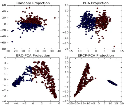
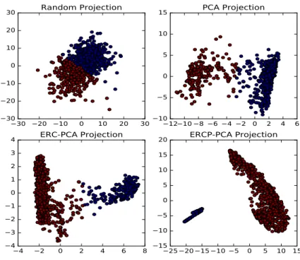
In Figs. 3 and 4, a visualization of PPI and MN datasets (homogeneous networks) is displayed by projecting the data in a 2-dimensional (2D) space using PCA. Other linear or non-linear techniques such as the t-SNE [30] could have been used but the common PCA was chosen out of simplicity. As reflected in the Figs. 3 and 4, the generated data distribution after applying PCA to the original data fails to detect any underlying manifold and it is similar to a common random projection, especially for the MN dataset. In the case of ERC, two clusters seem to appear, however it is not clear where to dichotomize the data. Finally, the application of PCA to the ERCP-induced feature space leads to a more informative distribution and shows two clearly disconnected clusters. The two clusters have been color coded with colors blue and red, and the same coding scheme was applied in the other graphs. For the PPI dataset, a Gene Ontology Enrichment analysis was performed using YeastMine [31] in

30 20 10 0 10 20 30 40 80 60 40 20 0 20 40 60

Random Projection

PCA Projection

ERC-PCA Projection

ERCP-PCA Projection

Fig. 3. MN network data projection. Upper left a totally random projection of the data is depicted. Upper right the PCA projection of the original data is shown. Down left the PCA projection of theERC feature representation is displayed. Down right the PCA projection of theERP Cis displayed.

order to assign a biological interpretation to the obtained clusters. Using the complete set of proteins as background, it turns out that the bigger cluster (red) is enriched with proteins localized in the nucleus (p=3.26e-60), while the smaller cluster is enriched with cytoplasm cellular component annotations (p=0.038). It is concluded that ERCP succeeds in providing a more informative feature representation for complex datasets.

Next, the experimental evaluation of the proposed interaction data mining scheme is presented. The global representation was constructed as described in Sec. 2.3. It consists of all the possible pairs of network nodes. For evaluation purposes, the known interactions or non-interactions between these nodes were coded as 1 and 0, respectively. They were used as ground truth without taking part in the learning process. Then, the performance of a k-NN algorithm applied to that global representation was measured. The global network representation based on the proposed approach that was described in Sec. 2.3 is referred to as MID-CT (Mining Interaction Data with Clustering Trees). The global represen-tation based on the original features is coined as Global Network Represenrepresen-tation (GNR) and a global representation based on the original features and PCA is coined as GNR-PCA. More specifically, in GNR-PCA only PCA is applied on the original features of each node-set. Here, the number of components that were kept was set equal to the square root of the original features (p|M|). In Table 5, the accuracy results of k-NN for the first nearest neighbor (1-NN) as well as the

30 20 10 0 10 20 30 30 20 10 0 10 20 30

Random Projection

PCA Projection

ERC-PCA Projection

ERCP-PCA Projection

Fig. 4. PPI network data projection. Upper left a totally random projection of the data is depicted. Upper right the PCA projection of the original data is shown. Down left the PCA projection of theERC feature representation is displayed. Down right the PCA projection of theERP Cis displayed.

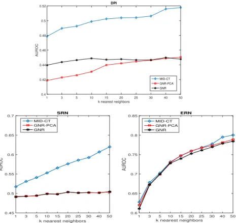
sizes of the compared representations are shown. In Fig. 5, the AUROC values for different numbers of nearest neighbors are shown. As it is reflected, the MID-CT clearly outperforms the other approaches. It is also shown that the results are improved using high values of k in k-NN. To this end, it could be deducted that the representation yielded by our approach is characterized by more pure neighborhoods. Moreover, it has to be mentioned that MID-CT yields a compu-tationally much more efficient representation than GNR as it reduces the size of the two interaction sets before the final construction of the global representation. This way, a global network representation of much less dimensions is obtained.

Table 5.Accuracy results (1-NN) for the compared approaches. Dataset Size of GNR Size of MID-CT GNR GNR-PCA MID-CT DPI(drug-protein) 1215057×1536 1215057×56 0.7655 0.7757 *0.9180 SRN(genes-TF) 205773×11569 205773×140 0.5495 0.5510 *0.9293 ERN(genes-TF) 179256×890 179256×42 0.9415 0.9515 *0.9719

1 3 5 10 15 20 25 30 40 50 k nearest neighbors 0.4 0.42 0.44 0.46 0.48 0.5 0.52 AUROC DPI MID-CT GNR-PCA GNR 1 3 5 10 15 20 25 30 40 50 k nearest neighbors 0.45 0.5 0.55 0.6 0.65 0.7 AUROC SRN MID-CT GNR-PCA GNR 1 3 5 10 15 20 25 30 40 50 k nearest neighbors 0.6 0.65 0.7 0.75 0.8 0.85 AUROC ERN MID-CT GNR-PCA GNR

Fig. 5.AUROC results for different numbers of nearest neighbors.

4

Conclusions and Future work

In this paper, we proposed an efficient feature representation framework based on decision tree ensembles for unsupervised learning tasks. In particular, we employed Extremely Randomized Trees in an unsupervised manner, by evalu-ating the quality of a split on the feature space, rather than the target space. By registering the tree nodes that are encountered by a given sample, a high-dimensional, very sparse feature space is obtained. The proposed approach is inductive and can handle complex data structures. Moreover, we proposed a new scheme based on the aforementioned approach for mining interaction data orga-nized as heterogeneous networks. Finally, we empirically evaluated the proposed data representation using UCI datasets as well as more complex datasets repre-senting interaction networks. The effectiveness of the approach was confirmed by showing improved performance when a mining algorithm or data visualisation step is applied on the obtained feature representation.

Possible topics for future research include the application of various machine learning algorithms to the generated feature representation or the development of an efficient weighing scheme, assigning a different weight to each tree-node of the ensemble. This way, the information contained in each generated feature will be distilled.

Acknowledgments

The authors acknowledge the Research Fund KU Leuven. They also want to thank Lieven Thorrez for input and feedback on the biological interpretation of the visualization results.

References

1. Lanckriet, G. R., Cristianini, N., Bartlett, P., Ghaoui, L. E., Jordan, M. I.: Learn-ing the kernel matrix with semidefinite programmLearn-ing. Journal of Machine learnLearn-ing research, 5, 27–72 (2004)

2. Shawe-Taylor, J., Cristianini, N.: Kernel methods for pattern analysis. Cambridge university press (2004)

3. Burges, C. J.: A tutorial on support vector machines for pattern recognition. Data Mining and Knowledge Discovery, 2, 2, 121–167 (1998)

4. Vens, C., Costa, F.: Random forest based feature induction. in Proc. IEEE 11th Int. Conf. on Data Mining (ICDM), 744–753 (2011)

5. Breiman, L.: Random forests. Machine learning, 45, 1, 5–32 (2001)

6. Moosmann, F., Triggs, B., Jurie, F.: Fast discriminative visual codebooks using randomized clustering forests. in Proc. 20th Conf. on Neural Information Processing Systems (NIPS), 985-992 (2006)

7. Moosmann, F., Triggs, B., Jurie, F.: Randomized clustering forests for image clas-sification. in IEEE Trans. on Pattern Analysis and Machine Intelligence, 30, 9, 1632–1646 (2008)

8. Zhang, M., Wu, L.: LIFT: Multi-label learning with label-specific features. IEEE Trans. on Pattern Analysis and Machine Intelligence, 37, 1, 107–120 (2015) 9. Blockeel, H., De Raedt, L.: Top-down induction of first-order logical decision trees.

Artificial intelligence, 101, 1, 285–297 (1998)

10. Blockeel, H., De Raedt, L., Ramon, J.: Top-Down Induction of Clustering Trees. in Proc. 15th Int. Conf. on Machine Learning, 55–63 (1998)

11. Geurts, P., Irrthum, A., Wehenkel, L.: Supervised learning with decision tree-based methods in computational and systems biology. Molecular Biosystems, 5, 12, 1593– 1605 (2009)

12. Agichtein, E., Castillo, C., Donato, D., Gionis, A., Mishne, G.: Finding high-quality content in social media. in Proc. ACM Int. Conf. on Web Search and Data Mining, 183–194 (2008)

13. Kocev, D., Vens, C., Struyf, J., Dˇzeroski, S.: Tree ensembles for predicting struc-tured outputs. Pattern Recognition, 46, 3, 817–833 (2013)

14. Geurts, P., Ernst, D., Wehenkel, L.: Extremely randomized trees. Machine learning, 63, 1, 3–42 (2006)

15. Yan, S., Xu, D., Zhang, B., Zhang, H. J., Yang, Q., Lin, S.: Graph embedding and extensions: a general framework for dimensionality reduction. in IEEE trans. on Pattern Analysis and Machine Intelligence, 29, 1, 40–51 (2007)

16. Van Der Maaten, L., Postma, E., Van den Herik, J.: Dimensionality reduction: a comparative review. Journal of Machine Learning Research, 10, 66–71 (2009) 17. Schrynemackers, M., Wehenkel, L., Babu, M. M., Geurts, P.: Classifying pairs

with trees for supervised biological network inference. Molecular BioSystems, 11, 8, 2116–2125 (2015)

18. Maetschke, S. R., Madhamshettiwar, P. B., Davis, M. J., Ragan, M. A.: Supervised, semi-supervised and unsupervised inference of gene regulatory networks. Briefings in Bioinformatics, 15, 2, 195-211 (2014)

19. Stojanova, D., Ceci, M., Malerba, D., Dzeroski, S.: Using PPI network autocor-relation in hierarchical multi-label classification trees for gene function prediction. BMC bioinformatics, 14, 1, 285 (2013)

20. Bleakley, K., Biau, G., Vert, J.P.: Supervised reconstruction of biological networks with local models. Bioinformatics, 23, 13, i57–i65 (2007)

21. Vert, J.P., Qiu, J., Noble, W.S.: A new pairwise kernel for biological network inference with support vector machines. BMC bioinformatics, 8, 10, 1 (2007) 22. Kocev, D., Ceci, M.: Ensembles of extremely randomized trees for multi-target

regression. Discovery Science, 86–100 (2015)

23. Asuncion, A., Newman, D.: UCI machine learning repository. [Online] Available: http://www.ics.uci.edu/ mlearn/MLRepository.html

24. Yamanishi, Y., Vert, J. P., Kanehisa, M.: Supervised enzyme network inference from the integration of genomic data and chemical information. Bioinformatics, 21, Suppl. 1, i468-i477 (2005)

25. Von Mering, Ch., Krause, R., Snel, B., Cornell, M., Oliver, S. G., Fields, S., Bork, P.: Comparative assessment of large-scale data sets of protein–protein interactions. Nature, 417, 6887, 399–403 (2002)

26. Faith, J. J., Hayete, B., Thaden, J. T., Mogno, I., Wierzbowski, J., Cottarel, G., Kasif, S., Collins, J. J., Gardner, T. S.: Large-scale mapping and validation of Es-cherichia coli transcriptional regulation from a compendium of expression profiles. PLoS biol, 5, 1, e8 (2007)

27. MacIsaac, K. D., Wang, T., Gordon, D. B., Gifford, D. K., Stormo, G. D., Fraenkel, E.: An improved map of conserved regulatory sites for Saccharomyces cerevisiae. BMC Bioinformatics, 7, 1, 1 (2006)

28. Yamanishi, Y., Pauwels, E., Saigo, H., Stoven, V.: Extracting sets of chemical substructures and protein domains governing drug-target interactions. Journal of chemical information and modeling, 51, 5, 1183–1194 (2011)

29. Hubert, L., Arabie, P.: Comparing partitions. Journal of classification, 2, 1, 193– 218 (1985)

30. Van Der Maaten, L., Hinton, G.: Visualizing data using t-SNE. Journal of Machine Learning Research, 9, 2579–2605 (2008)

31. Cherry, J. M., Hong, E. L., Amundsen, C., Balakrishnan, R., Binkley, G., Chan, E. T., Christie, K. R., Costanzo, M. C., Dwight, S. S., Engel, S. R., Fisk, D. G., Hirschman, J. E., Hitz, B. C., Karra, K., Krieger, C. J., Miyasato, S. R., Nash, R. S., Park, J., Skrzypek, M. S., Simison, M., Weng, S., Wong, E. D.: Saccha-romyces Genome Database: the genomics resource of budding yeast. Nucleic Acids Res. (2012)