CIVIL ENGINEERING
Vector machine techniques for modeling
of seismic liquefaction data
Pijush Samui
*
Centre for Disaster Mitigation and Management, VIT University, Vellore 632014, India
Received 10 September 2013; revised 3 December 2013; accepted 24 December 2013 Available online 22 January 2014
KEYWORDS
Support Vector Machine; Least Square Support Vector Machine;
Relevance Vector Machine; Liquefaction;
Probability
Abstract This article employs three soft computing techniques, Support Vector Machine (SVM);
Least Square Support Vector Machine (LSSVM) and Relevance Vector Machine (RVM), for pre-diction of liquefaction susceptibility of soil. SVM and LSSVM are based on the structural risk min-imization (SRM) principle which seeks to minimize an upper bound of the generalization error consisting of the sum of the training error and a confidence interval. RVM is a sparse Bayesian ker-nel machine. SVM, LSSVM and RVM have been used as classification tools. The developed SVM, LSSVM and RVM give equations for prediction of liquefaction susceptibility of soil. A comparative study has been carried out between the developed SVM, LSSVM and RVM models. The results from this article indicate that the developed SVM gives the best performance for prediction of liq-uefaction susceptibility of soil.
Ó2014 Production and hosting by Elsevier B.V. on behalf of Ain Shams University.
1. Introduction
There is a lot of engineering problems that require the analysis of uncertain and imprecise information. Generally, the devel-opment of proper model to explain past behaviors or predict future ones is a difficult task due to incomplete understanding of the problem. Soft computing technique is generally used to solve this type of problem. This technique is developed by Zadeh Iizuka [1]. The most commonly used soft computing technique is Artificial Neural Network (ANN). ANN has been
used to solve different problems in engineering[2–6]. However, ANN has the following limitations.
Unlike other statistical models, ANN does not provide information about the relative importance of the various parameters[7].
The knowledge acquired during the training of the model is stored in an implicit manner and hence it is very difficult to come up with reasonable interpretation of the overall struc-ture of the network[8].
In addition, ANN has some inherent drawbacks such as slow convergence speed, less generalizing performance, arriving at local minimum and over-fitting problems. This article adopts three soft computing techniques {Support Vector Machine (SVM), Least Square Support Vector Machine (LSSVM) and Relevance Vector Machine (RVM)} for prediction of liquefactions susceptibility of soil. Geotechnical * Tel.: +91 416 2202281; fax: +91 416 2243092.
E-mail address:[email protected].
Peer review under responsibility of Ain Shams University.
Production and hosting by Elsevier
Ain Shams University
Ain Shams Engineering Journal
www.elsevier.com/locate/asej www.sciencedirect.com
2090-4479Ó2014 Production and hosting by Elsevier B.V. on behalf of Ain Shams University. http://dx.doi.org/10.1016/j.asej.2013.12.004
engineers use the different soft computing techniques for predic-tion of seismic liquefacpredic-tion potential of soil[9–13]. The data-base has taken from the work of Hanna et al. [14]. The dataset contains information about depth of the soil layer (z), corrected standard penetration blow numbers (N1,60), percent
finest content less than 75lm (F675lm, %), depth of ground water table (dw), total and effective overburden stresses (rvo;r0
vo), threshold acceleration (at), cyclic stress ratio (sav=r0v0), shear wave velocity (Vs), internal friction angle of soil (/0), earthquake magnitude (Mw), maximum horizontal acceler-ation at ground surface (amax) and status of soil (status of soil means the condition of soil after earthquake). SVM is a new soft computing technique introduced by Vapnik[15]. There are lots of applications of SVM in engineering[16–20,11–15]. LSSVM is a modified version of SVM[21]. Researchers have successfully used LSSVM for solving different problems [22–26]. RVM was introduced by Tipping[27]. The application of RVM is demonstrated in various literatures[16,28–31]. This article gives equations for prediction of liquefaction susceptibility of soil based on the developed SVM, LSSVM and RVM models. A comparative study has been presented between the developed SVM, LSSVM and RVM models.
2. Details of SVM
SVM was developed based on Structural Risk Minimization Principle[15]. Let us consider the following training dataset (D)
D¼ ðx1;y1Þ;ðx2;y2Þ;. . .;ðxl;ylÞ;xi2RN andyi2 fþ1;1g ð1Þ wherexis input, RNisN-dimensional vector space, and yis output.
In this article, a value of1 is assigned to the liquefied sites while a value of +1 is assigned to the non-liquefied sites so as to make this a two-class classification problem. This study uses
z,N1,60,F675lm,dw;rvo;r0vo;at;sav=r0v0,Vs,/0,Mw, andamax as input variables. So, x¼ ½z;N1;60;F675lm;dw;rv0;r0v0;at; sav=r0
vo;Vs;/0;Mw;amax.
SVM uses the following form for prediction ofy.
y¼signðw:/ðxÞ þbÞ ð2Þ
/(x) represents a high-dimensional feature space which is non-linearly mapped from the input spacex,wis weight andbis bias. The following optimization problem has been used to determine the value ofwandb[15].
Minimize:1 2kwk 2 þCX l i¼1 ni Subjected to:yiðw:xiþbÞP1ni ð3Þ The constant 0 <C<1, a parameter defines the trade-off between the number of misclassification in the training data and the maximization of margin andniis called slack variable. This optimization problem (4) is solved by Lagrangian Multi-pliers[15]and its solution is given by,
y¼sign X l i¼1 aiyiKðxi;xÞ þb ! ð4Þ whereaiis Lagrange multipliers andK(xi,x) is kernel function.
This article uses the above SVM for prediction of liquefac-tion susceptibility of soil. To develop SVM, the data have been divided into the following two groups:
Training Dataset: This is required to construct the SVM model. This article uses 434 datasets out of 620 as training dataset.
Testing Dataset: This is used to verify the developed SVM. The remaining 185 datasets have used a testing dataset.
Polynomial function (K(xi,x) = {(xi.x) + 1}d,d= degree of polynomial) has been used as a kernel function. Input vari-ables have been normalized between 0 and 1. The program of SVM has been constructed by MATLAB.
3. Details of LSSVM
This section will describe a brief introduction of LSSVM. The details of LSSVM have been given by Suykens and Vandewalle [21]. The main difference between SVM and LSSVM is that LSSVM uses a set of linear equations for training while SVM uses a quadratic optimization problem[31].
Let us consider the following training dataset (D)
D¼ ðx1;y1Þ;ðx2;y2Þ;. . .;ðxl;ylÞ;xi2RNandyi2 fþ1;1g ð5Þ wherex is input,RNisN-dimensional vector space, andyis output.
In LSSVM, a value of1 is assigned to the liquefied sites while a value of +1 is assigned to the non-liquefied sites so as to make this a two-class classification problem. This study uses z, N1,60, F675lm, dw;rvo;r0vo;at;sav=r0v0, Vs, /0, Mw, and amax as input variables. So, x¼ ½z;N1;60;F675lm;dw; rv0;r0v0;at;sav=r0vo;Vs;/0;Mw;amax.
LSSVM uses the following equation for prediction ofy.
y¼sign½wT/ðxÞ þb ð6Þ
/(x) represents a high-dimensional feature space which is non-linearly mapped from the input spacex,wis weight andbis bias.
LSSVM adopts the following optimization problem for determination ofwandb. Min:1 2w T wþc 2 Xl i¼1 e2i Subject to:ei¼yi ðw Tuð xiÞ þbÞ;i¼1;. . .;l ð7Þ This optimization problem (4) is solved by Lagrangian Multi-pliers[21], and its solution is given by
y¼sign X l i¼1 aiyiKðxi;xÞ þb ! ð8Þ whereaiis Lagrange multipliers andK(xi.x) is kernel function. This study adopts radial basis function (Kðxi;xÞ ¼ exp ðxixÞTð
xixÞ
2r2
n o
where ris width of radial basis function) as kernel function.
It should be noted that for model calibration and verifica-tion using LSSVM, the same training data sets, testing data sets and normalization technique previously used for the SVM modeling are utilized and LSSVM is implemented using the MATLAB software.
4. Details of RVM
RVM was developed to introduce the Bayesian principle to the SVM model[32]. Let us consider a set of example of input vec-torsfxigNi¼1 is given along with a corresponding set of targets
y¼ fyig N
i¼1. In this study, yishould be 0 for ‘‘Liquefaction’’ and +1 for ‘‘No Liquefaction’’. RVM uses the following equa-tion for predicequa-tion ofyi.
yi¼wTwðxiÞ þe
iandeiNð0;r2Þ ð9Þ wherew(xi) is basis function.
Assuming a Bernoulii distribution forP(y/x), the likelihood is written as[28]: Pðy=wÞ ¼Y N i¼1 rfyðxi;wÞg yi½1rfyðx i;wÞg 1yi ð10Þ
We cannot integrate the weights analytically. The RVM adopts the following separable Gaussian prior, with a distinct hyper-parameter,ai, for each weight,
pðw=aÞ ¼Y N
i¼1
Nðwi=0;ai1Þ ð11Þ
The optimal parameters of the model are then derived by min-imizing the penalized negative log-likelihood,
logfPðy=wÞpðw=aÞg ¼X N i¼1 ½yilogyiþ ð1yiÞlogð1yiÞ 1 2w TAw ð12Þ
If we differentiate twice Eq.(10), the expression is given below [33]:
rwrwlogpðw=y;aÞ ¼ ðUTBUþAÞ ð13Þ where B=diag(b1,. . .,bN) is a diagonal matrix with bn=r{y(xn)}[1r{y(xn)}]
The following equation has been used for updating hyper-parameter anew i ¼ 1aiX ii l2 i ð14Þ whereliis theith posterior mean weight,
P
iiis theith diago-nal element of the posterior weight covariance. The process is repeated until the ultimate goal is met. The property of this optimization problem is that the value of manywwill be zero. The nonzero weights are called relevance vectors.
RVM uses the same training dataset, testing dataset and normalization technique as used by SVM and LSSVM. Radial basis function has been used as basis function. RVM has been developed by MATLAB.
5. Results and discussion
The performance of developed SVM, LSSVM, and RVM has been assessed by using the following equation.
Testing=Training performanceð%Þ
¼ No of data predicted accurately by SVM;LSSVM and RVM Total data
100 ð15Þ
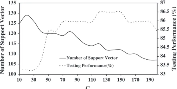
For SVM, the design value ofCanddhas been determined by trail and error approach.Fig. 1shows the fluctuation of testing performance and number for support vector with C. From Fig. 1, it is clear that the number of support vectors is decreas-ing with an increase inC. For the best SVM model, the less number of support vector as well as high testing performance (%) is desirable. SVM produces best testing performance (%) and lowest number of support vector forC= 130 andd= 4. The design value of C(C= 130) and d(d= 4) produces 96.32% training performance, 86.49% testing performance and 112 support vectors. The developed SVM gives the follow-ing equation (by puttfollow-ing K(xi, x) = {(xi.x) + 1}
d , d= 4,
b= 0 and l= 435 in Eq. (4)) for prediction of liquefaction susceptibility of soil. y¼sign X 435 i¼1 aiyifðxixÞ þ1g 4 ! ð16Þ Fig. 2shows the value ofai.
The design value ofcandrhas been determined by trail and error approach in the LSSVM model. Fig. 3 shows the variation in testing performance (%) with c. It is observed fromFig. 3that the developed LSSVM gives best performance at c= 180 and r= 10. The developed LSSVM produces 97.24% training performance and 85.41% testing perfor-mance. The following equation (by putting
Kðxi;xÞ ¼exp ð
xixÞTðxixÞ
2r2
n o
, r= 10, l= 435, and
b= 1.320 in Eq.(8)) has been presented from the developed LSSVM. y¼sign X 435 i¼1 aiyiexp ðxixÞ Tð xixÞ 200 ( ) þ1:320 ! ð17Þ The values ofahave been depicted inFig. 4.
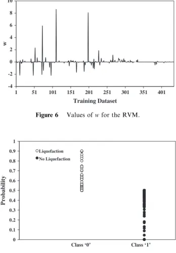
For RVM, the design value ofr has been determined by trail and error approach.Fig. 5illustrates the variation in test-ing performance (%) and number of relevance vector withr. It can be seen fromFig. 5that the testing performance (%) and number of relevance vector increase with an increaser.Fig. 5 also shows that the developed RVM gives best performance at r= 0.06 and number of relevance vector = 265. The devel-oped RVM produces 86.44% training performance and 74.59% testing performance. The developed RVM gives the following equation for prediction of liquefaction susceptibility of soil. 100 105 110 115 120 125 130 135 10 30 50 70 90 110 130 150 170 190 C
Number of Support Vector 83
83.5 84 84.5 85 85.5 86 86.5 87 Testin g Performance (% )
Number of Support Vector Testing Performance(%)
Figure 1 Variation in testing performance (%) and number of
y¼X 435 i¼1 wiexp ðxixÞ T ðxixÞ 0:0072 ( ) ð18Þ Fig. 6shows the value ofw.
The developed RVM gives the probabilistic output.Fig. 7 depicts the probability of training and testing dataset. It is ob-served fromFig. 7that the liquefiable soil fell within the 0.5–1 probability range and most non-liquefiable soil fell within the 0–0.5 range. Thus, the RVM probabilistic output can be used to determine the liquefaction susceptibility of soil. If the out-put is less than 0.5, the probability of liquefaction is decreased. If the output is more than 0.5, the probability of liquefaction is increased.
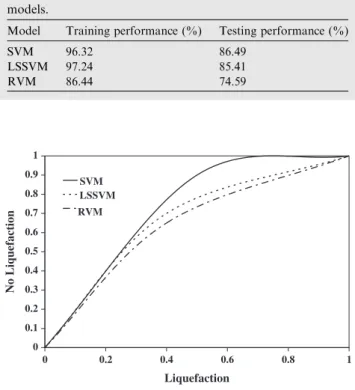
A comparative study has been carried out between the developed SVM, LSSVM and RVM models. Table 1 shows the comparison. The developed SVM and LSSVM outperform the RVM. The performance of the SVM and LSSVM is com-parable. Receiver Operating Characteristics (ROC) has been developed for the SVM, LSSVM and RVM models. Fig. 8 shows the ROC curves. The area under ROC curve is maxi-mum for the SVM. The developed RVM gives the minimaxi-mum area under ROC curve. Therefore, the performance of SVM is best. The developed SVM and RVM use 112 and 265 train-ing dataset for final model respectively. So, the SVM and RVM produce sparse solution. Whereas, the developed LSSVM model uses all training dataset for final prediction. Therefore, it does not produce any sparse solution. The
0 50 100 150 200 250 300 0.01 0.02 0.03 0.04 0.05 0.06
Number of Relevance Vector 40
45 50 55 60 65 70 75 80 Testing Performance (%)
Number of Relevance Vector Testing Performance(%)
σ
Figure 5 Variation in testing performance (%) and number of
relevance vector withr.
-4 -2 0 2 4 6 8 10 1 51 101 151 201 251 301 351 401 Training Dataset w
Figure 6 Values ofwfor the RVM.
0 0.1 0.2 0.3 0.4 0.5 0.6 0.7 0.8 0.9 1 Probability Liquefaction No Liquefaction Class ‘0’ Class ‘1’
Figure 7 Probability of the training and testing dataset from the RVM. -100 -50 0 50 100 150 200 250 300 350 1 51 101 151 201 251 301 351 401 Training Dataset α
Figure 4 Values ofafor the LSSVM.
-10 10 30 50 70 90 110 130 150 170 1 51 101 151 201 251 301 351 401 Training Dataset α
Figure 2 Values ofafor the SVM model.
81 81.5 82 82.5 83 83.5 84 84.5 85 85.5 86 10 30 50 70 90 110 130 150 170 190 Testing Performance (%) γ
developed SVM and LSSVM uses two tuning parameters (For SVM:Candd; For LSSVM:candr). Whereas, there is only one tuning parameter for the RVM model.
6. Conclusion
This article has described SVM, LSSVM and RVM for predic-tion of liquefacpredic-tion susceptibility of soil. 620 data have been utilized to develop the SVM, LSSVM and RVM models. The performance of the SVM and LSSVM is better than that of the RVM. The developed equations can be used by the users for determination of liquefaction susceptibility of soil. The developed SVM and LSSVM produce almost same perfor-mance. The obtained probability from the RVM can be used to determine uncertainty. In summary, it can be concluded that SVM, LSSVM and RVM can be used for solving different problems in engineering.
References
[1] Zadeh Iizuka LA. Fuzzy logic and soft computing Issues, contentions and perspectives in 3rd Int Conf Neural Nets and Soft Computing Fuzzy Logic, Japan, 1994, p. 1–2.
[2]Yuan H, McGinley JA, Schultz PJ, Anderson CJ, Lu C. Short-range precipitation forecasts from time-lagged multimodel ensem-bles during the HMT-west-2006 campaign. J Hydrometeorol 2008;9:477–91.
[3]Toth E. Classification of hydro-meteorological conditions and multiple artificial neural networks for stream flow forecasting. Hydrol Earth Syst Sci 2009:1555–66.
[4]Matas D, Shao M, Biddiscombe Q, Meah MF, Chrystyn S, Usmani H. OS Predicting the clinical effect of a short acting
bronchodilator in individual patients using artificial neural networks. Eur J Pharma Sci 2010;41:707–15.
[5]Yuan CF, Wang WL, Chen Y. An integrated RS and ANN design method for product agile customization. Key Eng Mater 2011;458:212–7.
[6]Santos NI, Said AM, James DE, Venkatesh NH. Modeling solar still production using local weather data and artificial neural networks. Renew Energy 2012:71–9.
[7]Park D, Rilett LR. Forecasting freeway link ravel times with a multi-layer feed forward neural network. Comput Aided Civil Infra Struct Eng 1999:358–67.
[8] Kecman V. Learning and soft computing: support vector machines, neural networks, fuzzy logic models. Cambridge, Massachusetts, London, England, 2011.
[9]Gandomi AH, Alavi AH. Multi-stage genetic programming: a new strategy to nonlinear system modeling. Information sciences, vol. 181. Elsevier; 2011. p. 5227–39 (23).
[10]Gandomi AH, Alavi AH. A new multi-gene genetic programming approach to nonlinear system modeling. Part II: geotechnical and earthquake engineering problems. Neural computing and appli-cations, vol. 21. Springer; 2012. p. 189–201 (1).
[11]Gandomi AH, Alavi AH. Hybridizing genetic programming with orthogonal least squares for modeling of soil liquefaction. Int J Earthquake Eng Hazard Mitigation, Praise Worthy Prize 2013;1(1):1–8.
[12]Alavi AH, Gandomi AH. Energy-based models for assessment of soil liquefaction. Geosci Front 2012;3(4):541–55.
[13]Gandomi AH, Fridline MM, Roke DA. Decision tree approach for soil liquefaction assessment. Hindawi: The Scientific World Journal Press; 2013.
[14]Hanna AM, Ural D, Saygili G. Neural network model for liquefaction potential in soil deposits using Turkey and Taiwan earthquake data. Soil Dynamics Earthquake Eng 2007;27:521–40. [15]Vapnik V. The nature of statistical learning theory. New York:
Springer; 1995.
[16] Liu Y, Gan Z, Sun Y. Static hand gesture recognition and its application based on Support Vector Machines. Proc 9th ACIS Int Conf. Software Engineering, Artificial Intelligence, Network-ing and Parallel/Distributed ComputNetwork-ing, SNPD and 2nd Int Workshop on Advanced Internet Technology and Applications, 4617424 (2008) p. 517–521.
[17]Yazdi HS, Effati AS, Saberi Z. Recurrent neural network-based method for training probabilistic support vector machine. Int J Signal Imag Syst Eng 2009;2:57–65.
[18]Sonavane S, Chakrabarti P. Prediction of active site cleft using
support vector machines. J Chem Inform Modeling
2010;50:2266–73.
[19]Suetani H, Ideta AM, Morimoto J. Nonlinear structure of escape-times to falls for a passive dynamic walker on an irregular slope: anomaly detection using multi-class support vector machine and latent state extraction by canonical correlation analysis. IEEE Int Conf Intell Robots Syst 2011;604843:2715–22.
[20]Kim KJ, Ahn H. A corporate credit rating model using multi-class support vector machines with an ordinal pairwise partitioning approach. Comput Oper Res 2012;39:1800–11.
[21]Suykens J, Vandewalle J. Least squares support vector machine classifiers. Neural Process Lett 1999;9:293–300.
[22] Zhao H, Song C, Zhao H, Zhang S. License plate recognition system based on morphology and LS-SVM, IEEE International Conference on Granular Computing, GRC, 2008, p. 826–829. [23] Xu Y, Deng C, Wu J. Least squares support vector machines for
performance degradation modeling of CNC equipments, CyberC – Int Conference on Cyber-Enabled Distributed Computing and Knowledge Discovery, 2009, p. 201–206.
[24]Ding W, Liang D. Least square support vector machine network-based modeling for switched reluctance starter/generator. Int J Appl Electromag Mech 2010;33:403–41.
Table 1 Comparison between SVM, LSSVM and RVM
models.
Model Training performance (%) Testing performance (%)
SVM 96.32 86.49 LSSVM 97.24 85.41 RVM 86.44 74.59 0 0.1 0.2 0.3 0.4 0.5 0.6 0.7 0.8 0.9 1 0 0.2 0.4 0.6 0.8 1 Liquefaction No Liquefaction SVM LSSVM RVM
Figure 8 ROC curves of the developed SVM, LSSVM and RVM
[25]Siuly S, Li Y, Wen P. Clustering technique-based least square support vector machine for EEG signal classification. Comput Methods Programs Biomed 2011:358–72.
[26]Luts J, Molenberghs G, Verbeke G, Van Huffel S, Suykens JAK. A mixed effects least squares support vector machine model for classification of longitudinal data. Comput Stat Data Anal 2012:611–28.
[27]Tipping ME. The relevance vector machine in advances. In: Solla SA, Leen TK, Muller KR, editors. Neural information processing systems. Cambridge MA: MIT Press; 2000. p. 652–8.
[28] Tipping ME, Faul A. Fast marginal likelihood maximisation for sparse Bayesian models, In: Proceedings of the ninth international workshop on artificial intelligence and statistics, Citeseer, 2003. [29]Widodo A, Yang BS, Kim EY, Tan ACC, Mathew J. Fault
diagnosis of low speed bearing based on acoustic emission signal and multi-class relevance vector machine. Nondestruct Testing Eval 2009:313–28.
[30]Liying W, Zhao W. Forecasting groundwater level based on relevance vector machine. Adv Mater Res 2010:43–7.
[31]Bao Y, Zhang W. A hopfield relevance vector machine algorithm for stock market prediction. J Comput Inform Syst 2011;7:5227–34.
[32]Tsujinishi D, Fuzzy SA. Least squares support vector machines for multi-class problems. Neural Networks Field 2003:785–92.
[33] Liu F, Song H, Zhou QJ. Time series regression based on relevance vector learning mechanism, Int Conference on Wireless Communications, Networking and Mobile Computing, WICOM. 4680839 (2008).
Pijush Samui is a professor at Centre for Disaster Mitigation and Management in VIT University, Vellore, India. He obtained his B.E. at Bengal Engineering and Science Uni-versity; M.Sc. at Indian Institute of Science; Ph.D. at Indian Institute of Science. He worked as a postdoctoral fellow at University of Pittsburgh (USA) and Tampere University of Technology (Finland). He is the recipient of CIMO fellowship from Finland. Dr. Samui worked as a guest editor in ‘‘Disaster Advances’’ journal. He also serves as an editorial board member in several international journals. Dr. Samui is editor of International Journal of Geomatics and Geosciences. He is the reviewer of several journal papers. Dr. Samui is a Fellow of the International Congress of Disaster Management and Earth Science India. He is the recipient of Shamsher Prakash Research Award for the year of 2011.