A note on the relevance of prudence in precautionary saving.
Luigi Ventura
Department of Economics, University of Rome
Abstract
The aim of this note is to suggest that prudence, i.e. convexity of marginal utility, can only explain a small share of precautionary savings, which we may define as savings generated by variance in income. Therefore, if we are willing to admit that precautionary savings
constitute a sizable share of total savings, other factors should be called for. We present a few examples showing that risk aversion might constitute one such factor.
Very helpful comments and stimulating suggestions by Ian Walker are gratefully acknowledged. All remaining errors are my own responsability.
Citation: Ventura, Luigi, (2007) "A note on the relevance of prudence in precautionary saving.." Economics Bulletin, Vol. 4, No. 23 pp. 1-11
Submitted: May 30, 2007. Accepted: June 17, 2007.
A note on the relevance of prudence in precautionary saving.
Luigi Ventura1∗ May 2007
Abstract
The aim of this note is to suggest that prudence, i.e. convexity of marginal utility, can only explain a small share of precautionary savings, which we may define as savings generated by variance in income. Therefore, if we are willing to admit that precautionary savings constitute a sizable share of total savings, other factors should be called for. We present a few examples showing that risk aversion might constitute one such factor.
I. Introduction
The extent of precautionary saving, as a percentage of total savings, has been the object of some theoretical and empirical research, ever since Leland (1968) showed the conditions required for variance in income to stimulate savings.
Leland (1968) showed that an additional requirement was needed, over and above risk aversion, for savings to respond to increasing fluctuations of income around an expected future value, and this was convex marginal utility, or '''( )>0
w
U .
Kimball (1990) named this characteristic of utility functions “prudence”, and defined measures of absolute prudence and relative prudence as ( ) '''( )/ ''( )
w U w U w =− η and, respectively, )( ) '''( )/ ''( w U w wU w =−
ρ , in a way which closely mimicked Pratt (1964)
and Arrow (1965) definitions of absolute and relative risk aversion.
Nevertheless, it seems fair to admit that no consensus has been reached as to the relevance of the precautionary motive for saving.
Estimates of precautionary savings do not abound in the literature, and this is even more the case for estimates of prudence. Merrigan and Normandin (1996), Eisenhauer (2000), and Eisenhauer and Ventura (2003) proposed some estimates of relative prudence, ranging from less than 1 to about 2 for a British sample, between 1.5 and 5.1 for an American sample, and somewhat higher values for an Italian sample. Considering that empirical values of relative prudence seem to be between 3 and 4, numerical simulations by Skinner (1988), Zeldes (1989), Caballero (1991), Deaton (1992), Carroll and Samwick (1998), and Irvine and Wang (2001) suggested that substantial amounts of precautionary saving might be obtained, ranging from 20 to 60 percent of all saving. Actual estimates of precautionary savings seem to be smaller, or at least no larger, than these estimates. Estimates of actual precautionary saving range from almost insignificant figures (as in the works by Skinner (1988), Kuehlwein (1991), Grossberg (1991), Guiso, Jappelli, and Terlizzese (1992), Starr-McCluer (1996), Parker (1999),
1 Dipartimento di Scienze Economiche, Università di Roma “La Sapienza”.
Kazarosian (1997), Alessi and Kapteyn (2001), and Hochguertel (2003)) to suggestions that precautionary savings might represent percentages from around 20% to 60% of total savings (as was the case in the contributions by Dardanoni (1991), Lusardi (1997), Eisenhauer and Ventura (2005)).
The main aim of this paper is to show that prudence can only play a limited role in generating precautionary savings, i.e. savings related to increasing variance in income, and that other factors, such as risk aversion, should also be invoked. We show that this is true, in particular, when we allow saving in risky assets.
The rest of the paper is organized as follows: section II sets the problem of prudence and precautionary saving in a very basic analytical set-up, to provide a simple discussion of the mechanisms at work. Section III discusses the empirical relevance of prudence in determining saving; section IV contains a few examples pointing at the role of risk aversion in generating precautionary savings, and section V concludes, suggesting avenues for further research.
II. A closer look at prudence and precautionary savings
To focus on the essential features of the issue, consider a very simple optimization problem in which an individual, endowed with utility function U(y), consumes in two periods (date 0 and date 1), and faces uncertainty at date 1, in the form of a mean preserving spread ε~ over two possible states of the world. This agent is endowed with income yat date 0 and at date 1 (in expected terms). The two states of the world at date
1 have equal probabilities (without loss of generality). We use a mean preserving spread for simplicity, as we do not want to change the expected income in the second period, which would then provide the agent with an additional, intertemporal, motivation to save. Also for simplicity, we suppose that the rate of time preference equals the rate of return on savings to eliminate impatience as an explanation of savings.
Our agent is allowed to save at date 0, to transfer purchasing power from date 0 to date 1. His problem will therefore be that of choosing s to maximize the expression:
) ( 2 1 ) ( 2 1 ) (y s U y s U y s U − + −σ + + +σ + (1)
The first order condition of the problem can be stated as:
) ( ' 2 1 ) ( ' 2 1 ) ( ' y s U y s U y s U − = −σ + + +σ + (2)
In other words, the marginal utility of present consumption has to be equal, at the optimal solution, to the expected value of the marginal utility of future consumption. Now, if marginal utility is convex, it can be easily shown (see Figure 1 below) that randomness in future income raises expected marginal utility above its level at a certain income, and stimulates saving (all points on the chord represent a particular convex
combination of marginal utility evaluated at the two possible income levels, and thus represent expected marginal utility at date1).
In fact, ceteris paribus, when marginal utility is convex, expected marginal utility of consumption is higher than marginal utility evaluated at the expected value of consumption in the absence of any saving. In other words, when income is affected by a mean preserving spread, saving must rise in order to preserve equality between marginal utility of today’s consumption and expected marginal utility of future consumption. Were marginal utility concave, the opposite would be true.
The increase in saving will be larger the more convex is marginal utility (the larger is prudence, which can be taken as a measure of the gaussian curvature of marginal utility), and the more dispersed is income. Conversely, for very small risks or very small curvatures, saving will hardly depend on prudence.
In passing, we may also notice that in the more general case where the number of states of nature (and corresponding income points) is larger than two, the expected marginal utility of income would always lie below the expected marginal utility of income obtained by concentrating all the probability on the two extreme outcomes. By restraining ourselves to the latter case, therefore, we adopt a very conservative stance (with respect to theory), i.e. one which is likely to overestimate the role of prudence in determining precautionary saving.
Figure 1 Convex marginal utility and precautionary saving
III. Is prudence really crucial in determining precautionary saving?
In view of the previous considerations, an interesting question can immediately be asked: to what extent can convexity of marginal utility, or prudence, be considered responsible of “precautionary” saving, i.e. saving related to income uncertainty? This is largely an empirical question, and will be dealt with in an essentially empirical manner.
To this purpose, let us suppose the instantaneous utility function of our agent belongs to a CRRA family, and has the form:
γ γ − = − 1 ) ( 1 c c u ,
where γ is the coefficient of relative risk aversion. It can be easily shown that for this family of utility functions the coefficient of relative prudence is positive, and equal to
1 +
γ . Notice, however, that any affine transformation of the proposed utility function would lead to exactly the same results, in terms of the results shown below.
By using this instantaneous utility function the overall utility index, defined over consumption at the two dates (0 and 1) and states of the world (α andβ) can be written as: γ γ γ γ β γ α γ β α = − + − + − − − − 1 2 1 1 2 1 1 ) , , ( 1 1 1 1 1 0 1 1 0 c c c c c c U ,
where: c0 = −y s c, , .1α = − +y σ s c1β = + +y σ s By solving the optimization problem:
γ σ γ σ γ γ γ γ β α − + + + − + − + − − = − − − 1 ) ( 2 1 1 ) ( 2 1 1 ) ( ) , , ( max 1 1 1 1 1 0 s y s y s y c c c U s (3)
we obtain a saving function s(y,σ,γ) linking saving to initial endowments, random shocks, and relative prudence.
In fact, rather than directly solving equation (3) in s, which may easily become very
cumbersome (depending on the values of γ ), we will resort to numerical algorithms, to solve for s from the first order condition of problem (3), i.e.:
γ γ γ σ − σ − − = − + + + + − ( ) 2 1 ) ( 2 1 ) (y s y s y s (4)
To solve for s we will substitute data extracted from a few waves of the Bank of Italy
Survey of Household Income and Wealth (SHIW) into (4). The SHIW is a survey conducted by the Research Department of the Bank of Italy every two years on a very large sample of families. The data is organized as a rotating panel, containing many interesting variables, both from socio-demographic and economic standpoints. In particular, we will use these data to compute a measure of income, y, and a measure of
income shocks, σ .
Labour economists have long stressed the importance of linking income to various social and demographic factors, such as age, gender, education level, marital status, etc. We therefore develop a measure of unpredictable income risk, instead of simple income variance (or variance of income growth), as a proxy of income risk from such a model of income determination. In other words, we define income risk as that residual of income variability that cannot be explained by socio-demographic factors. This has the
advantage that we define income risk as that variation that is difficult to explain with easily observed variables and so will be difficult, if not impossible, to insure against. Therefore, we pool together all observations of the Bank of Italy surveys from 1991 to 2000, for which we have two consecutive observations on income, and estimate an income profile equation of the type:
it it it it y X u y =β0 +β1 −1+ 'γ + (5)
where yit−1 is income lagged one period, while the vector Xit includes a set of other variables, such as age, gender, education, wealth and a host of dummy variables indicating the professional status, the sector and area of employment, etc. Standard assumptions are made on the disturbance term uit.
The underlying idea is that the systematic part of expression (5) can be predicted by households, so the residuals might be viewed as a measure of uncertainty. It seems likely that this will lead to an overstatement of income uncertainty, as our model will not capture much of the heterogeneity present in the riskiness of household incomes (which, again, is fine for the purposes of our analysis). In particular, it seems likely that households will have better information than is contained in our data so that some of the variance in uit will be known to the household.
As a (rough) measure of income shocks(σ)we chose to consider the mean (4070) and the median (2605) of the absolute value of estimation errors obtained from the income profile regression, on a yearly basis (the values obtained from the estimation have been divided by two, as the frequency of data is bi-annual). As a measure of y we take the
overall average income in the second period, across all the individuals in the pool. The results obtained from the regression are reported in table A1, in the appendix. In table 1, below, we report the optimal values of s, computed from several specifications
of the CRRA utility function (with γ ranging from 1 to 10). The first and third rows in Table 1 contain the computation of saving according to equation (4), while the second and the forth rows contain the ratio of such measures to total savings (5793).
This (rather wide) range for the parameterγ was set on the basis of some previous empirical works providing estimates for the coefficient of relative risk aversion for Italian households. More specifically, both in the work by Guiso and Paiella (2001) and in Eisenhauer and Ventura (2003) that coefficient is lower than 10. This is also in accord with some existing empirical evidence concerning prudence, as described in section I.
Table 1. Optimal savings induced by convexity of marginal utility, as a function of relative prudence and risk.
γ 1 2 3 4 5 6 7 8 9 10
σ=2605 55.83 83.25 110.16 136.34 161.96 186.49 209.73 231.89 253.17 273.31 % savings 0.96 1.43 1.90 2.35 2.80 3.22 3.62 4.00 4.37 4.72
σ=4070 135.67 200.75 262.82 321.24 375.72 425.82 471.78 513.62 551.58 585.97 % savings 2.34 3.46 4.54 5.54 6.48 7.35 8.14 8.86 9.52 10.11 Note: Values have been computed on the basis of the following parameters: average yearly income = 16384; average yearly total savings = 5793. All values are expressed in euros.
Inspection of table 1 gives us an idea about the relative importance of prudence in determining precautionary savings. In particular, notice that even with rather large shocks, respectively equal to about 8% and 13% of average income, precautionary savings only amount to relatively small values, and that this is true even with fairly large amounts of prudence.
On a percentage basis, precautionary savings would range between 1 and 5% of total savings in the case of the smaller shocks, and from about 2 to 10% of total savings, in case of larger shocks.
In view of the estimates in the literature, referred to in section II, it seems likely that factors other than convexity of marginal utility should be called for to explain savings. IV. Could risk aversion also play a role?
To address this issue, a few simple examples will suggest that risk aversion has an important role to play in determining precautionary saving. A common (and crucial) feature of all the examples is that agents can always save in risky assets, and possibly in a riskfree asset. Given that in real world economies virtually all assets are, at least to some extent, risky, this assumption does not seem particularly strong.
The first two examples will cover the case in which prudence is zero, yet saving is positive and increasing in income variability in the second period. In the third example risk aversion and prudence will coexist, but we will propose a way to isolate the effect of the former.
Example 1.
Consider an agent living in a two period economy, endowed with preferences represented by the utility function, defined over final consumption,
2
20 )
(c c bc
U = − , with b>0 and such that marginal utility is positive. The
agent has initial endowments of w at time 0 and of w+λk and w−λk,
respectively, in the two states of the second period (using the parameter λ, we can suitably modify the variance of future income), and who can save in a risky asset, y, with payoff rα =−k and rβ =k, respectively, in the two states of the
world in the second period, α and β, occurring with equal probabilities for simplicity. The price of y has been normalized to one (to avoid introducing an
equilibrium model to determine the asset price – for example, we might say there exists a properly defined risk neutral individual, who forces the price of y
Our agent solves therefore the following maximization problem:
[
]
[
2]
2 2 ) ( ) ( 20 5 . 0 ) ( ) ( 20 5 . 0 ) ( ) ( 20 β β α α λ λ λ λ r y k w b r y k w r y k w b r y k w y w b y w Max y + − − + − + + + − + + + − − −Setting w=50, and solving the resulting f.o.c. with respect to y, we obtain the
following expression: y=0.495 0.99+ λ−0.099 b. We easily observe that
saving in y increases in income variance in the second period, and in the utility
parameter b (<0.2, to guarantee positive marginal utility), governing risk
aversion. Clearly, in this example precautionary saving is positive as long as income variance in the second period is positive, and zero otherwise (or negative, if one is willing to admit dissaving in y).
Example 2.
The economy is equal to that of Example 1, except for the fact that our agent is allowed to save in two assets: s, paying 1 in both states of the world, and y,
paying off – k and k, respectively, in states α and .β
The maximization problem will now take the form:
[
]
[
2]
2 2 , ) ( ) ( 20 5 . 0 ) ( ) ( 20 5 . 0 ) ( ) ( 20 β β α α λ λ λ λ r y s k w b r y s k w r y s k w b r y s k w y s w b y s w Max y s + + − − + + − + + + + − + + + + − − − − −Setting w=50, and solving the resulting f.o.c.’s with respect to s and y, we
obtain the following expression for total saving (s+y):
0.249 0.497 0.0497
s+ =y + λ− b which is again increasing in income variance,
and increasing in risk aversion. Once more, precautionary savings is positive whenever income variance in the second period is positive.
These two examples have been worked out using a simple quadratic utility function, which has been criticized for the properties it implies in terms of risk attitudes. It is well known that quadratic risk aversion features increasing absolute risk aversion, which seems to be quite implausible, in the light of empirical and experimental evidence to the contrary. In the last example we will modify our economy to introduce more complex preferences. Prudence will no longer be zero, and this will bring in an additional problem, i.e. that of separating the effects of prudence from those of risk aversion.
As in the last example, two assets are available in the economy, with the following payoff structure: asset s, pays off 1 in both states of the world, and y
pays off – k and 0.8 k, respectively, in states α and .β
The investor has preferences represented by the utility function
. 1 ) ( 1 rc c c U − − = − γ γ
For r =0this utility function corresponds to well known
preferences, of the CRRA type, for which the following relationship holds between the coefficient of relative risk aversion,R(c), and the coefficient of relative prudence,ρ(c): ρ(c)=1+R(c)=1+γ . The parameter rcan therefore
be used to breach the linear relationship between risk aversion and prudence. In fact, it only affects the first derivative of the utility function, which enters the denominator of risk aversion coefficients, without affecting its second and third derivative, which leaves the coefficients of prudence unaffected. The only restriction that we place on ris that it be compatible with positive marginal
utility.
In this example we also constrain the investor to buy positive quantities of s and y (dissaving is not allowed). Our agent has the option of saving in the two assets
and decides the allocation by solving the following problem:
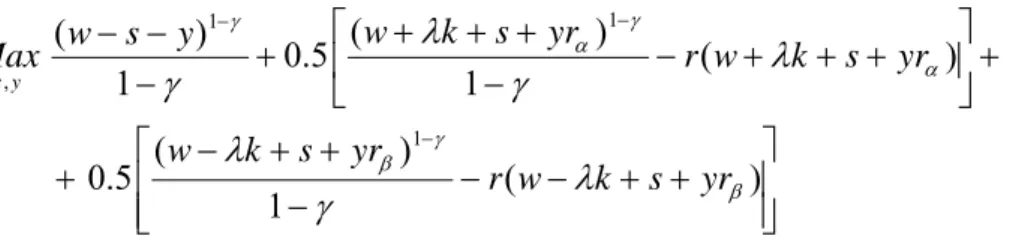
⎥ ⎥ ⎦ ⎤ ⎢ ⎢ ⎣ ⎡ + + − − − + + − + + ⎥ ⎦ ⎤ ⎢ ⎣ ⎡ + + + − − + + + + − − − − − − ) ( 1 ) ( 5 . 0 ) ( 1 ) ( 5 . 0 1 ) ( 1 1 1 , β γ β α γ α γ λ γ λ λ γ λ γ yr s k w r yr s k w yr s k w r yr s k w y s w Max y s
where we have set r =0 for the first period and, for simplicity, the price of both
assets has been normalized to 1. Differentiating with respect to s and y we get the first order conditions:
0 ) ( 5 . 0 ) ( 5 . 0 ) ( − − + + + + + + + + − = − − − − r yr s k w yr s k w y s w γ λ α γ λ β γ and ( ) 0.5 ( ) 0.5 ( ) 0.5 0.5 0 w s y r w k s yr r w k s yr r r r r γ γ α α γ β β α β λ λ − − − − − − + + + + + + + + − − = .
In view of the complexity of first order conditions for generic values of γ we do not have closed form solutions, as in the previous examples, but report in Table 2 below the optimal choices of s and y corresponding to several values ofλ and r.
Notice that an increase in λ will always generate an increase in overall savings and in its components (which is consistent with the idea that more income variability in the second period brings about more savings, both risky and riskless); more importantly, though, we can observe that an increase in risk aversion (higher r) will also increase overall savings, at least for certain ranges
of λand r. As the latter goes up, saving in the riskless assets will go down,
whereas saving in the risky asset will increase, with an ambiguous effect on overall savings. As risk aversion rises over a certain threshold, total savings will also rise, if no short sales of the riskless assets are allowed. We might describe the mechanism at work as follows: as the dispersion of income in the second period increases, the investor buys larger and larger quantities of the risky asset, to insure, and sells the riskless asset to offset the increase in marginal utility at date 0. The motivation to save, highlighted by Leland (1968) and hinging crucially on convexity of marginal utility, may therefore be partially or completely offset by the desire to insure. However, as r goes up, saving in the
riskless asset hits its lower bound (i.e. 0), and there will be no trade off between saving in the two assets. Total saving will unambiguously increase, and this growth will be governed by risk aversion.
V. Conclusions and avenues for future research
In the previous paragraphs the role of prudence, i.e. a parameter measuring the curvature of marginal utility, was investigated in relation to saving induced by income risk. By a simple calibration of the first order condition for utility maximization with actual Italian data, it was shown that even in fairly extreme cases (i.e. rather large income shocks, and large values for relative risk aversion and prudence) the convexity of marginal utility might only account for relatively small percentages of total savings. This suggests, of course, that if one is willing to attribute a large percentage of savings to the riskiness of income, then other factors should also be invoked apart from prudence. One such factor is risk aversion, which drives individual efforts to hedge against unforeseen contingencies, thereby stimulating saving in state contingent (risky) assets.
To stress this point, a few simple examples showed that, as the variance of income in the second period increases, an investor buys larger and larger quantities of an asset with risky returns, to obtain insurance, possibly selling a safe asset to offset the consequent increase in marginal utility at date 0. In this case, the role of prudence in determining saving may be overcome by the desire to insure. Nevertheless total saving, which one might correctly define “precautionary”, since it is originated by variance in income, turns out to be increasing in the latter, but might be governed by risk aversion, rather than prudence. Importantly, the first two examples show that even when prudence is zero, may we find precautionary savings, when both income risk and risk aversion are positive. λ r 0.00 0.01 0.02 0.03 0.04 0.05 2 2.22 1.32 1.61 1.89 2.17 2.44 3 3.33 2.45 2.72 2.99 3.26 3.52 4 4.44 3.57 3.83 4.09 4.35 4.59 5 5.55 4.70 4.95 5.19 5.44 5.67
The interplay between risk aversion and prudence seems therefore to constitute an interesting topic to explore in further work, both from a theoretical and an empirical point of view. In particular, from a more theoretical point of view it would be interesting to find out conditions under which the effect of risk aversion predominates over that of prudence, or vice versa; from a more empirical standpoint it could as well be interesting to analyze the behaviour of individuals affected by large (unpredictable) uncertainty, both in terms of amounts saved, and in terms of instruments used for saving.
VI. References
Alessi, Rob and Arie Kapteyn. (2001). “Savings and Pensions in the Netherlands”
Research in Economics, 55(1), 61-82.
Carroll, Christopher D. and Andrew A. Samwick. (1998). “How Important Is Precautionary Saving?” Review of Economics and Statistics, 80(3), 410-419.
Dardanoni, Valentino. (1991). “Precautionary Savings under Income Uncertainty: A Cross-Sectional Analysis” Applied Economics, 23(1B), 153-160.
Eisenhauer, Joseph G. (2000). “Estimating Prudence” Eastern Economic Journal, 26(4),
379-392.
Eisenhauer, Joseph G. and Luigi Ventura. (2003). “Survey Measures of Risk Aversion and Prudence” Applied Economics, 35(13), 1477-1484.
Eisenhauer, Joseph G. and Luigi Ventura. (2005). “The Relevance of Precautionary Saving ” German Economic Review, 6, 1465-1485.
Grossberg, Adam. (1991). “Personal Saving under Income Uncertainty: A Test of the Intertemporal Substitution Hypothesis” Eastern Economic Journal, 17(2), 203-210.
Guiso, Luigi, Tullio Jappelli, and Daniele Terlizzese. (1992). “Earnings Uncertainty and Precautionary Saving” Journal of Monetary Economics, 30(2), 307-337.
Hochguertel, Stefan. (2003). “Precautionary Motives and Portfolio Decisions” Journal of Applied Econometrics, 18(1), 61-77.
Irvine, Ian and Susheng Wang. (2001). “Saving Behavior and Wealth Accumulation in a Pure Lifecycle Model with Income Uncertainty” European Economic Review, 45(2),
233-258.
Kazarosian, Mark. (1997). “Precautionary Savings—A Panel Study” Review of
Economics and Statistics, 79(2), 241-247.
Kimball, Miles S. (1990). “Precautionary Saving in the Small and in the Large”
Econometrica, 58(1), 53-73.
Kuehlwein, Michael. (1991). “A Test for the Presence of Precautionary Saving”
Economics Letters, 37(4), 471-475.
Leland, Hayne E. (1968). “Saving and Uncertainty: The Precautionary Demand for Saving” Quarterly Journal of Economics, 82(3), 465-473.
Appendix
This appendix contains the result of the estimation of an income profile equation, described in section (III). Data come from the Bank of Italy Survey on Household Income and Wealth, pooling observations from 1991 to 2000.
Table A1. Income profile estimation
Variable Coefficient P - Value
1 − t Y 0.43 0.00 D91 -1486.23 0.00 D93 -481.49 0.01 DS -1281.69 0.00 WEALTH 0.01 0.00 EDUCATION 2022.31 0.00 AGE 40.09 0.00 DQ1 -1096.55 0.02 DQ2 -1835.03 0.00 DQ5 -1115.99 0.00 DS1 1633.68 0.01 DS2 3218.93 0.00 DS3 2093.03 0.00 DS4 2188.09 0.00 DS5 4032.00 0.00 DS6 8198.27 0.00 DS7 5253.29 0.00 DS8 3315.08 0.00 UNEMPLOYMENT 409.37 0.00 GENDER (f) -1234.80 0.00 R-squared 0.56
Table A1 contains the results of an OLS estimation of equation (5). This equation yields income at time t (Yt) as a function of income (measured in € per year) at time t – 1 and a set of other control variables, including age (in years), gender (1=female?), years of education, wealth (in euros) and a set of dummy variables indicating the professional status (DQ1, DQ2, and DQ5 denote, respectively: a blue collar worker, an office worker or school teacher, and others who are not employed, and the omitted category is junior managers and cadres), employment sector (indicating, respectively: agriculture, manufacturing, building and construction, wholesale and retail trade, transport and communication, credit and insurance, real estate and renting services, general government, and the omitted categories are domestic and other private services and extraterritorial organizations), and time dummies (D91 and D93 corresponding to 1991 and 1993 observations, respectively, whereas dummies for 1995, 1998 and 2000 have been omitted).
Variables are expressed in levels, as a log-level version of the same equation led to somewhat worse results. Variables with non significant coefficients have been removed from the estimated equation.