Michigan
University ofResearch
Retirement
Center
Working Paper
WP 2010-238
M R
R C
Project #: UM10-14
Intergenerational Transfers in the Health and
Retirement Study Data
Intergenerational Transfers in the Health and Retirement Study
Data
John Laitner
University of MichiganAmanda Sonnega
University of MichiganNovember 2010
Michigan Retirement Research Center
University of Michigan
P.O. Box 1248
Ann Arbor, MI 48104
http://www.mrrc.isr.umich.edu/
(734) 615-0422
AcknowledgementsThis work was supported by a grant from the Social Security Administration through the Michigan Retirement Research Center (Grant # 10-M-98362-5-01). The findings and conclusions expressed are solely those of the author and do not represent the views of the Social Security Administration, any agency of the Federal government, or the Michigan Retirement Research Center.
Regents of the University of Michigan
Julia Donovan Darrow, Ann Arbor; Laurence B. Deitch, Bingham Farms; Denise Ilitch, Bingham Farms; Olivia P. Maynard, Goodrich; Andrea Fischer Newman, Ann Arbor; Andrew C. Richner, Grosse Pointe Park; S. Martin Taylor, Gross Pointe Farms; Katherine E. White, Ann Arbor; Mary Sue Coleman, ex officio
Intergenerational Transfers in the Health and Retirement Study
Data
Abstract
Many economic analyses of public policy issues are based upon the life-cycle model of household behavior. The usual formulation omits private intergenerational transfers. This paper considers the possibility of a more sophisticated formulation that includes the latter.
We examine 1992-2008 HRS data on inheritances and inter vivos gifts. We uncover an underreporting problem in the data: a household’s financial respondent often seems to understate transfers from his/her in-laws. Nevertheless, other aspects of the data seem very useful. About 30-40 percent of households eventually inherit. Inheritances seem to reflect a mixture of intentional and accidental bequests, with the latter twice as prevalent.
Authors’ Acknowledgements
This work was supported by a grant from the Social Security Administration through the Michigan Retirement Research Center (Grant # 10-M-98362-5-01). John Laitner also thanks NIA, grant PO1-AG029409, for support.
Intergenerational Transfers in the Health and Retirement Study Data John Laitner and Amanda Sonnega
November 4, 2010
Much economic analysis of the Social Security system is based on the life-cycle model (Modigliani [1986], Auerbach and Kotlikoff [1987]). Although this framework can encom-pass many phenomena of interest, its scope is limited, as its name implies, to singles or couples whose attention focuses on their own well-being, over their own life span. In partic-ular, the model does not include concerns of households in one generation for predecessors or descendants in their family line, manifestations of such sentiments in the form of in-tentional intergenerational transfers between parents and grown children, or nonmarket exchanges of property and services between related households. The purpose of this paper is to utilize data from the Health and Retirement Study (HRS) on private, intergenera-tional transfers between parents and children (the latter being participants in the HRS) to assess the magnitude of such transfers and the possible motives behind them. Aside from the general usefulness of data dissemination, we believe that this work will be of long-term interest to the Social Security Administration because (a) so much economic analysis of Social Security-related issues rests on the life-cycle model that efforts to improve its predictive power are important; and, (b) documenting the prevalence and motivation for intergenerational transfers – a potentially underspecified component of householdfinances – will help policymakers who need to understand the well-being of different households and the distributional impacts of public transfer programs.
Private-sector intergenerational transfers are potentially significant. For example, es-tate creation may be an important motive for saving, especially among high-income house-holds; intergenerational transfers may augment, and sustain, inequality between family lines; and, bequests (and gifts) may connect generations in ways that provide insurance. This paper seeks to study the intergenerational-transfer data resources of the Health and Retirement Study (HRS) data. We are particularly interested in transfers to married cou-ples, the modal recipient-household type. This paper constructs a simple model of the distribution of inheritances and uses it to analyze and assess the HRS data. Our goals are to gain an understanding of underlying parental behavior and of the HRS data’s strengths and weaknesses, including appropriate avenues for more detailed analysis in the future.
The HRS provides a large sample, an extensive set of questions on transfers, and a very rich set of covariates. The HRS utilizes a combination of retrospective questions on past transfers and wave-to-wave questions on receipts over current two-year intervals. In contrast to many surveys, the HRS asks households about the sources of their major gifts and inheritances. The latter detailed information provides the foundation of this paper’s analysis.
As is common, the HRS relies upon a single respondent, the “financial respondent,” to provide household data for a couple. Using our model in concert with findings from the existing literature about the equality of division of parental estates, we conclude that HRS
financial respondents tend to report transfers from their parents-in-law. The under-reporting seems severe, and we propose utilizing financial respondent reports of transfers
from their own side of the family only. We argue that this can raise estimated average transfer amounts 30-100 percent. (And, it may have implications for other data sources.)
We also show that conditional data on spousal inheritances – conditional on a recorded positive amount – may be valuable despite shortcomings of the unconditional
figures. A strand of the existing literature distinguishes intentional from accidental inter-generational transfers, and we suggest that HRS data provides some support for a mixture of the two – and particular support for the accidental model.
We have data on inter vivos gifts (from the Wealth Section of the HRS) as well as inheritances. We show that it tends to accent gifts at relatively advanced ages. The prevalence and magnitude of these transfers seems important. However, we argue that the survey’s methodology may inadvertently lead to a neglect of early-in-life gifts. Analysis suggests that the distribution of gifts resembles that of inheritances. On the one hand, this is as one would expect: there is no reason that reporting problems would be
con-fined to inheritances. On the other hand, it is somewhat puzzling that gifts, which must nearly always be intentional, would tend to resemble inheritances, which may be mainly accidental.
The organization of this paper is as follows. Section 1 reviews the existing literature. Section 2 summarizes characteristics of the HRS intergenerational transfer data. Section 3 examines agent reporting errors. Section 4 considers evidence in the data for intentional bequests and assortative mating. Section 5 briefly examines HRS data on inter vivosgifts. Section 6 attempts to assess what we can say about the relative frequency of intentional versus accidental private intergenerational transfers. Section 7 concludes.
1. Existing Literature
This section briefly reviews the theoretical and empirical literatures on private inter-generational transfers.
This paper focuses on two major models of private intergenerational transfers. The
first we might call the “intentional-bequest model.” In the most widely studied variant (Becker [1974], Barro [1974]), the “altruistic model,” parents care about their own lifetime utility, say, u(cP), with cp = parent household lifetime consumption, and their grown
chil-dren’s utility, say, in the case of a single child, u(cc), with cc = child household lifetime consumption. Then the parent household’s total utility might beu(cP) +ω·u(cc), whereω
is the weight the parents attach to the child’s lifetime utility relative to their own. Presum-ably ω ∈[0, 1]. The higher ω is, the stronger the parents’ altruism. This model has been used to study saving (Kotlikoff and Summers [1981], Kotlikoff [1988], Modigliani [1988], Laitner [1992]), fiscal policy (Barro [1974]), human capital accumulation (Becker [1980], Loury [1981]), and inequality (Laitner [2002]).
One important characteristic of altruistic bequests is that they may be narrowly con-centrated. If children earn more than their parents – a frequent occurrence in a progressive economy – and if institutions require that bequests be non-negative, many altruistic be-quests will be zero. Only parents well-off relative to their children will want to make positive transfers. The threshold for a positive bequest will be higher if ω (see above) is lower.
Another large literature studies incomplete annuity markets, which can give rise to “accidental bequests” (e.g., Davies [1981], Abel [1985], Kotlikoff and Spivak [1981], and others). Friedman and Warshawsky [1990], for example, propose a formulation in which parents would like to set aside part of their net worth for a bequest to their children and annuitize the rest for their own use in retirement. Annuity prices tend to be unattractive, however, because of adverse selection (i.e., households most inclined to purchase annuities are those which expect to live an unusually long time). Thus, parental concerns about leaving an estate make them reluctant to participate too extensively in the annuities mar-ket. With incomplete annuitization, a parental estate will vary with time of death: if the parents die young, it will be large; if they live a very long time, it may disappear entirely. Again, accidental bequests need not be pervasive. Social Security is an annuity, as are some pension payouts. If institutions prevent negative bequests, parents who enjoy exceptional longevity may exhaust all of their unannuitized resources and die with a zero bequest.
There have been a number of empirical studies. One strand of literature focuses on heterogeneity of bequests within family lines. The altruistic model would seem to imply that parents should direct larger bequests to their least prosperous children. Yet, evidence suggests that parents actually divide their estates quite equally in a substantial majority of cases (Menchik [1980, 1988], Walker [2005], Wilhem [1996], Kessler and Masson [1989]). A second strand of literature compares private transfers across the parent-child pairs from different family lines. These studies have heavy data requirements. Resulting tests for altruistic behavior depend upon coefficient sign patterns and/or quantitative parameter constraints. Support for the altruistic, intentional-bequest model is mixed. Laitner and Ohlsson [2001] and Laitner and Juster [1996], for instance, find agreement with the sign patterns that the model predicts. However, quantitative parameter constraints often fail by a wide margin (e.g., Altonji et al [1997], Laitner and Ohlsson [2001]). Other evidence seems at variance with the altruistic model as well (e.g., Altonji et al [1992], Hurd [1987]). Family-line transfers can take the form of inter vivos gifts as well as bequests. These seem important in practice (e.g., Gale and Scholz [1994]). Because such transfers seem unambiguously intentional, their existence tends to support the altruistic model. Some empirical evidence suggests that parents may divide their gifts less equally than their bequests (Dunn and Phillips [1997], McGarry and Schoeni [1995], McGarry [1999]). Again, however, data requirements are so severe that many questions remain.
Comparing the behavior of households with and without children, Hurd [1989] finds support for the accidental model. In general, with fewer dramatic implications, the acci-dental model seems harder to defend or dispute than the altruistic specification.
2. HRS Intergenerational Transfer Data
This section examines intergenerational transfer data from wealth sections of the main HRS survey. The HRS began in 1992 with respondents aged 51-61 (though their spouses, of course, could be outside that range). The 1992 HRS survey has an extensive battery of questions, separately asking households about inheritances, trusts, life insurance settle-ments, and gifts received. The questions refer to transfer receipts over the respondent’s
lifetime to date. For each type of transfer, respondents are asked to list the amount, year, and source (i.e., parents, parents in law, siblings, etc.) for the three largest sums.1
Subsequent survey waves (i.e., 1994, 1996, etc.) use an abbreviated sequence of ques-tions, asking about transfers received since the last interview. The questions no longer distinguish ordinary inheritances from transferred trusts. And, after 1992, only for inher-itances are respondents asked the source of the transfer.
This section discusses the general characteristics of the transfer data. A problem emerges regarding the sources of inheritances, and it is the focus of Sections 3-5.
Transfer Data. Table 2.1 presents summary statistics for 1992 HRS. This paper con-centrates on data from the “Net Worth” section of the survey (“Net Worth other than Housing” in 1992, “Net Worth” in 1994, “Assets and Income” in 1996, etc.).
Table 2.1’s top panel presents survey amounts in current dollars. The middle converts all sums to 2005 dollars. The bottom panel accumulates all 2005-dollar sums to 2005 present values, using a real interest rate r = 0.03, i.e., 3%/year.2 Together the two
corrections raise magnitudes by a factor slightly above 4. We can see that a fraction 1584/7702 ≈ 1/5 of 1992 households record the receipt of at least one transfer. Among 1992 HRS households, the average amount received is about $10,000 in the top panel; in 2005 present value terms, it is about $46,000. Limiting attention to households with a positive transfer, the average amount in panel 3 is about $225,000.
In each case, the survey asks whether the respondent has received a given type of transfer, and, if the respondent replies “yes,” the survey asks the amount. If the amount is missing, Table 2.1 records a “censored observation.” A censored observation can have either a 0 or a positive amount. For example, if a household reports 1 or more inheritances yet all its inheritance amounts are missing, its entry for the data of Table 2.1 is 0 but that entry is flagged as “censored.” If, on the other hand, the respondent provides an amount, say, $10,000, for his/her largest inheritance but records a second inheritance without providing its amount, his/her Table 2.1 inheritance would be positive, namely, $10,000, yet the observation would also be flagged as censored. Table 2.1 shows that about 20 percent of households have censored observations. This section devotes no special attention to the latter – in part because the fraction of censored observations seems fairly constant across all subsets of data that we consider.
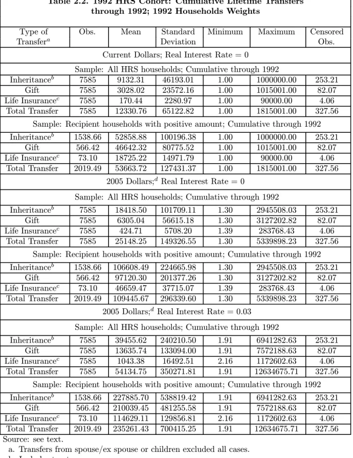
Table 2.2 provides weighted outcomes, using 1992 HRS household weights. Total transfers are roughly 15 percent larger – principally because a higher fraction of the weighted sample has a positive transfer amount. The remainder of this analysis uses weighted data unless otherwise noted.
1 Additional details are that respondents were offered the chance to aggregate transfers
beyond the 3 largest into an “other” category in each of the cases; that gift and insurance settlement amounts were to be $10,000 or more only, though no such restriction was put on inheritances and trusts; and, that we impute missing dates, using the average date for the category in question. The latter imputations affect about 20 percent of the cases within each category.
2 The literature assumes real interest rates of 0.00-0.08. Readers interested in the lowest
Detailed comments about the data are as follows.
Life Insurance. Benefactors can transfer resources by making heirs the beneficiaries of their life insurance policies. In this, as in all categories, we exclude amounts from children and spouses. In the case of insurance settlements, the last group is large. There are 391 life-insurance settlements recorded, but 321 do not pass our criteria. HRS questions after 1992 no longer refer to “life insurance” (rather to “insurance” in general) and, most important, do not ask the beneficiary’s relationship to the heir. Thus, we lack usable data on insurance settlements after 1992. Fortunately, Table 2.1 shows that only 2-3% of 1992 total transfers come from this source.
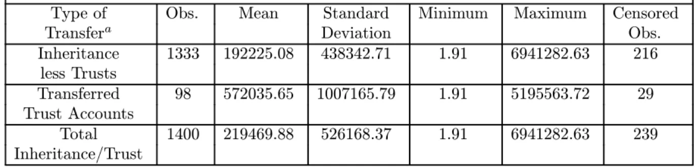
Trusts. The 1992 HRS enables us to measure assets passed in trusts. Table 2.3 provides details. Transfers via trusts are rare, only about 6 percent as frequent as regular inheri-tances. However, they are 3 times as large on average. Thus, they constitute 15-20 percent of total inheritance amounts. HRS waves after 1992 ask respondents for the sum of regular inheritances and transferred trust accounts – and the two cannot be separated.
Inter Vivos Gifts. The meaninter vivosgift in Table 2.1 is almost as large as the mean in-heritance: in the last part of Table 2.1, the mean inheritance (including trusts) is $220,000, while the mean gift is $205,000. Gifts are about one-third as frequent; so, the mean 1992 total transfer is roughly 3 parts inheritance (and/or trust) and 1 part gift. The HRS wealth section in the survey waves 1994 and 1996 stopped asking about gifts – specifi -cally telling respondents not to include them. Beginning in 1998, “gifts” re-emerge in the wealth-section list of questions. However, the frequency gifts reported 1998 and beyond in the wealth section is very low.3
A surprise emerges as we move down Table 2.1: the ratio of the average size of inheritances and gifts is about the same in all three panels. We might expect gifts to occur mainly in the early adulthood of recipients – as parents seek to alleviate children’s liquidity constraints, helping them to make the down payment on their first home, etc. Inheritances, in contrast, presumably flow mainly at the death of the second parent, which tends to occur in the child’s late middle age. Table 2.1, however, contradicts this scenario. As we make price and present value corrections, the ratio of gift to inheritance amounts remains the same. If gifts occurred earlier in life than inheritances, their upward corrections as we move down Table 2.1 would be larger.
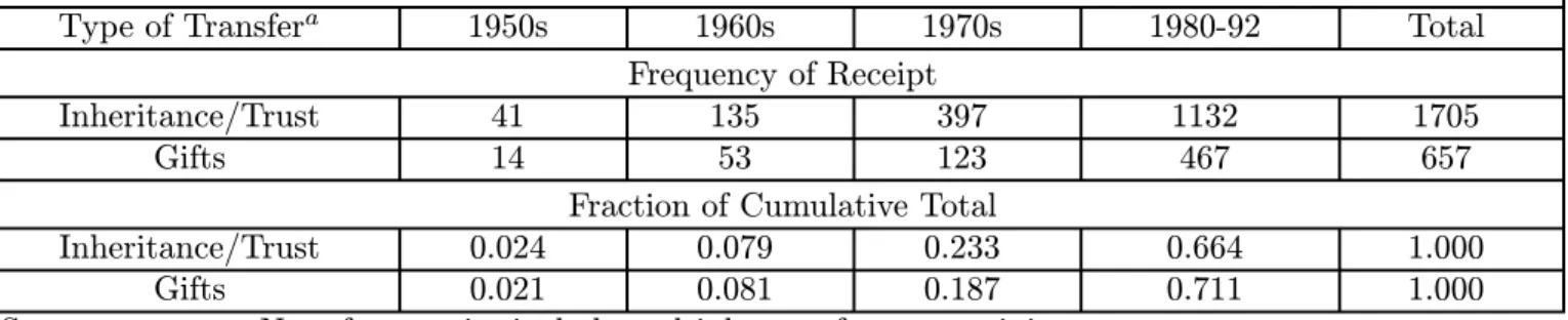
Table 2.4 investigates the latter point in more detail. The table shows that frequencies of inheritance and gift transfer receipt over different decades are very similar for the 1992 HRS cohort.4
We can conjecture various explanations for this outcome – possibly some of the largest gifts are assistance for grandchildren’s higher education; possibly some of the largest transfers that parents make consist of tangible property (e.g., a vacation home) that parents
3 Other sections of the HRS ask about transfers of money and time within the last two
years. Future work will seek to integrate these with the wealth-section data.
4 Notice that recipients may report more than one inheritance, and more than one gift.
Thus, the total numbers of transfers in Table 2.4 need not correspond to the total number of recipient households in Table 2.1.
do not want the responsibility of maintaining in their retirement; or, perhaps some gifts are made, as a tax lawyer would say, “in contemplation of death.”
It also seems possible that many gifts are omitted. The survey asks for major transfers, with major meaning large in the sense of the top panel of Table 2.1. Transfers occurring when a child graduated from school might be small in absolute size – and therefore excluded from reported “gifts” – despite being large in 2005 dollars and present value. For example, $10,000 received in 1982 (the average date for receiving a gift in the survey) is $36,800 in present value by 2005, with 2005 dollars. However, $10,000 received in 1955, would become $261,500 in panel 3 of Table 2.1. Although analysis tends to focus on the bottom panel of Table 2.1, respondents are asked to prioritize their survey time on the basis of the top panel.5
A final surprise is the lack of overlap in gift and inheritance receipts. For example, in the last four rows of Table 2.1 the sum of recipients of inheritances, gifts, and life insurance settlements roughly equals the number of households receiving any transfer at all, indicating that the receiving groups are virtually disjoint. The literature suggests that parents intending to make a bequest might transfer part of the sum early if their children were liquidity constrained. That might lead us to expect that may households that inherit also have gifts – but this is not what Table 2.1 shows.
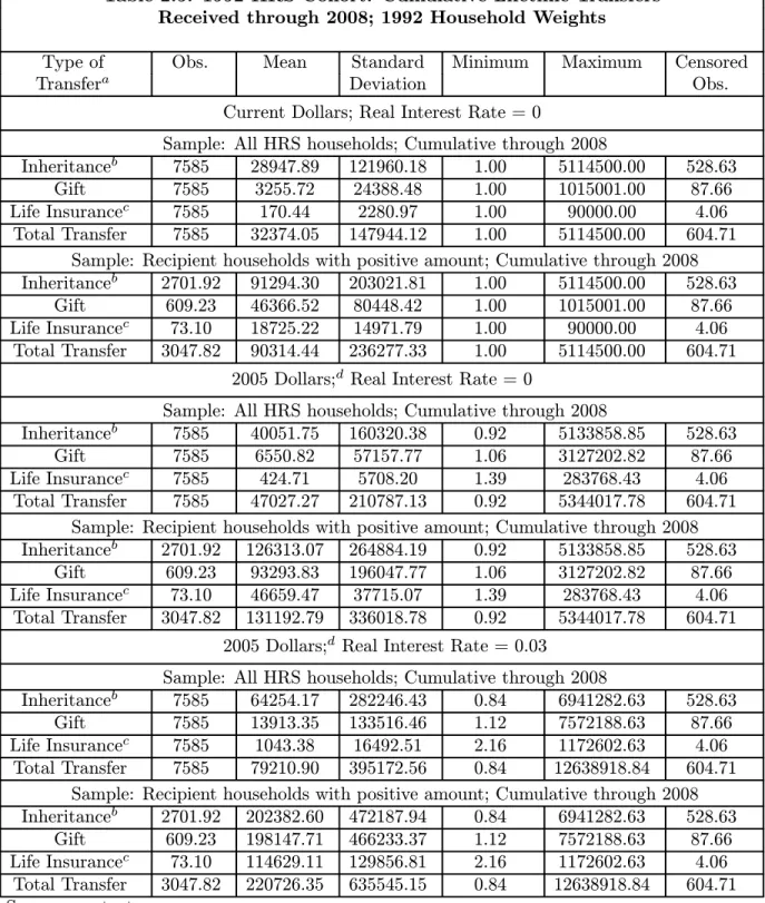
Transfers Through 2008. Table 2.5 accumulates transfers from the 1992 HRS cohort over all survey waves through 2008.
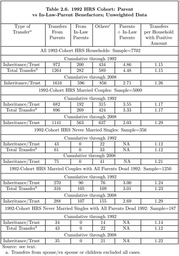
Benefactors. One member of each HRS couple is designated thefinancial respondent, and this individual answers survey questions in the HRS wealth section on behalf of his/her household. On the basis of the existing literature, we expect a couple’s transfer (at least for transfers at death) to be split quite equally among all of its children. The literature provides little evidence that male and female children, for instance, receive different treatment. With this in mind, we expect numbers of transfers from parents and parents-in-law to be roughly equal in the HRS data. Table 2.6, however, does not bear this out.
The top panel of Table 2.6 shows that transfers “from parents” are 3-5 times as prevalent as those “from parents-in-law.” Panels 2 and 4 focus on couples. The inequality of transfers from parents and parents-in-law is somewhat attenuated but still evident – transfers from parents are 2.0-3.5 times as prevalent as those from parents-in-law.
The discrepancy between Table’s 2.6 benefactor ratios and the existing literature is the focus of Section 3.
Section 3: Data Quality
The inequality of parents and parent-in-laws in Table 2.6 leads us to suspect that inheritances from non-financial respondents are understated in the HRS. We now examine
5 Yet another possibility is that respondents sometimes categorize an inheritance – a
transfer from a decedent – as a “gift.” However, we are skeptical that this is an important problem. The 1992 HRS asks about trusts and inheritances; then it asks about gifts. The gift question is: “Excluding inheritances and trusts, have you ever received money or assets totaling $10,000 or more from a relative?” The survey also includes a definition: “[This] could be in the form of support, a gift, or a loan.”
this issue in detail. We investigate what might have gone wrong through a series of hypotheses, examining the evidence for each.
Our initial hypotheses are:
(H1. Misclassification): HRS respondents sometimes name “parents” as their benefactor without going further down the survey questionnaire’s list of options to see that “parents-in-law” is another choice.
(H2. Respondent Fatigue): Although the survey invites respondents to describe many transfers, most respondents only make the effort to record a small number (c.f., Table 2.6). Respondents who choose to mention any transfers at all tend to focus on those with which they have the greatest familiarity, namely, transfers from their side of the family.
Theory. We start with a simple model. The existing empirical literature (see above) suggests that parents divide their estates equally among their children. In particular, male and female children are treated alike, as are married and single children. In the context of our model, these findings can establish what we expect to observe, providing a basis for evaluating the data’s quality.
Begin with two examples. In the first, think of an economy in which parents always have two children, a male and a female. There are 3 types of parents, A, B, and C. The types are equally prevalent. Suppose type A desires to leave a bequest x to each of its children, but types B and C want no bequest at all. SupposeN2 children of each sex choose
to marry, and N1 choose to remain single. Let the marital choice be random. Indexed by
parent types, the support of the distribution of next-generation couples is {AA , AB , AC , BA , BB , BC , CA , CB , CC}.
Suppose mating is random so that all 9 mating patterns are equally prevalent. Let there be N men and N women per cohort. Then
N =N1+N2.
In this framework, the average inheritance per single is
x
3.
For couples, N2/9 are type AA and have inheritance 2·x; 4·N2/9 are AB, AC, BA, or
CA, having inheritance x; and, the remaining 4·N2/9 have inheritance 0. The average
inheritance for next-generation couples is, therefore, 2·x· N29 +x· 4·9N2 N2 = 6 9 ·x = 2 3 ·x .
In other words, the mean inheritance per couple is twice the mean for singles. Intuitively, couples have 2 sets of potential benefactors whereas singles have only 1; hence, couples, as a group, inherit twice as much.
As a second example, change only the mating pattern. Suppose now that mating is rigorously assortative – so that the only couple types in the next generation are
AA, BB, CC.
Given the underlying distribution of parent types, each of the three couple types is equally likely. Singles are unaffected and have the same average inheritance as before. An AA couple inherits 2·x; a BB or CC inherits 0. So, the average inheritance per couples is
1 3 ·2·x+ 2 3 ·0 = 2 3 ·x .
Again, the average inheritance for a couple turns out to be twice the average for a single. A simple model shows that the results above are quite general. Suppose that parent types are indexed with i ∈ {0, 1, ..., I} and that p(i) is the population share of type i. Suppose type i parents bequeath x(i) to each child. Use the indexing convention
x(i) = 0 if i= 0, x(i)>0 if i >0.
Let I N. Provided the marital status “single” emerges randomly, the average inheri-tance per single in the next generation is
m≡3
i
p(i)·x(i). (1)
Couples are slightly more complicated. Nevertheless, we have
Proposition 1: Whatever the nature of mating patterns, the average inheritance per
couple is mc = 2·m.
Proof: Consider the universe of new couples. As a group, the men who marry inherit
N2·
3
i
p(i)·x(i).
The total inheritance of the women who marry is the same. Thus, the average inheritance per couple is mc = N2· i p(i)·x(i) +N2· i p(i)·x(i) N2 = 2·3 i p(i)·x(i) = 2·m .
In fact, the same argument provides more detailed implications:
Corollary 1: Whatever the nature of mating patterns, male spouses, on average, inherit
Proof: Looking at the preceding proof, the average inheritance per male spouse is N2·i p(i)·x(i) N2 =3 i p(i)·x(i) =m .
The same is true for female spouses.
Turn next to the question of who inherits a positive amount. In the case of singles, the number is
N1·
3
i=0
p(i).
Thus, the fraction of singles with a positive inheritance is f, where
f ≡ N1 · i=0 p(i) N1 =3 i=0 p(i). (2)
For couples, we have
Proposition 2: Whatever the nature of mating patterns, the fraction of married
indi-viduals who inherit, fM ar Inds, is 2·f.
Proof: For male spouses, the total number inheriting is N2·i=0 p(i). So, the fraction
inheriting is N2·i=0 p(i) N2 =3 i=0 p(i) =f .
The same argument applies to female spouses. So,
fM ar Inds = 2·f .
Proposition 2 provides a way of evaluating (H1) directly. Its proof, however, also suggests a way of evaluating (H2).
Corollary 2: Whatever the nature of mating patterns, the fraction of male spouses with
positive inheritances is f = i=0 p(i), and the fraction of female spouses, and singles, with positive inheritances is the same.
Proof: See the proof of Proposition 2.
Digressing, note that neither Proposition 2 nor Corollary 2 can predict what fraction of couples will have positive inheritances. The latter depends upon mating patterns. If mating is purely assortative, Corollary 2 implies that the fraction of couples inheriting will be f; with random mating, the fraction of couples who inherit a positive amount will be larger.
Evidence from the Data. Our model is simple and mechanical. Nevertheless, Proposi-tions 1-2 and Corollaries 1-2 show that, given the existing literature’s evidence that parents tend to divide their estates equally, the model delivers a set of testable implications. Using these implications, we now examine the consistency of (H1)-(H2) with HRS data.
We treat male spouses as synonymous with financial respondents for couples, female spouses as non-financial respondents from couples, and singles as never married singles. We use a sample of couples and another of never married singles. To open the possibility of taking advantage of the more complete data in 1992, we consider special samples of couples with all four parents dead by 1992, and singles with both parents dead by 1992. To evaluate the consequences of stopping in 1992, we also extend our transfer accumulations to 2008 – capturing residual inheritances. A third sample utilizes all 1992 couples and all 1992 never married singles, following these samples until 2008, by which time presumably many of their lifetime inheritances have occurred.
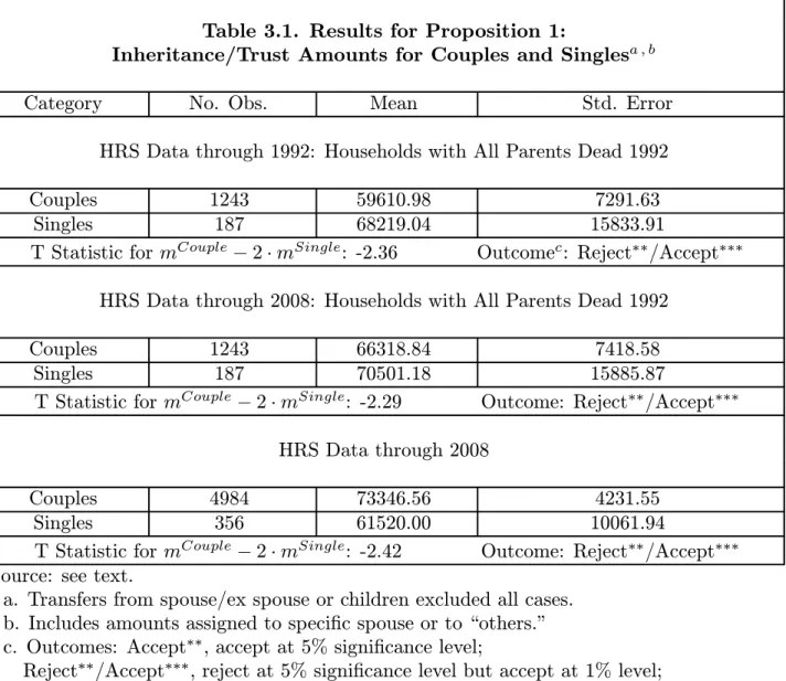
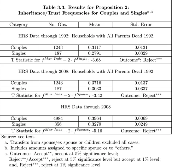
Tables 3.1 and 3.3 present tests of the implications of Propositions 1-2. In both tables, we include transfers received from parents, parents-in-law, and “others.” In thefirst case, we compare unconditional mean inheritance/trust amounts for couples and never-married singles. We test mCouple = 2·mSingle, where mCouple is the average receipt amount per couple and mSingle is the same for never-married singles. In the second, we use frequency data, testingfM ar Inds = 2·fSingle, wherefM ar Indsis the combined frequency of transfer receipt for all married individuals, and fSingle is the receipt frequency for never-married singles. If hypothesis (H1) is correct, neither test should reject.
In fact, all of the T-tests in Table 3.1 reject at the 5 percent significance level – although none at the 1 percent level. The tests in the table use symmetric confi -dence intervals. In evaluating (H1), however, our attention focuses on negative values of
mCouple−2·mSingle. The critical value for a 1 percent one-tailed test is 2.33.6 In that case, the first and third panels of Table 2.1 would reject at the 1 percent level.
All of the tests in Table 3.3 reject at the 1 percent significance level, even with sym-metric confidence intervals.
We conclude that we should reject (H1). In other words, we seem to have more than a mislabeling problem with the spousal transfer data.
Tables 3.2 and 3.4 turn to Corollaries 1-2. We expect sharper results when we consider individual spouses instead of couples. That is what we find. In every panel of Table 3.2, we accept the equality of inheritance amounts for financial respondents in couples and never-married singles. But, we reject equality for spouses and singles, and for thefinancial respondent in a couple and his/her spouse, at the 1 percent significance level.7 This provides more evidence against hypothesis (H1). And, it supports (H2).
Table 3.4 repeats the tests for frequency data. The rejections seem unambiguous.
6 Given fairly large samples, we obtain critical values from the normal distribution. 7 We develop the means and standard errors in the tables from OLS regressions. The
estimated means for couples, or individuals within couples, and singles are independent. In the case offinancial respondents and their spouses, we run a seemingly unrelated regression (SUR) to find the covariance for the means – needed, for instance, for the T test of
mF in Resp−mSpouse. (The estimated means in the SUR regression are the same as those from OLS.)
Tables 3.1 and 3.3 have the advantage of being able to use transfer receipts from parents and “others.” We must exclude the last from Tables 3.2 and 3.4.8 Transfers from “others” account for 10-20 percent of mean amounts. The comprehensive transfers in the top panel of Table 3.1, for example, are $59,611 and $68,219 for couples and singles, respectively. If we exclude transfers from “others,” thefigures drop to $52,971 and $58,776. We should note as well that our theoretical discussion, strictly speaking, applies only to transfers from parents (which would favor the analysis of Tables 3.2 and 3.4). In any case, Tables 3.1-3.4 are consistent in their test results despite different treatments of inheritances from “others.”
Tables 3.3-3.4 have the advantage of sidestepping problems with censored observations. Table 2.1 notes that a nontrivial number of transfer amounts are missing in the data. Our frequency analysis records all transfers, including those with missing amounts; hence, errors from censoring do not arise. This seems a good reason to prefer Tables 3.3-3.4.
Finally, note that we use weighted data. This seems to have a particularly large effect on figures for never-married singles, where the sample sizes are small. For example, in the top panel of Table 3.1, the unweighted means are $54,609 and $47,140, and the T test changes to Accept∗∗ with the unweighted data. Amounts in the top panel of Table 3.2 change to $36,208, $13,030, and $39,985. While the first test outcome remains the same, the second changes toReject∗∗/Accept∗∗∗. However, the third outcome, with a T-statistic of 3.22, remains Reject∗∗∗. The top panels in Tables 3.3-3.4 change to 0.2808 and 0.2246, and 0.2160, 0.0720, and 0.1818, respectively, with all test outcomes unchanged. This paper prefers the weighted data.
In sum, the evidence against (H1) seems decisive. On the other hand, (H2) seems plausible in terms of average amounts and frequencies, and tests do not reject it.
Thus, the spousal transfer data seems to have an excess of zeros. As a consequence, in determining the mean transfer per couples, it seems desirable to average the mean transfer of singles and financial respondents within couples, or to simply double the amounts for
financial respondents within couples – disregarding data on financial-respondent spouses in all cases. This will tend to make couples’ transfer receipts 33-100 percent larger, on average. For micro analysis, one approach would be to develop a theory of transfer re-ceipt per spouse within couples – and to rely exclusively on data pertaining to financial respondents.
Section 4: Assortative Mating
The distribution of non-financial respondent inheritances in the data seems to have too many zeros. However, we now consider the possibility that positive amounts are accurate in spite of this and that they represent a random sample (conditional on a positive amount). Specifically, we consider the following hypothesis:
8 All survey waves distinguish transfers from parents, parents-in-law, spouse/ex spouse,
and children. The 1992 survey wave also distinguishes transfers from respondent siblings and spouse’s siblings – but later waves often do not. None of the survey waves distin-guish transfers from respondent grandparent transfers versus spouse’s grandparents. Later waves, in fact, do not even list grandparent transfers separately.
(H3. Conditional Accuracy.) Although financial respondents may tend to overlook some transfers from their parents-in-law, the spousal transfers they do report have accurate amounts and constitute a random sample from the spousal distribution.
Conditional Amounts. Consider the conditional distribution of non-financial-respondent transfer receipts.
Under (H3), the mean for non-financial-respondents, conditional on a positive amount, call it m∗Spouses, should equal the conditional mean for financial respondents, say,
m∗F in Resp, and should equal the same for singles,m∗Singles. For all 3 groups, the proba-bility distribution conditional on a positive inheritance is
p∗(i)≡p(i|i= 0) = p(i)
1−p(0) all i= 1,2, ..., I . (3) So, the conditional mean is
m∗ =3
i=0
p∗(i)·x(i). (4)
We have
Proposition 3: Whatever the nature of mating patterns, given (H3), financial
respon-dents, non-financial respondents, and never married singles each have the same conditional mean inheritance, namely, m∗.
Proof: In each case, the conditional probability of a positive inheritance i is p∗(i). So, the conditional mean is m∗.
Evidence. Table 4.1 presents evidence.9 Table 4.1 shows that we can reject (H3) at the 5
percent level in only one case, and never at the 1 percent level. The one rejection involves a comparison of spouses with a small sample of singles. When we compare financial respondents within couples with their spouses, the mean amounts are similar (though the spousal average is always smaller).
In the end, Table 4.1 does not contradict (H3).
Assortative Mating. If we are willing to treat positive spousal transfers as a random sample within the conditional distributionp(j|j = 0), other interesting analysis is possible. We first derive several propositions about what we expect the data to show, and what interpretation one should put on various possible findings. Then we generate statistics from the data.
Restrict attention to households reporting a positive spousal inheritance. If (H3) is valid, the conditional distribution of spousal inheritances – i.e., the distribution for strictly positive inheritances – has density (3), p∗(j), j ≥1, and meanm∗, as in (4). Then
9 For Table 4.1, we run a bivariate regression for couples. The dependent variable is
the sum of inheritances from parents and parents-in-law; one independent variable is a dummy that is 1 for an inheritance from the financial respondent’s parents, the other is 1 for inheritances from the in-laws. We allow separate error variances for parent and in-law transfers. And, for double inheritances, the errors can be correlated. (The correlation coefficients are 0.09, 0.08, and -0.02, respectively.) For couples, we report FGLS estimates.
Proposition 4: Maintain hypothesis (H3). If the distribution of inheritances reflects assortative mating, thenmc|SP >0, the mean inheritance for couples for which thefinancial respondent’s spouse has a positive inheritance, is
mc|SP >0 = 2·m∗.
Alternatively, if the distribution of inheritances reflects random mating, then
mc|SP >0 =m+m∗.
Proof: Suppose assortative mating. The probability that the spouse has indexj isp∗(j). If the spouse has indexj, the household has inheritance 2·x(j). LetN2|SP >0be the number of cases with the spouse having a positive inheritance. In the sample in which allfinancial respondent spouses have positive inheritance, assortative mating implies N2|SP >0 will be the number of couples who inherit. Then
mc|SP >0 = N 2|SP >0· j=0 p∗(j)·2·x(j) N2|SP >0 = 2· 3 j=0 p∗(j)·x(j) = 2·m∗.
Next, suppose random mating. That implies p(i|j) = p(i). So, the probability of household outcome (x(i), x(j)) with j = 0 is p(i|j)·p∗(j) =p(i)·p∗(j). Hence,
mc|SP >0 = N 2|SP >0· j=0 i p(i)·p∗(j)·[x(i) +x(j)] N2|SP >0 = 3 j=0 p∗(j)·[3 i p(i)·x(i) +3 i p(i)·x(j)] = 3 j=0 p∗(j)·[m+x(j)] =m+m∗.
The intuition of Proposition 4 is as follows. The fraction of couples with a positive inheritance for the spouse depends upon unknown reporting errors. To escape the influence of the errors, we limit our attention to households reporting positive spousal sums. The mean spousal inheritance on the restricted set is m∗. With assortative mating and (H3), the total inheritance of each household is exactly twice the inheritance of the spouse. If mating is random, then on the restricted set with a positive spousal inheritance,fi nancial-respondent inheritances recapitulate their entire original distribution. The mean spousal inheritance is m∗, but the meanfinancial respondent inheritance is m.
Still limiting ourselves to the set of couples with positive non-financial-respondent inheritances, we have an analog to Proposition 2:
Proposition 5: Maintain (H3). Let fF R|SP >0 be the fraction financial respondents with
a positive inheritance, on the set with positive spousal inheritances. If mating is assortative, then
fF R|SP >0 = 1.
If mating is random, then
fF R|SP >0 =f .
Proof: Maintain either (H3). LetN2|SP >0 be as in the proof of Proposition 4. Suppose mating is assortative. Then a spousal indexj = 0 implies afinancial respondent inheritance
x(i) =x(j)>0. So, fF R|SP >0 = N 2|SP >0· j=0 p∗(j) N2|SP >0 = 3 j=0 p∗(j) = 1.
Alternatively, assume random mating. Then as in the proof of Proposition 4, house-hold outcome (i , j), j = 0, occurs with probability p(i)·p∗(j). Hence,
fF R|SP >0 = N 2|SP >0 ·i=0 j=0 p(i)·p∗(j) N2|SP >0 = 3 i=0 3 j=0 p(i)·p∗(j) =3 i=0 p(i)·3 j=0 p∗(j) =3 i=0 p(i) =f .
The intuition is as follows. With assortative mating, if the spousal inheritance is posi-tive, thefinancial respondent’s is too. With random mating, a positive spousal inheritance has no implication for thefinancial respondent’s likelihood of a positive inheritance; hence, the probability of a positive inheritance for the financial respondent is f.
Our analysis so far has connected the distribution of inheritances to the mating pattern by tacitly assuming intentional bequests. If some, or all, bequests are accidental – as our review of the literature suggests may well be the case in practice – we need to be more careful.
Consider Section 3’s original examples. In the second scenario, parents of types A, B, and C mate assortatively, yielding parent couples
AA , BB , CC .
If the types are equally prevalent, each couple type has frequency 1/3. Suppose type A
individuals desire bequestx >0 and other types desire 0. With intentional bequests only, couples AA leave 2·x, and other couples leave 0.
Alternatively, suppose that each individual desires to leave nothing, but each acciden-tally falls into state a, with probability 1/3, in very old age and leaves x; falls into state
b with the same probability and leaves 0; or, falls into c with probability 1/3 and leaves nothing. Then possible estate outcomes for couples of type AA cover the set
{aa , ab , ac , ba , bb , bc , ca , cb , cc}.
The actual bequest outcomes are (2·x , x ,0) with probabilities 1/9, 4/9, and 4/9, respec-tively. The same outcomes and probabilities apply to couples BB andCC. So, the overall distribution of outcomes in terms of bequests is identical what happens under intentional bequests and random mating.
This is a general result: assortative mating and intentional bequeathing yields what Propositions 4-5 characterize as the outcome from “assortative mating”; any type of mating and accidental bequeathing yields what the propositions characterize as the outcome from “random mating.”
The existing literature does provide some evidence for assortative mating (Lait-ner [2001]), especially in the case of education. If we maintain the hypothesis that mating is assortative, evidence of a random distribution of inheritances would point to accidental bequests as being the most important.
Evidence. Our empirical analysis focuses on Proposition 5 (because the calculations are more straightforward and because Section 2 suggests that frequency data alleviates cen-soring problems).
The means in Table 4.2 show that the conditional frequency for married financial respondents seems distinctly higher than the conditional frequency of never-married singles. In fact, in the first two panels, the former are twice as large. The tests confirm that differences are significant: we reject “random mating” at the 1 percent level in all cases.
On the other hand, the conditional financial-respondent frequencies are a long way from 1.0. Hence, we also reject “assortative mating” in every case.
Summary. Our theoretical analysis implies that assortative mating and intentional be-quest behavior leads to an assortative-mating pattern of inheritances, whereas either ran-dom mating or accidental bequest behavior leads to a ranran-dom-mating pattern. The existing literature provides some independent support for assortative matching.
In terms of empirical results, our tentative conclusion is that the T tests, and the pattern of the T statistics, support the idea that accidental bequest behavior may be widespread. Nevertheless, the pattern of inheritance receipt does not seem entirely random either. It seems possible that mating is, at least to a degree, assortative and that bequest behavior is, in part, intentional.
Section 5: Inter Vivos Gifts
We next briefly turn to inter vivos gifts.
We can apply the propositions and corollaries of Sections 3-4. Their usefulness in Sections 3-4 depended, however, on the assumption that parents bequeath equally to all of their children – an assumption that the existing literature seems to support. The literature does not necessarily argue the same for inter vivos gifts. In fact, some authors suggest that parents are quite willing to make unequal gifts, perhaps using them to compensate less fortunate children (recall Section 1).
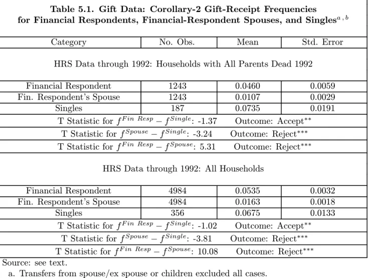
Table 5.1 tests the implications of Corollary 2 on gift data. We limit our sample to cumulative gifts through 1992 (recall Section 2’s discussion). Due to sample size consider-ations, we work with a sample of all couples and singles, as well as one with couples and singles all of whose parents are dead.
Table 5.1 outcomes resemble those of Section 3. The tests accept the idea that singles and financial respondents in couples have the same distribution of gifts, but they reject equality of gift frequencies for singles and financial-respondent spouses, and they reject equality for financial respondents and their spouses. As in Section 3, we believe that
financial respondents in couples are failing to report many of their spouses’ transfers. The degree of misreporting seems, in fact, more severe in the case of gifts (viz., Tables 3.4 and 5.1).
As stated, it seems possible that parents do not divide their gifts equally among their children. However, it seems an unlikely coincidence that inequality of that nature would explain the outcomes of Table 5.1.
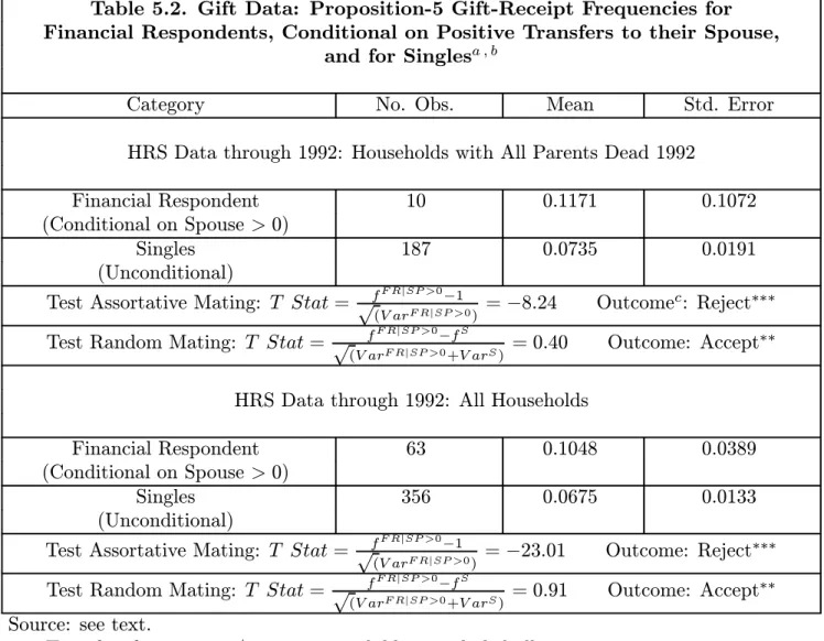
Table 5.2 compares financial-respondent gift receipt, conditional on spousal receipt, with gift-receipt frequencies for singles. As in Section 4, assortative mating is rejected. In contrast to Section 4, however, random mating cannot be rejected.
Nevertheless, a closer look suggests that results from Sections 3-4 carry over. Com-paring Tables 5.1-5.2, financial respondents in couples, conditional on wife’s receipt of a gift, have 2-3 times the chance of receiving a gift as in the unconditional case. Only sample size, it seems, prevents us from rejecting random mating.
In sum, Tables 5.1-5.2 resemble 3.4 and 4.2. This is somewhat surprising. Inheritances may be either intentional or accidental, but inter vivos gifts must, one would imagine, be intentional. If actual mating is assortative and if gifts are intentional, we would expect to accept the lead T test in each panel of Table 5.2. The rejections that we find may then suggest that inter vivos gifts depend on children’s liquidity-constraint problems rather than parental intent to enhance children’s lifetime resources. Or, in conjunction with the evidence on gift timing in Section 2, we might conclude that the gifts reported in our data occur late in parents’ lives and tend to be very similar in character to inheritances – with gifts earlier in life having simply been omitted.
6. Intentional versus Accidental Bequests
In understanding household behavior, the difference between intentional and acciden-tal bequeathing seems important. This section attempts to assess what we can say about the division of actual inheritances between the two categories on the basis of our analysis so far.
Consider Table 4.2, top panel. We now develop an equation for F = 0.4415 = the frequency offinancial-respondent inheritance receipt, conditional of receipt by thefinancial respondent’s spouse. As before, letf be the unconditional frequency of inheritance receipt for an individual. Section 4 argues that we cannot measure f from financial-respondent spouse data. But, we can usefinancial respondent or never-married singles data. Table 4.2
finds f = 0.2293 in the latter case, for instance.
Let z be the fraction of (positive)financial-respondent-spouse inheritances that come from intentional bequests. Then of the fraction f of positive spousal inheritances, z ·f
come from intentional parental transfers, and (1−z)·f from accidental parental transfers. Assume that mating is strongly assortative. Think aboutfinancial respondents whose spouses have positive inheritances. A fraction z of the spouses have intentional parental bequests; so, a fraction z of the conditional financial respondent group does as well. For the remaining fraction of the latter group, 1−z, a share (1−z)·f receive an accidental bequest. Thus, z+ (1−z)2·f =F . (5) We have z+ (1−z)2·f =F ⇐⇒ z+ (1−2·z+z2)·f =F ⇐⇒ f ·z2+ (1−2·f)·z−(F −f) = 0. (6)
A graph shows (6) has a unique non-negative root z whenever F ≥f. If F =f, the root is z = 0. If F = 1, the root is z = 1. The latter two special cases are exactly consistent with Proposition 5.
For F = 0.4415 and f = 0.2293, the unique non-negative root is z = 0.3423. In other words, if all matching is assortative, ourfindings imply that slightly more than 1/3 of HRS inheritances come from intentional parental bequests and 2/3 from accidental bequests.
The frequencies above apply to individuals. For never-married-singles, about 7.5 per-cent inherit from intentional bequests and about 15 perper-cent from accidental bequests – for a total of about 22.5 percent. The same frequencies apply, separately, to married men and married women. Think about a married couple as a unit, however. About 7.5 percent of couples will receive one or more inheritances from intentional bequests. In our simple model, in fact, in each such case both spouses will rceive an intentional transfer. Acciden-tal bequests arrive randomly. Thus, roughly 30 percent of couples will receive 1 or more accidental bequests – with usually only one spouse inheriting in that case. The two types of inheritance are mutually exclusive; so, about 37.5 percent of couples should have at least 1 positive inheritance. We cannot compare the last with any of our tables, since we have argued that spousal inheritances tend to be severely under-reported.
7. Conclusion
In examining HRS data 1992-2008 on private intergenerational transfer receipt, Sec-tion 3finds strong evidence of under-reporting offinancial-respondent spousal inheritances. We recommend disregarding the spousal totals. Careful treatment of this issue can sub-stantially raise one’s assessment of the mean inheritance of couples.
Section 4 presents evidence that the distribution offinancial respondent inheritances, conditional on a positive spousal inheritance, remains valid. The conditional distribution can be very useful. In examining it, we find that we can reject either purely assortative or purely random mating. If we maintain the hypothesis that marital matching is, in fact, assortative, the interpretation of our finding is that actual inheritances represent
a mixture of intentional and accidental bequests, with somewhat greater evidence of the latter. Section 6 carries the analysis further, showing that under the maintained hypothesis of assortative matching, about one-third of individuals’ inheritances seem to originate from intentional bequests, and two-thirds from accidental bequests.
References
[1] Abel, Andrew B., “Precautionary Saving and Accidental Bequests.” American Eco-nomic Review 75 (September 1985): 777-791.
[2] Altonji, J.G., Hayashi, F., Kotlikoff, L.J., “Is the Extended Family Altruistically Linked? Direct Tests Using Micro Data.” American Economic Review 82, no. 5 (1992): 1177-1198.
[3] Altonji, J.G., Hayashi, F., Kotlikoff, L.J., “Parental Altruism and Inter Vivos Trans-fers: Theory and Evidence.” Journal of Political Economy 105, no. 6 (1997): 1121-1166.
[4] Auerbach, Alan J., and Kotlikoff, Laurence J. Dynamic Fiscal Policy. Cambridge: Cambridge University Press, 1987.
[5] Barro, Robert J., “Are Government Bonds Net Wealth?” Journal of Political Econ-omy 82, no. 6 (1974): 1095-1117.
[6] Becker, G.S., “A Theory of Social Interactions.” Journal of Political Economy 82, no. 6 (1974): 1063-1093.
[7] Becker, G.S. Human Capital, Second Edition. Chicago: University of Chicago Press, 1980.
[8] Davies, James B., “Uncertain Lifetime, Consumption, and Dissaving in Retirement.” Journal of Political Economy 89 (June 1981): 561-577.
[9] Dunn, Thomas A., and John W. Phillips, “The Timing and Division of Parental Transfers to Children.” Economics Letters54 (1997): 135-137.
[10] Friedman, B., and Warshawsky, M., “The Cost of Annuities: Implications for Saving Behavior and Bequests.” Quarterly Journal of Economics 105, no. 1 (1990): 135-154. [11] Gale, William G., and John Karl Scholz, “Intergenerational Transfers and the Accu-mulation of Wealth.” The Journal of Economic Perspectives 8, no. 4 (Autumn, 1994): 145-160.
[12] Hurd, Michael, “Savings of the Elderly and Desired Bequests.” American Economic Review 77, no. 3 (1987): 298-312.
[13] Hurd, Michael, “Mortality Risk and Bequests.” Econometrica 57, no. 4 (1989): 779-813.
[14] Kessler, Denis, and Andre Masson, “Bequest and Wealth Accumulation: Are Some Pieces of the Puzzle Missing?” Journal of Economic Perspectives 3 (Summer 1989): 141-152.
[15] Kotlikoff, Laurence J., “Intergenerational Transfers and Savings.” Journal of Eco-nomic Perspectives 2 (Spring 1988): 41-58.
[16] Kotlikoff, Laurence J., and Spivak, Avia, “The Family as an Incomplete Annuities Market.” Journal of Political Economy 89 (April 1981): 372-391.
[17] Kotlikoff, Laurence J., and Lawrence H. Summers, “The Role of Intergenerational Transfers in Aggregate Capital Accumulation.” Journal of Political Economy 89 (Au-gust 1981): 706-732.
[18] Laitner John, “Modeling Marital Connections along Family Lines.” Journal of Polit-ical Economy 99, no. 6 (1991): 1123-1141.
[19] Laitner, John, “Random Earnings Differences, Lifetime Liquidity Constraints, and Altruistic Intergenerational Transfers.” Journal of Economic Theory 58, no. 2 (De-cember 1992): 135-170.
[20] Laitner, John, “Wealth Inequality and Altruistic Bequests.” American Economic Review92, no. 2 (May 2002): 270—273.
[21] Laitner, John, and Juster, F.T., “New Evidence on Altruism: a Study of TIAA-CREF Retirees.” American Economic Review 86, no. 4 (1996): 893-908.
[22] Laitner, John, and Ohlsson, Henry, “Bequest Motives: a Comparison of Sweden and the United States.” Journal of Public Economics79 (2001): 205-236.
[23] Loury, G.C., “Intergenerational Transfers and the Distribution of Earnings.” Econo-metrica 49 (1981): 843-867.
[24] McGarry, Kathleen, “Inter Vivos Transfers and Intended Bequests.” Journal of Public Economics73 (1999): 321-351.
[25] McGarry, Kathleen, and Robert F. Schoeni, “Transfer Behavior in the Health and Re-tirement Study: Measurement and the Redistribution of Resources within the Family.” The Journal of Human Resources 30, Special Issue, 1995: S184-S226.
[26] Menchik, Paul, “Primogeniture, Equal Sharing, and the US Distribution of Wealth.” Quarterly Journal of Economics 94 (March 1980): 299-316.
[27] Menchik, Paul, “Unequal Estate Division: Is It Altruism, Reverse Bequests, or Simply Noise?” In Kessler, Denis, and Andre Masson, eds., Modelling the Accumulation and Distribution of Wealth. Oxford: Clarendon Press, 1988, 105-116.
[28] Modigliani, Franco, “Life Cycle, Individual Thrift, and the Wealth of Nations.” Amer-ican Economic Review76, no. 3 (June 1986): 297-313.
[29] Modigliani, Franco, “The Role of Intergenerational Transfers and Life Cycle Saving in the Accumulation of Wealth.” Journal of Economic Perspectives 2, no. 2 (Spring 1988): 15-40.
[30] Walker, Lina, Three Essays on Retirement Wealth. UM Phd Dissertation, 2005. [31] Wilhelm, Mark O., “Bequest Behavior and the Effect of Heirs’ Earnings: Testing the
Altruistic Model of Bequests.” The American Economic Review86, no. 4 (September 1996): 874-892.
Table 2.1. 1992 HRS Cohort: Cumulative Lifetime Transfers Received through 1992; Unweighted Data
Type of Obs. Mean Standard Minimum Maximum Censored
Transfera Deviation Obs.
Current Dollars; Real Interest Rate = 0
Sample: All HRS households; Cumulative through 1992
Inheritanceb 7702 7750.31 42185.54 1.00 1000000.00 239
Gift 7702 2521.74 20649.67 1.00 1015001.00 80
Life Insurancec 7702 154.72 2141.16 1.00 90000.00 4
Total Transfer 7702 10426.78 51168.09 1.00 1815001.00 313
Sample: Recipient households with positive amount; Cumulative through 1992
Inheritanceb 1400 50458.93 97114.88 1.00 1000000.00 239
Gift 518 43744.29 74790.36 1.00 1015001.00 80
Life Insurancec 69 18333.40 14489.92 1.00 90000.00 4
Total Transfer 1853 50730.92 103411.38 1.00 1815001.00 313
2005 Dollars;d Real Interest Rate = 0
Sample: All HRS households; Cumulative through 1992
Inheritanceb 7702 15729.43 93170.74 1.30 2945508.03 239
Gift 7702 5382.05 50673.17 1.30 3127202.82 80
Life Insurancec 7702 375.33 5603.47 1.39 283768.43 4
Total Transfer 7702 21486.81 118845.36 1.30 5339898.23 313
Sample: Recipient households with positive amount; Cumulative through 1992
Inheritanceb 1400 102407.51 218266.69 1.30 2945508.03 239
Gift 518 93361.53 190601.21 1.30 3127202.82 80
Life Insurancec 69 44473.35 41944.42 1.39 283768.43 4
Total Transfer 1853 104542.88 245025.91 1.30 5339898.23 313
2005 Dollars;d Real Interest Rate = 0.03
Sample: All HRS households; Cumulative through 1992
Inheritanceb 7702 33823.78 221239.02 1.91 6941282.63 239
Gift 7702 11836.15 120813.04 1.91 7572188.63 80
Life Insurancec 7702 926.07 17450.27 2.16 1172602.63 4
Total Transfer 7702 46586.00 282306.66 1.91 12634675.71 313
Sample: Recipient households with positive amount; Cumulative through 1992
Inheritanceb 1400 219469.88 526168.37 1.91 6941282.63 239
Gift 518 205319.93 462022.58 1.91 7572188.63 80
Life Insurancec 69 109732.20 155379.50 2.16 1172602.63 4
Total Transfer 1853 226232.90 588545.77 1.91 12634675.71 313
Source: see text.
a. Transfers from spouse/ex spouse or children excluded all cases. b. Includes trusts.
c. Beneficiary life insurance settlements.
Table 2.2. 1992 HRS Cohort: Cumulative Lifetime Transfers through 1992; 1992 Households Weights
Type of Obs. Mean Standard Minimum Maximum Censored
Transfera Deviation Obs.
Current Dollars; Real Interest Rate = 0
Sample: All HRS households; Cumulative through 1992
Inheritanceb 7585 9132.31 46193.01 1.00 1000000.00 253.21
Gift 7585 3028.02 23572.16 1.00 1015001.00 82.07
Life Insurancec 7585 170.44 2280.97 1.00 90000.00 4.06
Total Transfer 7585 12330.76 65122.82 1.00 1815001.00 327.56
Sample: Recipient households with positive amount; Cumulative through 1992
Inheritanceb 1538.66 52858.88 100196.38 1.00 1000000.00 253.21
Gift 566.42 46642.32 80775.52 1.00 1015001.00 82.07
Life Insurancec 73.10 18725.22 14971.79 1.00 90000.00 4.06
Total Transfer 2019.49 53663.72 127431.37 1.00 1815001.00 327.56
2005 Dollars;d Real Interest Rate = 0
Sample: All HRS households; Cumulative through 1992
Inheritanceb 7585 18418.50 101709.11 1.30 2945508.03 253.21
Gift 7585 6305.04 56615.18 1.30 3127202.82 82.07
Life Insurancec 7585 424.71 5708.20 1.39 283768.43 4.06
Total Transfer 7585 25148.25 149326.55 1.30 5339898.23 327.56
Sample: Recipient households with positive amount; Cumulative through 1992
Inheritanceb 1538.66 106608.49 224665.98 1.30 2945508.03 253.21
Gift 566.42 97120.30 201377.26 1.30 3127202.82 82.07
Life Insurancec 73.10 46659.47 37715.07 1.39 283768.43 4.06
Total Transfer 2019.49 109445.67 296339.60 1.30 5339898.23 327.56
2005 Dollars;d Real Interest Rate = 0.03
Sample: All HRS households; Cumulative through 1992
Inheritanceb 7585 39455.62 240210.50 1.91 6941282.63 253.21
Gift 7585 13635.74 133094.00 1.91 7572188.63 82.07
Life Insurancec 7585 1043.38 16492.51 2.16 1172602.63 4.06
Total Transfer 7585 54134.75 350271.81 1.91 12634675.71 327.56
Sample: Recipient households with positive amount; Cumulative through 1992
Inheritanceb 1538.66 227885.70 538819.42 1.91 6941282.63 253.21
Gift 566.42 210039.45 481255.58 1.91 7572188.63 82.07
Life Insurancec 73.10 114629.11 129856.81 2.16 1172602.63 4.06
Total Transfer 2019.49 235261.43 700415.25 1.91 12634675.71 327.56
Source: see text.
a. Transfers from spouse/ex spouse or children excluded all cases. b. Includes trusts.
c. Beneficiary life insurance settlements.
Table 2.3. 1992 HRS Cohort Inheritances and Trusts: Cumulative Lifetime Transfers Received through 1992; 2005 Dollars,
Real Interest Rate = 0.03, Recipient Households with Positive Amounts; Unweighted Data
Type of Obs. Mean Standard Minimum Maximum Censored
Transfera Deviation Obs.
Inheritance 1333 192225.08 438342.71 1.91 6941282.63 216 less Trusts Transferred 98 572035.65 1007165.79 1.91 5195563.72 29 Trust Accounts Total 1400 219469.88 526168.37 1.91 6941282.63 239 Inheritance/Trust Source: see text.
Table 2.4. The Timing of Inheritances vs Gifts for 1992 HRS Cohort: Cumulative Lifetime Transfers Received through 1992; Unweighted Data
Type of Transfera 1950s 1960s 1970s 1980-92 Total
Frequency of Receipt
Inheritance/Trust 41 135 397 1132 1705
Gifts 14 53 123 467 657
Fraction of Cumulative Total
Inheritance/Trust 0.024 0.079 0.233 0.664 1.000
Gifts 0.021 0.081 0.187 0.711 1.000
Table 2.5. 1992 HRS Cohort: Cumulative Lifetime Transfers Received through 2008; 1992 Household Weights
Type of Obs. Mean Standard Minimum Maximum Censored
Transfera Deviation Obs.
Current Dollars; Real Interest Rate = 0
Sample: All HRS households; Cumulative through 2008
Inheritanceb 7585 28947.89 121960.18 1.00 5114500.00 528.63
Gift 7585 3255.72 24388.48 1.00 1015001.00 87.66
Life Insurancec 7585 170.44 2280.97 1.00 90000.00 4.06
Total Transfer 7585 32374.05 147944.12 1.00 5114500.00 604.71
Sample: Recipient households with positive amount; Cumulative through 2008
Inheritanceb 2701.92 91294.30 203021.81 1.00 5114500.00 528.63
Gift 609.23 46366.52 80448.42 1.00 1015001.00 87.66
Life Insurancec 73.10 18725.22 14971.79 1.00 90000.00 4.06
Total Transfer 3047.82 90314.44 236277.33 1.00 5114500.00 604.71
2005 Dollars;d Real Interest Rate = 0
Sample: All HRS households; Cumulative through 2008
Inheritanceb 7585 40051.75 160320.38 0.92 5133858.85 528.63
Gift 7585 6550.82 57157.77 1.06 3127202.82 87.66
Life Insurancec 7585 424.71 5708.20 1.39 283768.43 4.06
Total Transfer 7585 47027.27 210787.13 0.92 5344017.78 604.71
Sample: Recipient households with positive amount; Cumulative through 2008
Inheritanceb 2701.92 126313.07 264884.19 0.92 5133858.85 528.63
Gift 609.23 93293.83 196047.77 1.06 3127202.82 87.66
Life Insurancec 73.10 46659.47 37715.07 1.39 283768.43 4.06
Total Transfer 3047.82 131192.79 336018.78 0.92 5344017.78 604.71
2005 Dollars;d Real Interest Rate = 0.03
Sample: All HRS households; Cumulative through 2008
Inheritanceb 7585 64254.17 282246.43 0.84 6941282.63 528.63
Gift 7585 13913.35 133516.46 1.12 7572188.63 87.66
Life Insurancec 7585 1043.38 16492.51 2.16 1172602.63 4.06
Total Transfer 7585 79210.90 395172.56 0.84 12638918.84 604.71
Sample: Recipient households with positive amount; Cumulative through 2008
Inheritanceb 2701.92 202382.60 472187.94 0.84 6941282.63 528.63
Gift 609.23 198147.71 466233.37 1.12 7572188.63 87.66
Life Insurancec 73.10 114629.11 129856.81 2.16 1172602.63 4.06
Total Transfer 3047.82 220726.35 635545.15 0.84 12638918.84 604.71
Source: see text.
a. Transfers from spouse/ex spouse or children excluded all cases. b. Includes trusts.
c. Beneficiary life insurance settlements.
Table 2.6. 1992 HRS Cohort: Parent vs In-Law-Parent Benefactors; Unweighted Data
Type of Transfers From Othersc Parents Transfers
Transfera From In-Law ÷In-Law per Household
Parents Parents Parents with Positive
Amount All 1992-Cohort HRS Households: Sample=7702
Cumulative through 1992
Inheritance/Trust 972 200 434 4.86 1.15
Total Transferb 1264 282 589 4.48 1.15
Cumulative through 2008
Inheritance/Trust 1616 596 856 2.71 1.26
1992-Cohort HRS Married Couples: Sample=5009 Cumulative through 1992
Inheritance/Trust 682 192 315 3.55 1.17
Total Transferb 896 269 424 3.33 1.17
Cumulative through 2008
Inheritance/Trust 1141 563 637 2.03 1.29
1992-Cohort HRS Never Married Singles: Sample=356 Cumulative through 1992
Inheritance/Trust 43 0 22 NA 1.12
Total Transferb 61 0 33 NA 1.12
Cumulative through 2008
Inheritance/Trust 75 0 41 NA 1.21
1992-Cohort HRS Married Couples with All Parents Dead 1992: Sample=1250 Cumulative through 1992
Inheritance/Trust 270 90 76 3.00 1.24
Total Transferb 316 105 109 3.01 1.23
Cumulative through 2008
Inheritance/Trust 288 107 155 2.69 1.29
1992-Cohort HRS Never Married Singles with All Parents Dead 1992: Sample=187 Cumulative through 1992
Inheritance/Trust 34 0 14 NA 1.14
Total Transferb 43 0 22 NA 1.12
Cumulative through 2008
Inheritance/Trust 35 0 21 NA 1.22
Source: see text.
a. Transfers from spouse/ex spouse or children excluded all cases. b. Includes inheritances/trusts, gifts, and life insurance. Not useful after
1992 – see text.
Table 3.1. Results for Proposition 1:
Inheritance/Trust Amounts for Couples and Singlesa , b
Category No. Obs. Mean Std. Error HRS Data through 1992: Households with All Parents Dead 1992 Couples 1243 59610.98 7291.63
Singles 187 68219.04 15833.91
T Statistic for mCouple−2·mSingle: -2.36 Outcomec: Reject∗∗/Accept∗∗∗
HRS Data through 2008: Households with All Parents Dead 1992 Couples 1243 66318.84 7418.58
Singles 187 70501.18 15885.87
T Statistic for mCouple−2·mSingle: -2.29 Outcome: Reject∗∗/Accept∗∗∗ HRS Data through 2008
Couples 4984 73346.56 4231.55 Singles 356 61520.00 10061.94
T Statistic for mCouple−2·mSingle: -2.42 Outcome: Reject∗∗/Accept∗∗∗ Source: see text.
a. Transfers from spouse/ex spouse or children excluded all cases. b. Includes amounts assigned to specific spouse or to “others.” c. Outcomes: Accept∗∗, accept at 5% significance level;
Reject∗∗/Accept∗∗∗, reject at 5% significance level but accept at 1% level; and, Reject∗∗∗, reject at 1% signficance level.
Table 3.2. Results for Corollary 1: Inheritance/Trust Amounts for
Financial Respondents, Financial-Respondent Spouses, and Singlesa , b
Category No. Obs. Mean Std. Error HRS Data through 1992: Households with All Parents Dead 1992
Financial Respondent 1243 39512.15 4974.41 Fin. Respondent’s Spouse 1243 13458.52 4363.52 Singles 187 58776.38 14661.89 T Statistic for mF in Resp−mSingle: -1.24 Outcomec: Accept∗∗
T Statistic for mSpouse−mSingle: -2.96 Outcome: Reject∗∗∗
T Statistic for mF in Resp−mSpouse: 3.85 Outcome: Reject∗∗∗ HRS Data through 2008: Households with All Parents Dead 1992
Financial Respondent 1243 41014.07 5003.15 Fin. Respondent’s Spouse 1243 13938.22 4365.59 Singles 187 58897.90 14659.63
T Statistic for mF in Resp−mSingle: -1.15 Outcome: Accept∗∗
T Statistic for mSpouse−mSingle: -2.94 Outcome: Reject∗∗∗ T Statistic for mF in Resp−mSpouse: 3.98 Outcome: Reject∗∗∗
HRS Data through 2008
Financial Respondent 4984 42776.07 3246.78 Fin. Respondent’s Spouse 4984 16712.16 1987.06 Singles 356 51727.78 9420.85
T Statistic for mF in Resp−mSingle: -0.90 Outcome: Accept∗∗
T Statistic for mSpouse−mSingle: -3.64 Outcome: Reject∗∗∗ T Statistic for mF in Resp−mSpouse: 6.78 Outcome: Reject∗∗∗ Source: see text.
a. Transfers from spouse/ex spouse or children excluded all cases.
b. Includes amounts assigned to specific spouse; excludes amounts assigned to “others.”
c. Outcomes: Accept∗∗, accept at 5% significance level;
Reject∗∗/Accept∗∗∗, reject at 5% significance level but accept at 1% level;