Volume 30, Issue 2
Equity premium under multiple background risks
Yoichiro Fujii
Graduate School of Systems and Information Engineering, University of Tsukuba
Yutaka Nakamura
Graduate School of Systems and Information Engineering, University of Tsukuba
Abstract
In a static Lucas's tree economy, we explore the effect of two types of background risk, uninsurable risk for labor income and miscalibrated risk for payoff distribution of risky asset, on the equilibrium price of the risky asset. Then we analyze the data of U.S. stock market and GDP growth rates during 1871-2004 to verify that our simple static model could provide appropriate magnitudes of equity premium.
Citation: Yoichiro Fujii and Yutaka Nakamura, (2010) ''Equity premium under multiple background risks'', Economics Bulletin, Vol. 30 no.2 pp. 933-939.
1. Introduction
It was pointed out by Mehra and Prescott (1985) that the representative agent model in a Lucas (1978) tree economy dramatically underestimates the equity premium. In a two-period version of Lucas economy, Weil (1992) examined whether or not the existence of uninsurable background risk, such as a risk on labor income, could explain the equity premium puzzle. He showed that if preferences exhibit standardness (i.e., decreasing absolute risk aversion and decreasing absolute prudence), then the magnitude of the equity premium is increased. The question is whether or not it yields a sizable e®ect.
Recently, in a static Lucas economy, Gollier (2001) examined a simpli¯ed version of Weil model by adding a background risk to initial wealth, and concluded that the existence of idiosyncratic background risk, when considered in isolation, cannot explain the equity risk premium puzzle, that is, the model cannot yield a sizable e®ect. On the other hand, Gollier and Schlesinger (2002) attached the background risk to the initial asset-payo® distribution, rather than to initial wealth. They showed how such a miscalibration of risk, together with an assumption that preferences are standard, o®ers a new potential explanation for empirically high equity premium.
This article further elaborates Gollier-Schesinger's static Lucas model by adding back-ground risks to both of initial wealth and asset-payo® distribution. Thus we explore the e®ect of two types of background risk, uninsurable risk for labor income and miscalibrated risk for payo® distribution of risky asset, on the equilibrium price of the risky asset. We analyze the data of U.S. stock market and GDP growth rates during 1871-2004 and estimate the magnitude of the equity premium. Our calibrations show that the impact of unisurable risk on the magnitude of the equity premium is much smaller than miscalibrated risk, and verify that our simple static model could provide appropriate magnitudes of equity premium with the observed standard deviation 9% of labor income risk when the standard deviation of miscalibrated risk is between 3% and 8%, depending on the relative risk aversion coe±cients.
2. Equilibrium Prices under Multiple Background Risks
Consider a static Lucas tree economy consisting of risk-averse individuals, all of whom may be portrayed by a representative agent. Let u denote the representative agent's von Neumann-Morgenstern utility function over the ¯nal wealths. In addition to the one unit of physical capital, each agent in the economy is endowed with some initial human capital. Let ~
xdenote the revenue generated by each unit of physical capital, which is perfectly correlated across ¯rms. The revenue generated by the human capital is denoted by ~w. We assume that it is independently distributed across agents, and that it is also independent of ~x. Following
Gollier and Schlesinger (2002), the equilibrium price of ~x will be equal to
Pu;w~(~x) =
Exu~ 0( ~w+ ~x) Eu0( ~w+ ~x) ;
the equity premium in this economy will be equal to
Áu;w~(~x) = Ex~
Pu;w~(~x) ¡
1:
Now we shall consider two types of background risks, ~²x and ~²w, and replace ~x and ~w by
~
x+ ~²x and w0+ ~²w, respectively, in the equilibrium price formula, where E~²x =E~²w = 0 and
~
x, ~²x, and ~²w are independent. Assuming thatu exhibits standardness, it easily follows from
the results of Weil (1992) and Gollier and Schlesinger (2002) that two distinct background risks together reduce the equilibrium price more than any one of those risks, i.e., for all ~x,
Pu;w0+~²w(~x+ ~²x)< ( Pu;w0+~²w(~x) Pu;w0(~x+ ~²x) ) < Pu;w0(~x): (1)
Weil (1992) proved the upper second inequality in (1), and interpreted background risk ~²w
as private information and therefore uninsurable due to observability asymmetries. Gollier and Schlesinger (2002) attached the \noise" term ~²x to the original asset distribution ~x to
extend Weil's argument for the equity-premium puzzle under miscalibrated risk, and proved thatPu;w0(~x+ ~²x)< Pu;w0+~²w(~x) when ~²x = ~²w in the middle of (1). Assume that the market
analyst calculates a sampling distribution function of the true distribution for ~x, which is based on historical data. If consumers all possess the same distributional information as the analyst, but consumers include a spurious noise term ~²x in their estimated distribution,
they argued that the lower second inequality in (1) follows from Weil's result, that is, the analyst's estimated equilibrium pricePu;w0(~x) is higher than the empirical equilibrium price
Pu;w0(~x+ ~²x). This, of course, leads to a higher empirical equity premium than the analyst's
prediction. Hence, they have another potential explanation for the equity premium puzzle. However, in general, it is not clear which of Pu;w0+~²w(~x) (Weil's e®ect) andPu;w0(~x+ ~²x)
(GS e®ect) is larger than the other unless ~²w = ~²x. By the ¯rst inequality in (1), we may
interpret that a market analyst who ignores the uninsurable risk ~²w and calculates price
according to a sampling distribution of the true distribution for ~x will overestimate the empirical equilibrium price Pu;w0+~²w(~x+ ~²x) in a market with two distinct background risks
~
²w and ~²x which is also strictly smaller than the equilibrium prices due to Weil's e®ect and
3. Numerical Analyses
For simplicity, we assume that w0 = 0. Then we interpret ~x as the random variable
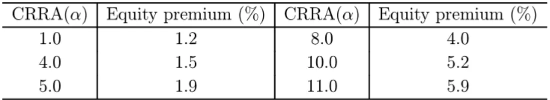
representing the GDP per capita. Taking the time series of the growth rate of U.S. real GDP per capita for the period from 1871 to 2004 (average, 2:1%; standard deviation, 5:4%; maximum value, 18:7% in 1942; minimum value, ¡21:5% in 1946; see Maddison, 2007), we assume that agents believe that each realized growth rate in the past will occur with equal probability, and that agents have a constant relative risk aversion (CRRA)®. Then using the formula Áu;0(~x), we can calculate the equity premium in the static Lucas economy. Several
empirical studies about U.S. stock markets (e.g., Merton, 1980; Pindyck, 1988; Finn, et al., 1990; Klock and Phillips, 1999; TÄodter, 2008) show that the range of estimated value of ®
may be given by an interval [1;8]. Table 1 reports various equity premiums Áu;0(~x) as a
function of ®.
Table 1. Equity premiums with CRRA and ~xbased on the actual growth rates of U.S. real GDP per capita, 1871-2004
CRRA(®) Equity premium (%) CRRA(®) Equity premium (%)
1:0 1:2 8:0 4:0
4:0 1:5 10:0 5:2
5:0 1:9 11:0 5:9
Over the period 1871-2004, we take the real returns of S&P500 and interest rates, which are respectively regarded as risky and risk-free assets in our model. The averages of the real return of S&P500 and the interest rates are respectively 8:2% and 2:9% per year (see Shiller, 2005). Hence we obtain that the average of equity premiums over the period is around 5:3%. Clearly, this simple static version of Lucas tree economy does not ¯t the data1 for 1·®·8.
To bridge the gap, we shall calculate the e®ects of background risks on the sizes of equity premium. For computational simplicity, we assume that labor income risk ~²w is distributed
1Surprisingly, the puzzle disappears under the static model if®
¸10. Mehra and Prescott (1985) used data of consumption per capita over the period 1889-1978. They obtained that, for®·10, the maximum estimated equity premium is 0:35%. On the other hand, Gollier (2001) used GDP growth rates over the period 1963-1992. He obtained that, for ®·10, the maximum estimated equity premium is 0:61%. Thses estimated values are ten times smaller than the values in Table 1. This may be due to two empirical ¯ndings: smaller standard deviation of concumption data than GDP and smaller sandard deviation for shorter period.
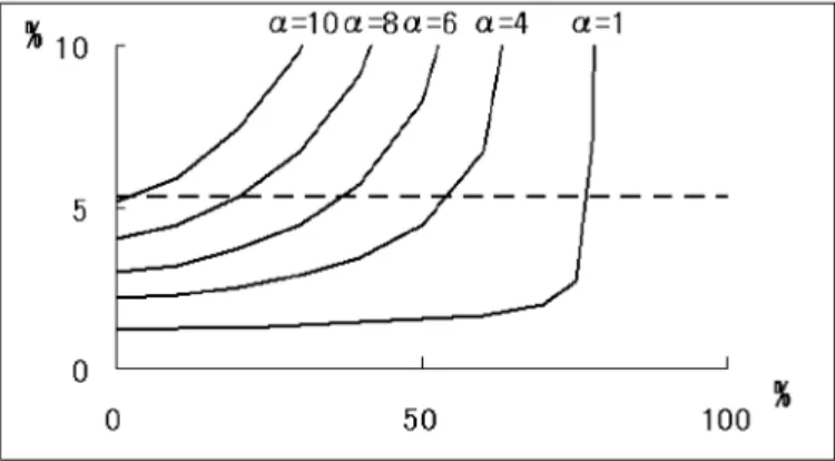
Figure 1: Equity Premium (vertical line) and labor income risk (horizontal line)
Figure 2: Equity Premium (vertical line) and miscalibrated risk (horizontal line)
asD¡k;1 2; +k;
1 2 E
for somek >0, where value +kobtains with probability 1=2 and value¡k
obtains with probability 1=2. Parameter k is the standard deviation of the growth of labor incomes. Using the historical frequency of the growth of GDP per capita for ~x and CRRA utility functions with ® = 1 » 10, we obtain the equity premium Áu;~²w(~x) as a function of
the sizek of the uninsurable risk. Figure 1 shows these numerical results, where the dashed horizontal line depicts the level of equity premium obtained in the preceding paragraph. We see that a very large background risk is required to explain the puzzle, for example, with a standard deviation of the annual growth of individual labor income exceeding 20% for®·8. Now we numerically verify our modi¯cation of Gollier and Schlesinger's static Lucas model in U.S. stock market. Although growth rates of annual earnings in U.S. manufacturing were not available over the period 1871-2004, we assume from NBER and Penn World that the standard deviation of the growth rates is 9%. Thus we let k = 0:09, so that
~
²w = D
¡0:09;12; +0:09;12Erepresents labor income risk. Let us also assume that background risk ~²x is distributed as D ¡n;1 2; +n; 1 2 E
for somen >0. Parameternis the standard deviation of the miscalibrated risk of the asset-payo® distribution ~x. As in the preceding paragraph, we can calculate the equity premiumÁu;~²w(~x+~²x) as a function of the sizenof the miscalibrated
risk.
In Figure 2, these calculations are presented in two cases of k = 0:09 (dashed curves) and k = 0 (real curves). The latter case is exactly the results from Gollier-Schlesinger model. We see that Weil's e®ect is much smaller than GS e®ect. We may conclude that a mild background risk ~²x, whose standard deviation is between 3% and 8% depending on ® = 4 » 8, is su±cient to explain the puzzle. For 1 · ® < 4, however, larger parameter valuesn(10%»20%), which may blur out a sampling distribution function of ~x, are required to reduce the equilibrium price.
4. Conclusion
The aim of this article was to further elaborate Gollier and Schlesinger's simpli¯ed ver-sion of a static Lucas model. Introducing two types of background risk in the model, we demonstrated that our version reduces equilibrium price of risky asset more than each one of Weil's e®ect and GS e®ect. Then we analyzed U.S. stock markets during 1871-2004 to verify that the estimated equilibrium price is small enough to explain the equity premium puzzle for ®= 4 »8. It also follows from our calibration that Weil's e®ect is much smaller than GS e®ect. It may be theoretical interest to investigate this large di®erence of e®ects of background risks on the equilibrium price.
References
Abdulkadri, A.O. and Langemeier, M.R. (2000) Using farm consumption data to esti-mate the intertemporal elasticity of substitution and relative risk aversion coe±cients.
Agricultural Fiance Review 60, 61-70.
Finn, M.G., Ho®,an, D.L., and Schlangenhauf, D.E. (1990) Intertemporal asset pricing relationships in barter and monetary economies: an empirical analysis. Journal of Mon-etary Economics 25, 431-451.
Gollier, C. and H. Schlesinger. (2002) Changes in risk and asset prices, Journal of Mon-etary Economics 49, 747-760.
Klock, M. and Phillips, R.F. (1999) A model of reform volatility with application to estimating relative risk aversion. Review of Quantitative Finance and Accounting 13, 249-260.
Lucas, R.E. (1978) Asset prices in an exchange economy, Econometrica 46, 1429-1446. Maddison, A. (2007) Contours of World Economy 1-2030 AD, Oxford University Press (Data is available at http://www.ggdc.net/maddison/)
Mehra, R. and E. Prescott. (1985) The equity premium: a puzzle, Journal of Monetary Economics 15, 145-161.
Pindyck, R.S. (1988) Risk aversion and determinants of stock market behavior. Review of Economics and Statistics 70, 183-190.
Shiller, R. (2005) Irrational Exuberance. 2nd ed., Princeton University Press (Data is available at http://www.econ.yale.edu/~shiller/)
TÄodter, K.H. (2008) Estimating the uncertainty of relative risk aversion. Applied Finan-cial Economics Letters 4, 25-27.
Merton, R.C. (1980) On estimating the expected return on the market: an exploratory investigation. Journal of Financial Economics 8, 323-361.
Weil, P. (1992) Equilibrium asset prices with undiversi¯able labor income risk, Journal of Economic Dynamics and Control 16, 769-790.