Course Notes: Nonlinear Dynamics and Hodgkin-Huxley Equations

Reading: Hille (3rd

ed.), chapts 2,3; Koch and Segev (2nd

ed.), chapt 7 (by Rinzel and Ermentrout). For further reading, S.H. Strogatz, Nonlinear Dynamics and Chaos, Addison Wesley, 1994.

In these lectures introductory ideas of nonlinear dynamics are used to illustrate the properties of membrane models based on the Hodgkin Huxley (HH) equations. The idea of reducing a system to second order is introduced and applied to generate models that can be analyzed in the phase plane.

Hodgkin-Huxley modeling

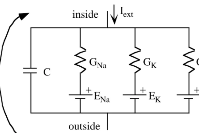
The basic membrane circuit is drawn in Fig. 1. This circuit is appropriate for simple membrane systems like the squid giant axon or other axonal membranes, where only two voltage-dependent channels are seen. In the model there is a capacitor C, to represent the membrane capacitance, a sodium conductance GNa, potassium conductance GK,

and a leakage conductance GL. The

membrane potential V is the potential inside the cell minus the potential outside and there can be a current Iext injected into the cell from

an electrode or from other parts of the cell.

Consistent with the usual convention, currents are positive in the outward direction.

The model in Fig. 1 represents a patch of membrane, i.e. a small area of membrane which is isopotential, meaning that the membrane potential V is constant across the patch. In the last part of the course, we will consider more general models in which the voltage varies along the extent of the cell. Patch models are appropriate for systems consisting of a large number of channels relatively evenly dispersed across the patch. More specifically, two things are assumed: 1) the number of channels is large enough that individual gating events are averaged out and the Na and K currents are smooth population currents (see Figs. 3.16 and 3.17 in Hille); and 2) the channels are not arranged in any way which allows special local interactions among small numbers of channels. Such interactions most frequently occur between calcium channels and other channel types through local calcium pools. In this model, the channels interact only through V.

The equations describing the patch in Fig. 1 were first developed by Hodgkin and Huxley (HH, 1952). Conservation of current at the node on the inside of the cell gives:

CdV

dt =Iext−GNa(V−ENa)−GK1(V−EK)−G VL( −EL) (1) Fig. 1 Typical membrane circuit containing active Na and K channels, a leakage channel and a membrane

+ C GNa GK GL E_Na +E_K +E_L I_ext inside outside V

That is, the current through the capacitance is the externally applied current minus the currents through the ion channels. C and GL are constants. GNa and GK are functions of membrane potential

and time, given the following HH equations:

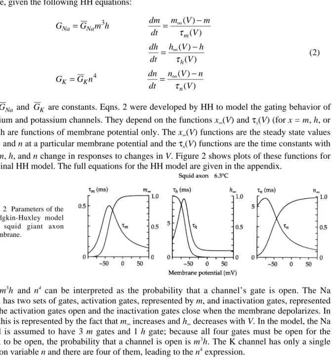
G G m h dm dt m V m V dh dt h V h V G G n dn dt n V n V Na Na m h K K n = = − = − = = − ∞ ∞ ∞ 3 4 ( ) ( ) ( ) ( ) ( ) ( ) τ τ τ (2)

where G_Na and G_K are constants. Eqns. 2 were developed by HH to model the gating behavior of the sodium and potassium channels. They depend on the functions x_∞(V) and τx(V) (for x = m, h, or

n) which are functions of membrane potential only. The x_∞(V) functions are the steady state values of m, h, and n at a particular membrane potential and the τx(V) functions are the time constants with which m, h, and n change in responses to changes in V. Figure 2 shows plots of these functions for the original HH model. The full equations for the HH model are given in the appendix.

m3

h and n4

can be interpreted as the probability that a channel’s gate is open. The Na channel has two sets of gates, activation gates, represented by m, and inactivation gates, represented by h. The activation gates open and the inactivation gates close when the membrane depolarizes. In Fig. 2, this is represented by the fact that m_∞ increases and h_∞ decreases with V. In the model, the Na channel is assumed to have 3 m gates and 1 h gate; because all four gates must be open for the channel to be open, the probability that a channel is open is m3h. The K channel has only a single

activation variable n and there are four of them, leading to the n4

expression.

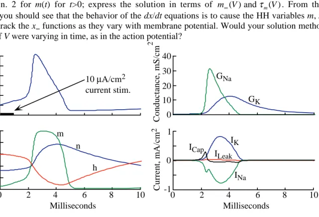
Figure 3 shows the evolution of the parameters of the HH model during an action potential. Explanations of the action potential based on this model are given in the references (Hille, chapter 2 and Johnston and Wu, chapter 6) and will not be repeated here. Instead, these notes focus on developing an understanding of the properties of nonlinear systems like the HH equations using the phase-plane approach from nonlinear dynamics.

Question 1. Assume that the membrane potential has been fixed at V0 for a long time. What

is the steady state value of m? At time 0, the membrane potential is stepped (voltage-clamped) to V1. Fig. 2 Parameters of the

Hodgkin-Huxley model for squid giant axon membrane.

Solve Eqn. 2 for m(t) for t>0; express the solution in terms of m V_∞( ) and τm( )V . From this solution, you should see that the behavior of the dx/dt equations is to cause the HH variables m, n, and h to track the x_∞ functions as they vary with membrane potential. Would your solution method be valid if V were varying in time, as in the action potential?

0 10 20 30 40 G_K G_Na Conductance, mS/cm 2 -80 -40 0 40 Membrane pot., mV 0 0.4 0.8 HH variables 10 µA/cm2 current stim. 0 2 4 6 8 10 Milliseconds 0 2 4 6 8 10 Milliseconds m n h -1 0 1 Current, mA/cm 2 I_K I_Na I_Leak I_Cap

Question 2. There is a notch in the sodium current (INa) in the lower right plot of Fig. 3. It

occurs about the time the sodium conductance ( GNa) reaches its peak. Explain the origin of the

notch. Similarly, the shape of the potassium current waveform (IK) is different from the potassium

conductance waveform (GK). Explain why.

Question 3. HH considered m, h, and n to specify the fraction of gating elements that were

open in the two channel types. Each gating element could undergo transitions from closed to open according to the following first-order kinetic scheme

C αx O

(V) βx(V)

(3)

where C and O are closed and open states and α and β are voltage-dependent rate constants for the opening and closing transitions, respectively. Derive expressions for x_∞(V) and τx(V) in terms of

αx(V) and βx(V). The HH model is specified in terms of the rate constants αx(V) and βx(V) in the appendix.

Question 4. Taking the four-gate model for the Na channel seriously, gives 24 or 16 possible states for the Na channel (e.g. CCC-C, CCC-O, CCO-C, etc. where the first three symbols, to the left of the dash, represent the states of the m gates and the fourth symbol, to the right of the dash,

Fig. 3 Time course of the important variables in the HH model for nerve action potentials during an action potential. Shown are the membrane potential (upper left), the HH variables (lower left), the conductances (upper right), and the membrane currents (lower right).

represents the h gate). Write out all sixteen states and draw arrows between them to represent the elementary transitions like Eqn. 3. Assume that only one of the four gates changes in each transition, i.e. the likelihood of two gates switching simultaneously is ≈0. Many of these states are equivalent (e.g. OCC-C, COC-C, and CCO-C). Collapse your state diagram and show that it is equivalent to (4) below. Also show that this state model is equivalent to the HH model for the Na channel in Eqn. 2. C3 C2 C1 O I3 I2 I1 I0 3αm(V) βm(V) 2αm(V) _αm(V) 2βm(V) 3βm(V) 3αm(V) βm(V) 2αm(V) α_m(V) 2βm(V) 3βm(V) αh(V) βh(V) βh(V) αh(V) βh(V) αh(V) αh (V) βh(V)

HH models have now been derived for a large number of channels (see Yamada et al., 1998 for examples). Generally the form of the equations is similar to those of Eqn. 2. However, as the detailed study of various channel systems has evolved, some of the features of the HH model have been changed, for both the squid axon (e.g. Clay, 1998) and for other systems (Hille, chapters 18 and 19).

1. For an increasing number of channels, the kinetic scheme of Eqn. 4 has been found to be inaccurate. More complex channel state models are needed and these can now be derived from single channel recordings. This means that explicit differential equations for the state model have to be written and these usually cannot be collapsed into the compact form of the HH equations (Eqn. 2). This change in the model generally reflects subtle changes in the gating behavior of channels.

2. The HH model assumes that the instantaneous current-voltage relationship of a channel is linear, i.e. that Ix=Gx(V,t)

.

(V-Ex). As discussed in the notes on channel permeation models, the

current-voltage relationship does not necessarily take this linear form. Usually a more accurate instantaneous current voltage model is the Goldman-Hodgkin-Katz constant field equation:

I m h V C e C e i p q inside z FV RT outside z FV RT i i =

[

]

where m and h are HH variables as in Eqn. 2 and Eqn. 5 is substituted for the linear current voltage relationships in Eqn. 1. Equation 5 is most commonly used in modeling Ca++ channels, because the large concentration ratio Cout/Cin leads to strong rectification. In these notes, the

linear form of the equation, i.e. Eqn. 1, will be used for simplicity of analysis.

State variable models and reduced-state models: the Morris-Lecar Equations

The state variables of the HH model are V, m, h, and n. These form the state vector r

X=[ , , , ] and the differential equations (Eqns. 1 and 2) can be written as follows:V m h nT

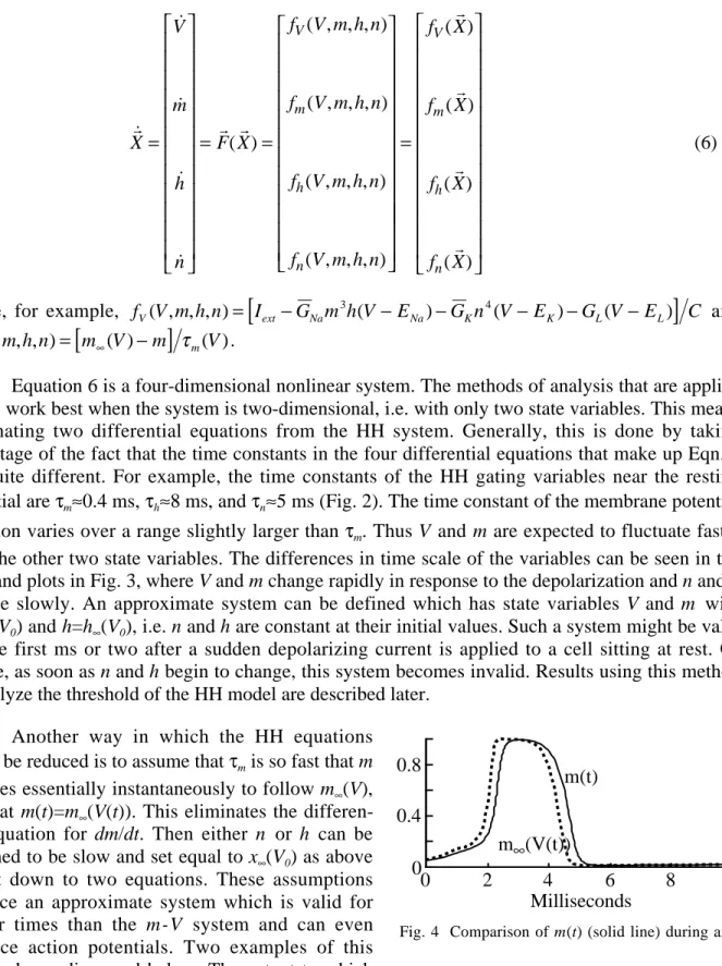
r_˙ r r ˙ ˙ ˙ ˙ ( ) ( , , , ) ( , , , ) ( , , , ) ( , , , ) X V m h n F X f V m h n f V m h n f V m h n f V m h n V m h n =                             = =                             =                             f X f X f X f X V m h n ( ) ( ) ( ) ( ) r r r r (6)

where, for example, f V m h nV( , , , )=

[

]

3 4

and

f V m h nm( , , , )=

[

]

Equation 6 is a four-dimensional nonlinear system. The methods of analysis that are applied below work best when the system is two-dimensional, i.e. with only two state variables. This means eliminating two differential equations from the HH system. Generally, this is done by taking advantage of the fact that the time constants in the four differential equations that make up Eqn. 6 are quite different. For example, the time constants of the HH gating variables near the resting potential are τm≈0.4 ms, τh≈8 ms, and τn≈5 ms (Fig. 2). The time constant of the membrane potential equation varies over a range slightly larger than τm. Thus V and m are expected to fluctuate faster than the other two state variables. The differences in time scale of the variables can be seen in the left hand plots in Fig. 3, where V and m change rapidly in response to the depolarization and n and h change slowly. An approximate system can be defined which has state variables V and m with

n=n_∞(V0) and h=h∞(V0), i.e. n and h are constant at their initial values. Such a system might be valid

for the first ms or two after a sudden depolarizing current is applied to a cell sitting at rest. Of course, as soon as n and h begin to change, this system becomes invalid. Results using this method to analyze the threshold of the HH model are described later.

Another way in which the HH equations might be reduced is to assume that τm is so fast that m changes essentially instantaneously to follow m_∞(V), i.e. that m(t)=m_∞(V(t)). This eliminates the differen-tial equation for dm/dt. Then either n or h can be assumed to be slow and set equal to x_∞(V0) as above

to get down to two equations. These assumptions produce an approximate system which is valid for longer times than the m-V system and can even produce action potentials. Two examples of this approach are discussed below. The extent to which

the assumption about m is true for the HH equations can be judged from Fig. 4 which compares the actual trajectory of m during an action potential (solid line) with the trajectory of m_∞ (dashed line).

Fig. 4 Comparison of m(t) (solid line) during an

∞ 0 2 4 6 8 10 0 0.4 0.8 m(t) Milliseconds m_∞(V(t))

As expected from Eqn. 2, m_∞ leads m. The approximation of holding either h or n constant can be evaluated from the lower left plot in Fig. 3.

For the initial discussion of phase-plane analysis, a two-dimensional set of equations similar to the reduced HH equations will be used. These are the Morris-Lecar equations (MLE) in the form used by Rinzel and Ermentrout (1998). The membrane model of Fig. 1 is still appropriate, except that the model contains a calcium channel instead of the sodium channel. The calcium activation variable, m, is assumed to have a fast time constant, so that m=m_∞(V) and the calcium conductance is G_Ca =G_Cam_∞( ) . There is no calcium inactivation variable, which is equivalent to assumingV

that h is constant. The potassium channel has a single activation variable w, analogous to n, so the state variable equations are as follows:

CdV dt I G m V V E G w V E G V E dw dt w V w V ext Ca Ca K K L L w = − − − − − − = − ∞ ∞ ( )( ) ( ) ( ) ( ) ( ) φ τ (7) where m V V V V w V V V V V V V V w ∞ ∞ =

[

(

(

)

)

]

[

(

(

)

)

]

(

)

(

)

The functional forms chosen for m_∞, w_∞, and τw have the same general shape as the analogous parameters of the HH model and have the advantage that they are easy to compute. The parameter φ in Eqn. 7 is a temperature factor, which can be used to change the relative time constants of V and

w. Experimentally, the time constants of channel gating (dw/dt) are more sensitive to changes in

temperature than the time constant of dV/dt.

The model will be used with two sets of parameters:

Parameter set #1 G_Ca=4.4 G_K=8.0 G_L=2.0 C=20 ECa=120 EK=-84 EL=-60 φ=0.04 (9) V1=-1.2 V2=18 V3=2 V4=30 Parameter set #2 G_Ca=4.0 G_K=8.0 G_L=2.0 C=20 ECa=120 EK=-84 EL=-60 φ=0.0667 (10) V1=-1.2 V2=18 V3=12 V4=17.4

Units are mV for potentials, mS/cm2

for conductance, µA/cm2

for current, and µFd/cm2

for capacitance. Iext will be varied to simulate current input to the cell.

-60 -40 -20 0 20 40 V, membrane potential, mV) w , potassium activation 0.6 0.4 0.2 0 dV/dt=0 dV/dt=0 dw/dt=0 x x x

The phase plane

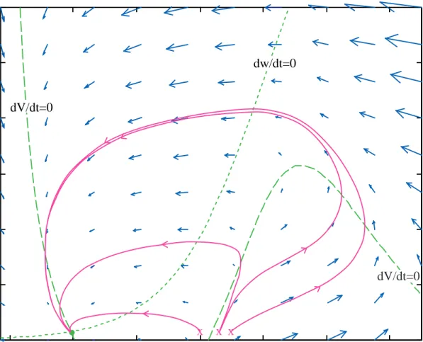
Because Eqns 1 and 2 and Eqns 7 and 8 are nonlinear, it is not possible to obtain solutions except by numerical simulation. However, considerable insight into the nature of the solutions can be gotten using simulation and phase plane analysis. A phase plane, for an order 2 system like Eqn. 7, is a Cartesian plot with the state variables on the axes. Figure 5 shows an example for the MLE with parameter set #1. There are several features in this plot, which will be described one by one.

At each point (V, w) in the plane, the velocity vector (dV/dt, dw/dt) can be computed from Eqn. 7. The blue arrows show these velocity vectors on an evenly spaced grid in the plane. The vectors point in the direction that the solutions to Eqn. 7 will move if the system’s state vector is located at the tail of the arrow; the length is the speed of movement. A great deal about the nature of the system’s behavior can be inferred from the arrows. Indeed, the process of simulation to obtain solutions is basically computing these arrows on a sufficiently dense grid and then following the arrows.

Fig. 5. Phase plane for the MLE with parameter set #1. The green dashed lines are the nullclines dw/dt=0 and dV/dt=0. The blue arrows show the directions and flow velocities of trajectories at the points corresponding to the tails of the arrows. The magenta solid lines are example trajectories for V0=-20 mV, -14 mV, -13.9 mV, and

The solid magenta lines show actual trajectories for the system from four initial points (the x’s). That is, Eqns. 7 and 8 were solved numerically with the initial conditions V(0)=-20, -14, -13.9, and –10 mV and w(0)=0.014915 (its value at the resting point). Plots of the resulting time functions

V(t) and w(t) are shown in Fig. 6 for two of the initial conditions (-14 and -13.9 mV). The magenta

trajectories in Fig. 5 are plots of w(t) versus V(t) with time t as a parameter. Time is not explicitly marked on the trajectories and there is no necessary relationship between distance along the trajectories and the passage of time. Notice in Fig. 2 that the trajectories follow the directions predicted by the blue arrows. All four trajectories end up at the green dot (V=-61.2 mV, w=0.0149), which is the resting state of the model.

0 20 40 60 80 -80 -40 0 100 Time, ms. V , mV 40 0 20 40 60 80 100 Time, ms. V(0) = -14 mV V(0) = -13.9 mV V w V w 0 0.2 0.4 0 0.2 0.4 w , potassium activation -80 -40 0 40

For initial values of V of –20 and –14 mV, the membrane potential decays directly back to the resting value. This is illustrated by the solution in the left plot of Fig. 6, for –14 mV initial condition. In the phase plane, the trajectories move to the left, back to the resting state (green dot). For the larger initial values (-13.9 and –10 mV), the system produces an action potential, seen in the right plot in Fig. 6. In that case, the trajectory in Fig. 5 moves to the right, eventually returning to the rest state after circling the phase plane. Make sure you understand the relationship between the time plots in Fig. 6 and the trajectories in Fig. 5.

Question 5. The trajectories in Figs. 5 and 6 were computed from an initial value in which

the membrane potential was displaced from the rest potential horizontally, so that w did not change from its value at rest. Show that this manipulation is equivalent to beginning the system at its resting potential and injecting an impulse of current. That is, show that the following are equivalent initial conditions for the MLE (where (V0, w0) is the resting point):

V V w w I t q t V V q C w w I t ext ext ( ) ( ) ( ) ( ) ( ) / ( ) ( ) 0 0 0 0 0 0 0 0 0 = = = = + = = , and versus , and δ

It is worthwhile thinking about how the directions of flow in the phase plane, indicated by the blue arrows in Fig. 5, come about. Consider first the arrows near the V-axis, where w≈0. Moving

Fig. 6. Plots of membrane potential V (blue, left ordinates) and potassium activation w (greeen, right ordinates) versus time for two of the trajectories in Fig. 5 (the two beginning at the middle “x” near –14 mV). The initial voltage value is given in the legend. The dashed lines show the values of V (blue) and w (green) at the resting state

from left to right along the V-axis produces a strong increase in dV/dt, indicated by the increasing length of the right-pointing horizontal component of the arrows. This increase results from the increase in m_∞(V) with V in the second term on the r.h.s. of the dV/dt portion of Eqn. 7 (remember that (V-ECa) is negative), i.e. by the inward calcium current which depolarizes the cell. Moving

vertically anywhere in the phase plane, corresponding to increasing w, yields left-pointing arrows, an effect caused by the third term on the r.h.s. of the dV/dt portion of Eqn. 7, corresponding to the outward potassium current which hyperpolarizes the cell. The vertical components of the arrows can be understood in terms of the dw/dt portion of Eqn. 7 and the w nullcline, described later.

A property of linear systems is that the amplitude of the solutions is linearly related to the amplitude of the initial values. If a linear system is started from two initial conditions very near one another, the solutions will also be very close together. Nonlinear systems do not necessarily behave this way, as illustrated by the examples in Figs. 5 and 6. The MLE’s behavior varies quite strongly with initial value in the range between –13.9 mV and-14 mV. This strong dependence on initial conditions is one of several properties of nonlinear systems which differentiate them from linear systems.

The behavior of the phase plane is controlled by the isoclines or nullclines. These are the locus of points where the time derivatives of the state variables are zero, dV/dt=0 and dw/dt=0 for the MLE. The MLE’s nullclines can be obtained from Eqn. 7 with some algebra:

dV dt w V I G m V V E G V E G V E dw dt w V w V V ext Ca Ca L L K K w = ⇒ = − − − − − = ⇒ = ∞ ∞ 0 0 ( ) ( )( ) ( ) ( ) ( ) ( ) (11)

The nullclines wV(V) and ww(V) are plotted in Fig. 5 with dashed green lines. Note that the nullcline

for dV/dt=0 goes negative between –60 and –20 mV and is not plotted. The curve is continuous across this range, however. The nullclines provide two kinds of information about the system: 1. Because a derivative is zero on a nullcline, the system is constrained to cross the nullclines

moving either horizontally (across the dw/dt=0 nullcline) or vertically (across the dV/dt=0 nullcline). This can be seen in Fig. 5 by the directions of the arrows and the trajectories near the nullclines.

2. The system’s velocity changes direction across the nullclines. Thus, below the dV/dt nullcline, the direction of flow along the V axis is positive, the blue arrows in Fig. 5 point to the right. Above the dV/dt nullcline, the flow is to the left and the blue arrows point leftward. Similarly, below the dw/dt nullcline, the flow is upward and above this nullcline, the flow is downward.

Note that the directions of flow near the nullclines can be misleading in nonlinear systems. For example, in Fig. 5, one might imagine that the dividing line between trajectories that return directly to the rest state and trajectories that produce action potentials would be the dV/dt=0 nullcline. That is, initial values to the left (and above) the nullcline should move to the left toward the rest point and initial values to the right (and below) the nullcline should move to the right toward an action potential. As the trajectories in Fig. 5 show, however, the actual transition from

subthreshold behavior to action potentials occurs slightly to the right of the nullcline at about –14 mV. This occurs because the behavior of the system is determined by the relative size of the vertical and horizontal motions; the vertical motion is larger than the horizontal motion near the nullcline, where horizontal velocity is 0.

The green dot at about –60 mV is at the point where the two nullclines intersect. At this point, both time derivatives are zero and so the system should not move if placed there; this point is a rest state of the system. A point where all time derivatives are zero is called an equilibrium point. In the case of nerve membrane systems, the resting potential of the neuron is an equilibrium point. For parameters set #1, the equilbrium point of the MLE is globally attracting, meaning all trajectories in the phase plane lead to it. This can be seen by examining the flows predicted by the blue arrows.

There is an existence and uniqueness theorem for initial value problems involving differential equations like Eqn. 6 or 7 (Strogatz, 1994, p. 149). The theorem says that if the functions defining the time derivatives of the state variables (the right hand side of Eqns. 6 or 7) are continuous and have continuous derivatives, then a unique solution exists over some finite time interval. The fact that the solution is unique is important, because it implies that trajectories cannot cross in the phase plane. If two trajectories were to cross at a point Xr₀, then that point would have to be the initial value for two different solutions, in violation of the uniqueness theorem. Thus we are guaranteed that trajectories cannot cross in the phase plane.

Question 6. Consider the following system: dx dt x e dy dt y y = + − and = − (12)

Draw a phase plane for this system, including nullclines and equilibrium points. Draw arrows to indicate the general directions of flows (Strogatz, Fig. 6.1.3 and 6.1.4).

Limit cycle

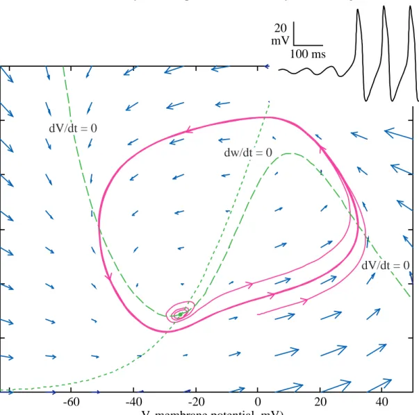
Another kind of behavior emerges for the MLE if external current is applied. Fig. 7 shows the phase plane and, in the insert at top right, the membrane potential versus time, when an external current (Iext) of 95 µA/cm

2

is applied.

The equilibrium point (green dot) still exists and is still a rest point of the system, but it is no longer attracting. One of the trajectories shown in magenta in Fig. 7 begins very close to the equilibrium point. As can be seen in the time waveform at upper right, the membrane potential oscillates with an increasing amplitude and then breaks into a large oscillation which is repeated exactly from cycle to cycle. This oscillation is called a limit cycle. The corresponding trajectory in the phase plane spirals around the equilibrium point with an increasing amplitude and then meets the limit cycle, which is the large closed curve in the plane. In this case, the limit cycle is the only stable element in the phase plane and the system will always end up in exactly the same limit cycle, regardless of the initial value. As an example, a second trajectory is shown in Fig. 7 beginning outside the limit cycle; this trajectory moves toward the limit cycle and joins it just after the peak membrane potential.

A limit cycle is a second feature of nonlinear systems which is not observed in linear systems. It is possible to have an oscillation like that shown in Fig. 7 in a linear system, but the amplitude of the oscillation is linearly proportional to the initial value. In a nonlinear system the limit cycles have a fixed amplitude, which is a characteristic of the system itself, and is not determined by the initial values. In a linear system, the oscillation can have any size, depending on the initial values. Of course a nonlinear system can have more than one limit cycle, but each limit cycle will be an isolated curve like the one shown in Fig. 7. By an isolated curve, we mean a closed curve which is not immediately adjacent to another limit cycle. Instead, trajectories slightly larger or slightly smaller than a stable limit cycle will spiral into the limit cycle, as in Fig. 7.

-60 -40 -20 0 20 40 V, membrane potential, mV) w , potassium activation 0 0.2 0.4 0.6 100 ms 20 mV dV/dt = 0 dw/dt = 0 dV/dt = 0

Fig. 7 Phase plane for the MLE with an external current Iext=95 µA/cm

2_{. Two trajectories are shown, one beginning}

near the equilibrium point (green dot at the intersection of the nullclines) and the second beginning at (0,0.14). The inset at top shows the time waveform for the trajectory beginning near the equilibrium point.

Linearization around equilibrium points

An important difference in the behavior of the MLEs between Figs. 5 and 7 is that the equilibrium point in Fig. 5 (with zero current) is attracting, i.e. trajectories flow into it, whereas the

one in Fig. 7 is not attracting, trajectories flow away from it. In fact, a great deal can be learned about the properties of nonlinear systems from their properties in the vicinity of equilibrium points. The approach is to compute a linear approximation to the nonlinear system in the vicinity of an equilibrium point. If the functions defining the time derivatives of the nonlinear system are sufficiently smooth, then in some small neighborhood of the equilibrium point, the linear approximation should behave like the nonlinear system.

Consider the nonlinear system at right. Xr is the system’s n-dimensional state vector. Eqn. 13 is exactly analogous to Eqns. 6 or 7, for n=4 or n=2, respectively. The functions fi(

r

X) can be expanded in a Taylor series around any point Xr₀; the first terms of such an expansion are shown in Eqn. 14. The notation X0i means the i

th

component of Xr₀. If Xr₀ is an equilibrium point, then f X_i(r₀)=0 for all i, from the definition of an equilibrium point, so that Eqn 14 simplifies to the linear equation in Eqn. 15. The matrix J of partial derivatives is called the Jacobian matrix of the system. Note that the Jacobian is a matrix of scalar constants.

r r r r r r r r ˙ ( ) ( ) ( ) ( ) ( ) ( ) ( ) X f X f X X X f X X X f X X X f X f X X X f X X X X X n X n n X X ≈ + − + − + ⋅⋅⋅ − + − + − + ⋅⋅⋅ 1 0 1 1 1 01 1 2 2 02 1 0 2 0 2 1 1 01 2 2 2 02 0 0 0 0 0 ∂ ∂ ∂ ∂ ∂ ∂ ∂ ∂ ∂ ∂ + ++ + ∂ ∂ ∂ ∂ ∂ ∂ ∂ ∂ f X X X f X f X X X f X X X f X X X n X n n n n X n X n n X n n 2 0 0 1 1 01 2 2 02 0 0 0 0 0 r r r r r ( ) ( ) ( ) ( ) ( ) − ⋅ ⋅ + − + − + ⋅⋅⋅ −                                 (14) r r r r r r r r r r ˙ X f X f X f X f X f X f X f X f X f X X X n X X X n X n X n X n n X ≈ ⋅⋅⋅ ⋅⋅⋅ ⋅ ⋅⋅⋅           ∂ ∂ ∂ ∂ ∂ ∂ ∂ ∂ ∂ ∂ ∂ ∂ ∂ ∂ ∂ ∂ ∂ ∂ 1 1 1 2 1 2 1 2 2 2 1 2 0 0 0 0 0 0 0 0 0               ⋅ − − ⋅ −                     = ( ) ( ) ( ) X X X X X X x n n 1 01 2 02 0 Jr (15) r r r r ˙ ˙ ˙ ˙ ( ) ( ) ( ) X X X X f X f X f X n n = ⋅ ⋅                             = ⋅ ⋅                             1 2 1 2 (13)

In the rightmost part of Eqn. 15 the vector xr=

[

]

equilibrium point Xr₀ is

r r r r r

˙x =Jx for x= −X X₀ and defined aboveJ

Question 7. Consider a second order system r˙x =J with initial value xr xr( )0 = xr₀. Show (by substitution) that the solutions of this equation take the form

r r r

x t( )=A eλ1t e +B eλ2t e

1 2 (16)

where λ1 and λ2 are the eigenvalues of J and er₁ and er₂ are the eigenvectors of J. Explain how to find the scalar constants A and B (hint: for λ1 ≠ λ2, the eigenvectors are linearly independent and form a basis set for the phase plane R2).

Question 8. Write the solutions of the system r˙x =J , xr xr( )0 = xr₀ for

J= J − − −           =           =           1 1 2 4 2 2 4 2 0 0

and xr and for the same with xr (17)

Question 9. Consider the system

˙ ˙ x y x x y x y = − + = − 3 (18)

Draw a phase plane for this system, including nullclines and equilibrium points. Compute the linearized system around the equilibrium points, including the eigenvalues.

Properties of systems linearized around an equilibrium point

The properties of the linearized system r˙x =J near the equilibrium point can be determinedxr

from the behavior of trajectories in the vicinity of the equilibrium point; it is sufficient to consider what happens if the state vector is moved slightly away from the equilibrium point, i.e. to consider an initial value problem for the system with initial value near the equilibrium point. The properties of such a system are determined by the eigenvalues. There are five important cases, listed below. The sketches at right show the nature of trajectories from initial values near the equilibrium point. In these sketches, the equilibrium point is at the origin of the plot and the axes are in the directions of the eigenvectors.

1. Stable node: λ₁ and λ₂ both real and negative. In this case the exponentials in Eqn. 16 both decay with time, so the trajectories move smoothly and exponentially toward the equilibrium point. Such an equilibrium point is an attractor for trajectories in its vicinity and may be an attractor for a large part of the phase plane.

2. Unstable node: λ₁ and λ₂ both real and positive. In this case the exponentials in Eqn. 16 both increase without bound, so the trajectories move away from the equilibrium point. The system is stable if placed exactly on such an equilibrium point, but any error will lead to a trajectory that moves away from the equilibrium point.

3. Stable and unstable spiral: λ₁ and λ₂ both complex; complex eigenvalues must occur in complex conjugate pairs. There are two cases, a stable spiral occurs when the eigenvalues have a negative real part and an unstable spiral occurs when the eigenvalues have a positive real part. The solutions in this case take the form AeRe[ ]λtcos(Im

[ ]

gives an oscillation at frequency Im[λ]/2π whose amplitude grows or shrinks according to the exponential multiplier exp(Re[λ]t). The sign of Re[λ] determines which. In the phase plane, such solutions will spiral around the equilibrium point, since there is a phase shift between the time waveforms along er₁ and er₂. The equilibrium point in Fig. 5 is a stable spiral (the exponential decay is faster than the period of the oscillation in this case, so the spiral is not seen; this case is very similar to a stable node) and Fig. 7 is an unstable spiral.

4. Saddle node: one real positive eigenvalue and one real negative eigenvalue. The two exponential terms in Eqn. 16 now behave oppositely. One decays exponentially, the other grows exponentially. In the figure at right, λ1 is negative, so the trajectories decay toward the equilibrium point along the direction of er₁; λ2 is positive, so the trajectories move away from the

equilibrium point along er₂. Most trajectories follow a hyperbolic path, as

sketched for the four trajectories shown with a single arrowhead. However, there are four trajectories which follow the directions of the eigenvectors er₁ and er₂ in the vicinity of the equilibrium point. These are indicated by the double arrowheads in the sketch. These trajectories are produced by initial conditions exactly on one of the eigenvectors, so that there is only one term in Eqn. 16.

The trajectories drawn above continue outside the range of the linearized system. The trajectories along the eigenvectors of a saddle node lead either to another equilibrium point or to a limit cycle (they cannot lead to infinity in a HH-type system; to see why, consider the behavior of the differential equations at 0, 1, EK and ENa see Question 12 below). In the larger nonlinear system,

they are called the unstable and stable manifolds, respectively, for the one leading away from and the one leading toward the saddle node. For the larger nonlinear system, they separate the trajectories of the system and can often serve as a true threshold, as described below.

e₂ e1 e2 stable unstable e1 e1 e2 e1 e2 e1 e2

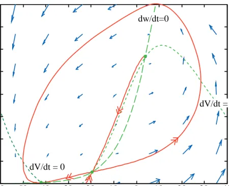
Figure 8 shows a phase plane for the MLE with the parameters of set #2. The components of the phase plane are marked as in Fig. 5. Note that there are now three e q u i l i b r i u m p o i n t s , marked by the green dots. The one near –42 mV is a stable node, the one near –20 mV is a saddle node, and the one near 4 mV is an unstable spiral. The stable and unstable manifolds are shown as the red trajectories with double arrowheads. These w e r e c o m p u t e d a s follows: for the unstable manifolds, the system was started with initial conditions near but not quite on the

saddle node. These trajectories were then computed directly in the usual way. One produced a subthreshold return to the stable node and the second an action potential which also returned to the stable node. The stable manifolds cannot be computed directly in this way, because there is no way to find an initial value on a stable manifold at a distance from the equilibrium point. Instead, the system was run in reverse time, i.e. the equations xr˙= −F xr r( ) and 0xr( )= xr₀ were solved. The only place that time appears in the differential equation is in the time derivative on the left hand side, so replacing t with –t changes the system only by reversing the sign of the time derivatives. With this change, all trajectories reverse direction and now the stable manifolds become unstable (i.e. lead away from the equilibrium point) and can be computed like any other trajectory.

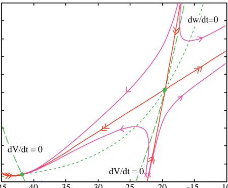
Figure 9 shows four trajectories in the vicinity of the saddle node. This plot shows the same phase plane as Fig. 8, except that the axis scale is magnified considerably. Only the stable node and the saddle node are shown (green dots), along with the nullclines (green) and manifolds (red). The magenta lines show four trajectories. Note how the trajectories follow the directions of the manifolds. This is typical of a saddle node. An important aspect of a saddle node is that trajectories cannot cross the manifolds, since the manifolds are themselves trajectories (the uniqueness theorem). There are two important implications of this fact:

1. The stable manifold running vertically downward from the saddle node acts as a true threshold for this system. This fact is apparent from Fig. 9. Consider trajectories from initial values (V1, w1) consisting of a depolarized membrane potential V1 and a resting value of the potassium

channel state w1. Such initial conditions lie along a line to the right of the resting potential. The

two initial conditions marked with x’s in Fig. 9 are on opposite sides of the stable manifold.

Fig. 8 Phase plane for the MLE with the parameters of set 2. All components are as for Fig. 5 except that the red lines are the stable and unstable manifolds. Note that there are now three equilibrium points (green dots).

-60 -50 -40 -30 -20 -10 0 10 20 30 40 V (membrane potential, mV) 0 0.1 0.2 0.3 0.4 w (potassium activation) dV/dt = 0 dw/dt=0 dV/dt = 0

One gives a subthreshold return of membrane potential to rest and one gives an action potential, by following the rightward directed unstable manifold. In this case, initial values to the left of the manifold, by however small an amount, give subthreshold responses and initial values to its right give action potentials. Thus crossing the manifold is the condition for threshold in this system. Furthermore, unlike the action potentials shown in Fig. 5 for parameter set #1, the peak membrane potential of the action potential does not depend on the initial condition, because the action potential trajectories fall very close to the unstable manifold.

2 You should be able to convince yourself, from Fig. 8 and Fig. 9, that there is no limit cycle in this system. Because the membrane potential cannot cross any of the manifolds, there is no way to construct a loop in this phase space that is consistent with the blue arrows.

In the discussion above, it was assumed that the system has two non-identical eigenvalues. When the eigenvalues are real and equal or when the eigenvalues are purely imaginary, then the linearized system turns out frequently not to be a good approximation to the nonlinear system, even

very close to the equilibrium point. This situation does not arise in practice, but care should be taken in cases where the eigenvalues are close to one of these degenerate cases. A more detailed discussion of this point is given in Strogatz, pp. 150-155.

Question 10. Repeat Question 8 for the following system.

J= − − −             =             1 5 1 4 2 2 0 and xr (19)

In case the eigenvalues of this system are complex; show that the solutions take the form

AeRe[ ]λ tcos( Im

[ ]

Fig. 9 Same phase plane as Fig. 8 shown magnified in the vicinity of the stable node and the saddle node. Green and red l i n e s a r e nullclines and manifolds as in Fig. 8. Magenta lines are trajectories from four initial values near the manifolds

-45 -40 -35 -30 -25 -20 -15 -10 Membrane potential, mV 0 0.01 0.02 0.03 0.04 w , potassium activation 0.05 dV/dt = 0 dV/dt = 0 dw/dt=0 xx

Question 11. Classify the equilibrium points for the system of Question 10 and sketch

trajectories in the phase plane for this system, based on the behavior of the equilibrium points. The chapter by Rinzel and Ermentrout (Koch and Segev, 1998, chapt. 7) contains several other interesting applications of phase-plane analysis to the MLE, including a very clear demonstration of how bursting can be added to this system using a physiologically realistic calcium-dependent potassium channel. In the following, phase plane analysis is applied to reduced HH systems in order to illustrate other applications of the method.

Necessary and sufficient conditions for a limit cycle

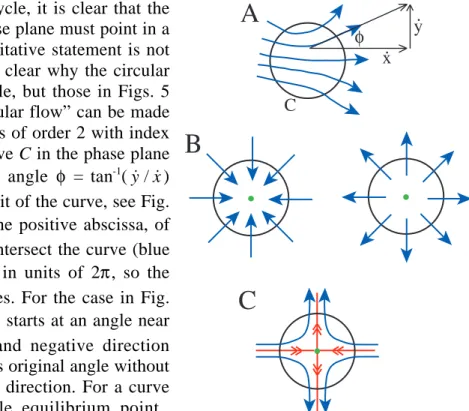
In order to have a limit cycle, it is clear that the direction of the arrows in the phase plane must point in a circular flow. However, this qualitative statement is not precise and it is not immediately clear why the circular flow in Fig. 7 allows a limit cycle, but those in Figs. 5 and 8 do not. The idea of a “circular flow” can be made slightly more rigorous for systems of order 2 with index theory. The index of a closed curve C in the phase plane is the cumulative change in the angle φ = tan-1

(y x˙ / ˙) through one counterclockwise orbit of the curve, see Fig. 10A. φ is the angle, relative to the positive abscissa, of the velocity vectors where they intersect the curve (blue arrows). The angle is measured in units of 2π, so the index takes on only integer values. For the case in Fig. 10A, the index is zero, because φ starts at an angle near 45˚, fluctuates in the positive and negative direction through the orbit, but returns to its original angle without making a complete turn in either direction. For a curve surrounding a stable or unstable equilibrium point (green dots in Fig. 10B), the index is +1 because in either case, the arrow makes one full counterclockwise revolution as the curve is orbited in the counterclockwise direction. Finally, for a saddle node, the index is –1, as in Fig. 1C.

The index of a curve in the phase plane has two important properties:

1. If C is deformed into another closed curve C’ without passing through an equilibrium point, as in Fig. 11, the index doesn’t change. This property can be understood as a consequence of the fact that we assume a continuously differentiable vector field for the phase-plane velocity. As a curve is deformed therefore, the index must also change in a continuous fashion, except at an equilibrium point. However, the index can only take on integer values, so it cannot change as the curve is deformed, except at equilibrium point.

y. x. C φ

Α

Β

C

Fig. 10. Closed curves (black circles) in a phase plane. Blue arrows are velocity vectors. A. No equilibrium point. B. Stable (left) and unstable equilibrium points (green dots). C Saddle node.

2. The index of a curve is equal to the sum of the indices around all the equilibrium points contained within the curve. This fact follows directly from property 1 and is illustrated in Fig. 11, which shows a curve C containing three equilibrium points (green dots). C is deformed into

C’ without crossing an equilibrium point, and therefore without changing its index. The index

of C’ is equal to the sum of the indices of the small circles around the equilibrium points plus the indices of the straight line segments. Each pair of straight line segments can be brought as close together as possible, so the index accumulated during transit in one direction along a line is exactly compensated by the transit in the other direction. This leaves only the indices of the three equilibrium points.

C

C’

A limit cycle is a closed curve in the phase plane. Its index must be +1, because the velocity vectors must be tangent to the limit cycle at every point (note that it doesn’t matter which direction the limit cycle runs, its index still must be +1). As a result, property 2 implies that a limit cycle must contain a number of equilibrium points whose indices sum to +1. That is, a limit cycle must contain an odd number of equilibrium points, with one more stable/unstable point than saddle node; for example two stable or unstable equilibrium points plus a saddle node satisfy the condition. Note that this is a necessary condition; a limit cycle does not necessarily exist in a phase plane which meets this requirement (as in Figs. 5 and 8). For the phase plane of Fig. 8, the manifolds of the saddle node are positioned in such a way that a limit cycle cannot exist, because there is no way to complete a loop around one or three equilibrium points without crossing one of the manifolds. Limit cycles can exist in systems with a saddle node, as in the example shown in Fig. 7.8 of Rinzel and Ermentrout (1998).

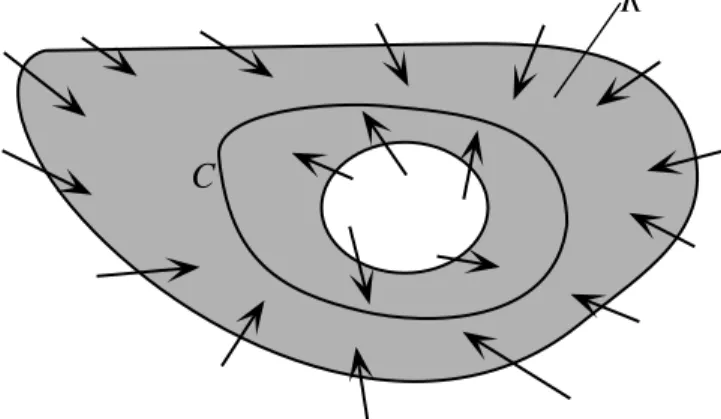
A sufficient condition for a limit cycle for order 2 systems (only) is provided by the Poincaré-Bendixson Theorem.

Theorem: Suppose that

1. R is a closed, bounded subset of the plane

(shaded at right);

2. dx dtr/ = f xr r( ) i s a c o n t i n u o u s l y differentiable vector field on an open set containing R;

3. R does not contain any equilibrium points; Fig. 11. Deforming

a closed curve C into a second curve C ’ without crossing an equilibrium point.

R

4. There exists a trajectory C that is confined in R, in the sense that it starts in R and stays in R for all time.

Then either C is a closed orbit (limit cycle) or it spirals toward a closed orbit as t→ ∞. In either case R contains a closed orbit.

This theorem imagines a situation in which the trajectory of the system is confined within a space R that is bounded on the outside, but also excludes a region in the inside, so that there can be an equilibrium point inside C to satisfy the index criterion. If conditions can be set up such that the velocity vectors point into the interior of R everywhere on both boundaries, then trajectories that are within R must stay there. Because there are no equilibrium points in R, the trajectory cannot approach a fixed position, which leaves only a limit cycle. The proof of this theorem is advanced; references to the proof are given by Strogatz (1994, p. 204).

Question 12. Argue that HH type systems have a natural outer boundary for R set by [0,1]

along the HH variable axis (e.g. w in the MLE) and by the equilibrium potentials for the ions along the V axis. Under what conditions can you show that an acceptable inner boundary can be set up (Hint, consider the situation in Fig. 7)?

The Poincaré-Bendixson theorem can be applied to show that a limit cycle must exist in the case of Fig. 7, for example.

Threshold behavior from the V-m reduced HH system

The following discussion is based on Fitzhugh’s (1960) analysis of the HH system in reduced form. Consider first the conditions for threshold when a cell is depolarized by a brief current injection. As in Figs. 5 and 9, this situation is modeled by using an initial condition in which membrane potential is displaced away from the resting equilibrium point without changing the other state variables. Figure 3 shows that the initial event in response to such a stimulus is a rapid increase in m and V, with changes in h and n that occur more slowly. Thus it seems reasonable to replace the full HH system with a reduced system consisting only of two state variables, V and m and hold h and n constant at their resting values. Then the system becomes

CdV dt I G m h V V E G n V V E G V E dm dt m V m V ext Na R Na K R K L L m = − − − − − − = − ∞ ∞ ∞ 3 4 ( )( ) ( )( ) ( ) ( ) ( ) τ (21)

where VR means the membrane potential before the application of current, for example the resting

potential. Note that h and n are now held constant at their steady-state values at VR.

Consider first the behavior of the reduced system starting from the resting potential, -60 mV. Figure 12 shows a phase plane for the (V, m) system with h=h_∞(-60)=0.596 and n=n_∞(-60)=0.318. The conventions and color code are the same as for phase planes in previous figures. There are three equilibrium points (green dots) in this system, a stable point at the resting potential (-60 mV, labeled r), a saddle node just above the resting potential (-57.3 mV, labeled s) and another stable point at depolarized potentials (+53.9 mV, not labeled). The manifolds associated with the saddle

node are drawn in red. The expanded view at right shows the structure of the phase plane near the resting potential and the saddle node.

-100 -800 -60 -40 -20 0 20 40 60 0.2 0.4 0.6 0.8 1 Membrane potential, mV m dm/dt=0 dV/dt=0 r -60 -59 -58 -57 -56 0.05 0.06 0.07 0.08 0.09 Membrane potential, mV dm/dt=0 dV/dt=0 r s s

The stable manifold that extends downward from the saddle node acts as a threshold separatrix, just as it did for the MLE system in Figs. 8 and 9. Trajectories beginning at membrane potentials just to the left of and just to the right of this threshold (not shown) follow the unstable manifolds, ending at one or the other stable equilibrium potential. The full system behaves similarly, in that it has a sharp threshold in the same region. Thus, it seems reasonable to study threshold behavior in the full model by assuming that threshold corresponds to crossing the stable manifold in the reduced system. The similarity is qualitative, however, in that the threshold for membrane potential displacement predicted by the reduced model (-56.75 mV) is somewhat different from the threshold of the full model (-53.44 mV).

The behavior of the reduced system is compared with the full system in Fig. 13, which shows two trajectories in the (V, m) phase plane. Both trajectories are from initial values just above the relevant threshold; the one from the reduced system (V-m sys, black) follows the unstable manifold to the large-depolarization equilibrium point, whereas the other (H H , magenta) follows a slightly different path to depolarized potentials and then returns to the equilibrium point. Note that the magenta trajectory is not the actual trajectory of the system, which is a curve in 4-dimensional space. Instead it is a projection of that trajectory on the V-m plane. Of course, it is not expected that the reduced system should produce a full action potential, because to do so requires either h or n or both. The purpose of the reduced system is only to analyze the

Fig. 12. Phase plane for the reduced system with V and m as state variables. Expanded view shown at right.

Fig. 13. Comparison of trajectories of the reduced system (black) and the full system (magenta) on the V-m phase plane. Both trajectories begin just above voltage-displacement threshold. s -100 -800 -60 -40 -20 0 20 40 60 0.2 0.4 0.6 0.8 1 Membrane potential, mV m r V-m sys. HH

conditions for threshold, under the control of V and m.

Question 13. The magenta trajectory in Fig. 13 is inconsistent with the blue arrows. Explain

why.

The behavior of the reduced system depends on the values chosen for the state variables that are held constant. Figure 14 shows the effect of the value of h on the threshold. Shown is the m nullcline (long dashes) and the V nullcline (short dashes) for two values of h, as labeled. The effect of h on the V nullcline can be seen from the equation for the V nullcline,

dV dt m V I G n V V E G V E G h V V E V ext K R K L L Na R Na = ⇒ = − − − − −       ∞ ∞ 0 4 1 3 ( ) ( )( ) ( ) ( )( ) / (22) which is obtained by solving Eqn. 21 for m with

dV/dt=0. As h decreases the V nullcline moves vertically

upward. The result is to move the saddle node to the right along the m nullcline. As the saddle moves, the downward-pointing stable manifold is dragged along. Because that manifold is the threshold separatrix, the effect is to increase the threshold. The horizontal black line shows where the thresholds are, at its intersection with the stable manifolds, and shows clearly the increase in threshold as h decreases. This behavior in the phase p l a n e c o r r e s p o n d s

physiologically to the fact that as h decreases, sodium channels are inactivated and therefore unavailable to participate in action potentials. The full model behaves qualitatively similarly, with the threshold going from –53.44 mV for h(0)=.596 to–38.07 mV for h(0)=0.1.

Question 14. It is apparent from Fig. 12 that the near-threshold intersection region of the V

and m nullclines is very small. Argue from Eqn. 22 that by injecting positive current it is possible to eliminate the intersection of the nullclines near the resting potential, so that the only equilibrium point in the V-m plane is the one near +50 mV. (Hint: what is the sign of V-ENa?) How will the

reduced system behave in this case? What does the reduced system predict about the full system in this situation?

Fig. 14. Effect of varying h on the reduced system in the V-m phase plane. 0.596 is the value of h at the HH resting potential Note the change in the stable

-1000 -80 -60 -40 -20 0 20 40 60 0.2 0.4 0.6 0.8 1 Membrane potential, mV h=0.596 h=0.1 dm/dt=0 m

The V-m reduced system provides insight into the phenomenon of anode-break excitation, seen in both the squid giant axon and the HH model. Figure 15 shows the phenomenon, in the full model, at upper left. The membrane is hyperpolarized by a –2.8 µA/cm2

current injection over the time period 0 to 40 ms (the heavy bar on the abscissa). When the current is turned off, the membrane potential returns toward rest, but then overshoots the rest potential and fires an action potential. Qualitatively, the anode-break effect can be explained by the fact that h increases and n decreases during the maintained current injection, so that the membrane is more excitable at the end of the current (time tend); the increase in h means more sodium channels are available for activation

and the decrease in n means that fewer potassium channels are open to stabilize the membrane.

-80 -40 0 40 Membrane pot., mV 0 20 40 60 0 0.2 0.4 0.6 0.8 1 HH variables Milliseconds h n m t_end -1000 -80 -60 -40 -20 0 20 40 60 0.2 0.4 0.6 0.8 1 -650 -60 -55 -50 -45 -40 -35 0.1 0.2 Membrane potential, mV m dm/dt=0 dV/dt=0 m dm/dt=0 dV/dt=0

The phase planes at right in Fig. 15 show the reduced V-m system with n and h set at their values just at the end of the hyperpolarization, i.e. at time tend in Fig. 15 (n is 0.272 instead of the

resting value of 0.318 and h is 0.695 instead of its resting value of 0.596). The effect of reducing n

Fig. 15. Anode-break excitation. Top left shows time waveforms of membrane potential and the HH variables for the full HH model in response to a 40 ms long –2.8 µA/cm2 _current

injection (heavy black bar). At right are V-m phase planes for the instant just after the current is

and increasing h is to move the dV/dt nullcline downward, eliminating the intersection of the nullclines near the rest potential. As a result, there is now no stable equilibrium point in the reduced system, except near +50 mV. The flows in the vicinity of rest potential are shown at lower right in Fig. 15. The magenta line shows the trajectory of the reduced system through this region from an initial condition at the values of V and m at the end of the hyperpolarization. The explanation for the anode-break spike, in terms of the phase plane analysis, is that the stable equilibrium point at the resting potential is abolished by the changes in n and h so the system undergoes a rapid depolarization which leads to an action potential in the full system.

Bifurcation theory illustrated with the V-n reduced HH system

A reduced system similar to the MLE can be constructed from the HH equations by eliminating m and h as state variables, leaving V and n. This approach was taken by Cannon and collaborators (1993) in a model of certain muscle disorders linked to loss of inactivation in the sodium channels in the muscle. The first assumption is that the time constant for m is fast, so that m can be approximated by m_∞(V). The second assumption is to set h to zero, which is a crude approximation of the situation during the repolarization phase of the action potential, after about 2.5 ms in Fig. 3, when most sodium channels are inactivated. The muscle disorders studied by Cannon et al. show a loss of repolarization, so this phase of the action potential was of primary interest in their study. The model assumes that some sodium channels, a fraction f, have lost their inactivation gates, so that their conductance is gated only by the activation gate m. The resulting model contains only two state variables and resembles the MLE:

dV dt C I G f m V V E G n V E G V E dn dt n V n V ext Na Na K K L L n =

[

]

Note that the sodium term assumes that f of the sodium channels do not inactivate and the remainder are permanently inactivated. The functional form of m_∞(V) and

n_∞(V) used by Cannon et al. are the same as in the original HH model, but the parameters are different. The parameters are listed in the appendix. (Note that with these parameters, the behavior of the model is qualitatively the same as published, but the quantitative behavior, i.e. values of f at the bifurcation points, is slightly different; presumably this difference reflects some difference in parameter values actually used by Cannon et al. versus the ones gleaned from their paper.)

The reduced n-V model produces action potentials that are qualitatively similar to the full HH model. Figure 16 shows a comparison of the action potential and n(t) waveforms between the full model (solid lines) and the reduced model (dashed lines) with

f=0.025.

Fig. 16. Comparison of the membrane potential (top) and n(t) waveforms between the full (dashed) and reduced (solid) Cannon models (Fig. 9A of Cannon et al, 1998)

The phase-plane of the reduced model is shown in Fig. 17A for a range of values of f. The V nullcline is shown by the solid lines. As in the MLE, the V nullcline has two legs, a negative slope portion below –80 mV which does not vary as f varies, and a convex upward portion between about –60 and +40 mV which is quite sensitive to f. The n nullcline is shown by the dashed line. As before, this nullcline is a plot of n_∞(V) and does not depend on f. There are three equilibrium points in the system, indicated by the symbols. One, the rest potential (r.p.), is stable, and remains near –85 mV for all values of f . A second equilibrium point is near –60 mV (open triangles); this point moves with the V nullcline as f changes. It is a saddle node with a stable manifold that serves as a threshold separatrix, as in Fig. 8. The manifolds are not shown, but the stable threshold manifold follows very closely the

dV/dt=0 nullcline in the

downward direction. A third equilibrium point is near and

above –40 mV. It can be a stable (filled squares) or unstable (unfilled squares) spiral, depending on

f.

As f decreases, the upper two equilibrium points move toward one another along the dn/dt=0 nullcline until they coalesce into a single point for f =0.013 and disappear for smaller values. Note that there is only one equilibrium point, the r.p., for the smallest value of f shown in Fig. 17A.

The bifurcation diagram in Fig. 17B summarizes the behavior of the system on a plot of the membrane potential at the equilibrium points (ordinate) versus the value of f, which is the bifurcation parameter in this case. In nonlinear dynamics, a bifurcation means a sudden change in the qualitative behavior of a system with a small change in some parameter. The line marked stable

node shows the membrane potential at the r.p., which does not change with f; this point remains Fig. 17. A. Phase plane for the reduced Cannon et al. model with f varying from 0.01 to 0.1. Shown are nullclines; only the dV/dt=0 nullcline varies with f. Symbols marking equilibrium points vary in shape according to eq. point type. r.p. is equilibrium point at resting potential. B. Bifurcation diagram for this system. (modified from Fig. 10 of Cannon et al., 1998.)

stable across the range of f. The sidewise parabola-like curve at higher membrane potentials plots the positions of the other two equilibrium points. The lower branch of this curve, marked unstable

saddle, plots the potential of the saddle node; the upper branch plots the potential of the third

equilibrium point, which is either unstable or stable. The coalescence and vanishing of the upper two equilibrium points is clearly shown as the left–hand end of this plot at f=0.013. The disappearance of the upper two equilibrium points is called a saddle-node bifurcation; such a bifurcation often has interesting consequences for systems. In this case, the effects are subtle, and a more interesting example is shown in Fig. 7.5 of Rinzel and Ermentrout, 1998. Solid lines show stable equilibrium points and dashed lines show unstable points, including saddles. The transition from unstable to stable at f=0.048 is shown on the upper limb for the third equilibrium point.

The model shows a range of behaviors as f varies. For f very small, there is only one equilibrium point at the resting potential and all trajectories decay to the resting potential, which is globally attracting. The model behavior is similar to the MLE shown in Fig. 5.

For larger values of f, three equilibrium points exist; for f between 0.013 and 0.048, the upper one (near –40 mV) is unstable (open squares in Fig. 17A, dashed line in Fig. 17B). The saddle node’s manifolds are positioned as in Fig. 8; the stable manifold provides a threshold, as it did for the MLE. The equilibrium point at the resting potential is still globally attracting. It is possible to convince yourself of this last point without doing simulations. First, the equilibrium point at r.p. is the only stable equilibrium point in the phase plane. Second, there cannot be a limit cycle because, from index theory, it would have to cross one of the manifolds of the saddle node, as for Fig. 8. Finally, the system cannot cross the outer boundary set by the equilibrium potentials and [0,1] along the n dimension, as argued in Question 12. Thus there is no stable state of the system other than the equilibrium point.

At f=0.048, the upper equilibrium point becomes a stable spiral; the eigenvalues of this equilibrium point are a complex conjugate pair and their real part changes from positive to negative at f=0.048. When the upper equilibrium point becomes stable, the behavior of the system changes in an important fashion, which was the main subject of the paper by Cannon et al. because it resembles the pathophysiology of the muscle disorder they were studying. Over a narrow range of f, there are two stable states of the system with the structure shown in Fig. 18. The phase plane at left in Fig. 18 shows three equilibrium points (green dots), as in Fig. 17A. The nullclines and the manifolds of the saddle are shown in green and red as before. Trajectories from three points in the phase plane are plotted by the magenta, blue and brown curves. The corresponding time waveforms are shown in the inset. The blue and brown trajectories correspond to action potentials that end up at the r.p. equilibrium point, as before. However, the magenta trajectory produces and action potential that does not repolarize to rest; instead, it oscillates around the third, now stable, equilibrium point (at –32 mV), and eventually comes to rest there. The failure to repolarize, of course, occurs because the sodium channels are not inactivating, so that the membrane potential is maintained in a depolarized state by steady-state sodium currents. This can only occur when the fraction of non-inactivating sodium channels exceeds about 0.048, i.e. at the bifurcation point where the third equilibrium point becomes stable.

The phase plane is now divided into two regions: the area inside the curve plotted with the dashed black line in Fig. 18 is the basin of attraction of the third equilibrium point. All trajectories that begin inside this curve, like the magenta one, end up at the third equilibrium point. The rest of

the phase plane is the basin of attraction of the resting equilibrium point, as before. Note that the upper stable manifold of the saddle node (red manifold extending upward from the saddle node) does not originate at the third equilibrium point, as it does at lower values of f (in exactly the same way as in Fig. 8). It cannot do so, because that equilibrium point is now stable. Instead, it originates in an unstable limit cycle corresponding to the black dashed curve.

-1000 -60 -20 20 0.2 0.4 0.6 0.8 1 Membrane potential, mV x x x Potassium activation, n -60 -40 -20 0 0.5 0.6 0.7 dn/dt=0 dV/dt=0 0 10 20 30 ms 0 -40 -80 mV

Up to now, only stable limit cycles have been considered. Stable limit cycles are curves into which other trajectories move, as in Fig. 7. It is also possible for limit cycles to be unstable, in which case trajectories diverge from them. Unstable limit cycles can be discovered by the trick of reversing time in the simulation, as discussed in connection with Fig. 8. With reversed time, all trajectories reverse direction, stable elements become unstable and vice-versa. The unstable limit cycle in Fig. 18 (dashed black curve) was plotted in this way. This limit cycle, or unstable periodic orbit, serves as a separator between the basins of attraction of the r.p. and the third equilibrium point.

Question 15. Sketch the phase plane of Fig. 18 for the negative time system. In particular,

show what you think will happen to trajectories beginning at the three initial values marked with x’s (i.e. the initial values of the magenta, blue, and brown trajectories).

Fig. 18. Phase plane for the reduced model of Cannon et al. with f=0.062 and the parameters given in the appendix. The color code is the same as in previous figures; trajectories from three initial values (x’s) are shown in magenta, blue, and brown. The brown trajectory follows the unstable manifold of the saddle from the vicinity of the third equilibrium point to the r.p. and cannot be seen because it is occluded by the manifold. The plot at right is an expanded view of the phase plane near the third equilibrium point. The trajectories are very crowded just above this equilibrium point, but the magenta curve is inside the boundary set by the dashed black curve and the blue, red, and brown trajectories are outside it (the brown trajectory is hidden behind the red manifold). The inset at top center shows the time waveforms corresponding to the three trajectories, using the same color code. Note that Cannon et al. show the same behavior (their Fig. 11) for f=0.055.