Designing coordination contracts to support
efficient flow-scheduling in pork chain
Jarkko K. Niemi
MTT Agrifood Research Finland, Economic Research, Kampusranta 9, FI-60320 Seinäjoki, Finland
Revised version, August 2012
Selected Paper prepared for presentation at the Agricultural & Applied Economics Association’s 2012 AAEA Annual Meeting, Seattle, Washington, August 12-14, 2012
Copyright 2012 by Jarkko K. Niemi. All rights reserved. Readers may make verbatim copies of this document for non-commercial purposes by any means, provided that this copyright
Designing coordination contracts to support efficient flow-scheduling in pork chain
Jarkko K. Niemi, MTT Agrifood Research Finland, Economic Research
Abstract
Risk management and efficient, well coordinated, flow-scheduling have an increasingly important role in the competitive pork production networks. Changes in input and output prices have resulted in distortions in the Finnish pig markets during the last years. The goal of this study is to estimate how different price or quantity-fixing contracts affect the values of pig and sow space unit under price risk. The values are estimated with two stochastic dynamic programming models. The results suggest that a contract which is able to control both the pattern of changes in piglet prices and the option to suspend production temporarily has a value and it can help to improve the competitiveness of the pig sector. However, it is feasible to have incentives towards the contract commitment only when market situation is favourable for the commitment.
Keywords: Pigmeat, piglet, price feed, contract, market distortions
1. Introduction
Risk management and efficient, well coordinated, flow scheduling have an increasingly important role in the competitive pork production networks. There are at least two reasons for this. Firstly, individual producers can improve their efficiency in a manner similar to efficient capital markets. While searching for efficiency gains through increasing specialization and size of their production, they also enhance risk management through innovative contract coordination mechanisms and investment portfolios such as diversified ownership structures. If the contract coordination is successful, the network can be split into vertically coordinated, highly specialized, efficient and capital intensive firms. In the livestock sector specialization allows to gain economies of scale in
production processes even in small or moderate size firms, since the operations are often regulated by environmental regulations which are dependent on firm size.
Secondly, the volatility of agricultural commodity market has increased in the recent years, and it may increase also in the future as public market interventions are gradually withdrawn and climate change increases the likelihood for adverse supply shocks in the sector. It may increase also in the future as public market interventions are gradually withdrawn and climate change increases the likelihood for adverse supply shocks in the sector (cf. OECD-FAO 2010). Hence, increasing price volatility can further increase producer incentives to enter in risk-reducing and price-fixing coordination contracts. As an example, pig markets are rather volatile. According to the Finnish Farm Accountancy Data Network results (MTT, 2012), the coefficient of variation (CV) of entrepreneur’s profit was 26% during the period from 2000 to 2011(e), and CV of parameter profitability ratio was over 30%. Since these values reflect industry’s average, they are heavily influence by price volatility. At the enterprise level the volatility of profits and revenues can be even higher, because there biological parameters can also vary a lot. Over the past few years, changes in feed grain and soybean meal prices have caused fairly large fluctuation s in economic result of pig farms. During 2000 to 2011, CV’s for monthly feed, piglet and pigmeat prices (Statistic Finland, 2012) were 11%, 15% and 7%, whereas during 2007-2011 they were 9%, 3% and 4%, respectively. The increased wedge between input and output prices, as associated with price volatility, has resulted in distortions in the Finnish piglet market over the past few years. As meat prices haven’t been increasing at the same rate as feed prices, some finishing farms have found it optimal to pause production temporarily and continue production after the markets have recovered. This has resulted in overstocking in farrowing units.
If the chain involves significant amount of interruptions in the flow scheduling, the efficiency of the network could be improved with a contract where finishing farms are committed to purchase certain, predetermined amount of weaners to maximize the returns for the whole supply chain. Producers who give away the option to suspend production and commit to produce at full capacity, even if meat prices plunge, should demand a compensation for the commitment. Coordination contracts which have the power to decrease price volatility and which affect the optimal investment thresholds can help to improve the competitiveness of the pork supply networks particularly through the structural development of the pork sector. If a coordination contract is successful in decreasing the risk, it narrows the wedge required between the input and output prices and triggers new investments along the contract-specific production and marketing systems (Pietola and Uusitalo 2001, 2002). The contract is important also as to ensure the continuous availability of meat to be processed and to increase the usage rate of production capacity. Various combinations of procurement arrangements have been found to improve short-term processor plant performance relative to the situations in which the plant uses only cash/spot markets to purchase all of its slaugter pigs (Vukina et al. 2009). The use of contracts can vary by situation. Zheng et al. (2008) found that producers using production contracts were more risk averse than those using the spot markets or marketing contracts. Moreover, Dubois and Vukina (2009) found that producers with higher risk aversion had lower outside opportunities and hence lower reservation utilities.
When designing the contract, it is important to understand how offered price or quantity-fixing contracts affect the farm business. Widely adopted approach to account for uncertainty in agricultural investment problems is to augment the standard net present value models by real options (Dixit and Pindyck 1994). The real options can be used to investigate the value of investment when producer has the option to adjust his/her decisions according to information that is available each moment as compared to waiting for more market information that arrives with the
passage of time (e.g. McDonald and Siegel 1986). The producer can have options such as an option to defer the investment; to temporarily suspend production and restart it when revenues increase again; and to abandon the investment, for instance, by renting out or selling the facility already before the invested good has been exhausted (Trigeorgis 1996). Odening et al. (2005) conclude that the investment trigger, taking into account the value of waiting in an uncertain environment, can be considerably higher compared to classical investment criteria such as the net present value, which may contribute to the reluctancy to invest in pig production. Hinrichs et al. (2005) found that uncertainty and flexibility widen the range of economic returns where inaction is the optimal choice for the producer. That is, a higher return is required to investment in new production capacity and a lower return is required to disinvestment that would be required in the absence of flexibility.
Livestock markets are often criticized for price rigidity and that changes in input prices are transmitted sluggishly to meat prices. As livestock production process takes time, it can be costly for producers to suspend production unless the fattening pig stock is ready to be marketed. One implication of this is that if producers are faced by a strong market shock resulting in falling meat prices while input prices remain unchanged, may suffer large losses (cf. Niemi and Lehtonen 2010). Hence, it is important to consider also how the correlation between input and output prices can impact the value of contract.
Carrying out an irreversible investment reduces individual producers’ options to adjust in price shocks. However, if the marketing contract is loose enough even then an individual farm specialized in pig fattening, may have an option to suspend production if its revenues fall below the variable costs and, thereafter restart production again once revenues have recovered. Retaining such an option may be valuable for an individual fattening unit but costly for the whole pork production chain (Pietola and Wang 2000). The costs are increased because the suspension option requires
excess capacity elsewhere in fattening stage, or causes severe distortions in the flow scheduling of piglets. Interruptions at fattening stage imply problems for piglet producers in finding a buyer for their animals and may require maintaining over-due piglets on the farm. The problem is further exacerbated if the stocking rates increase to the extent that animal welfare is compromised.
If the chain involves significant amount of interruptions in the flow scheduling, the efficiency of the network could be improved with a contract where fattening farms are committed to purchase certain, predetermined amount of piglets to maximize the returns for the whole supply chain. Producers who give away the option to suspend production and commit to produce at full capacity, even if meat prices plunge, should demand a compensation for the commitment. Pietola and Wang (2004) suggests that the option to suspend production temporarily has substantial value for an individual fattening farm. Hence, an optimal contact that is fixing the quantity flow at full capacity through the supply chain accounts for this value. Pietola and Wang (2004) approach was based on fixed input-output enterprise budgets. In this study we allow the growers to adjust also through feeding and the timing of slaughtering rather than suspending their production. Another closely related approach is by Burt (1965, 1993) who has analysed the decisions of finishing farms under risk using dynamic programming.
The goal and contribution of this study is to estimate how different price or quantity fixing contracts affect the value of finishing pig space unit in a more realistic decision setting framework than in previous studies, the value of sow space, and the value of these together. The value of finishing pig space unit is estimated with a stochastic dynamic programming algorithm which is based on the integration of two models. The first model maximises the value of a finishing pig space unit by using four decision variables, i.e. feeding, the timing of slaughter, and production breaks, i.e. the decision to purchase weaners. The input-output ratios are endogenous and the option to suspend
production temporarily is taken into account in the model. This stochastic decision problem does not have a closed form solution and it is therefore solved numerically with a stochastic dynamic programming algorithm. The second model is optimising the supply of weaners from a farrowing farm with a stochastic dynamic programming model. Results from two models are integrated and the efficiency of a coordination contract is analysed as to maximise return on the production chain.
2. Models
Dynamic programming has been used to optimise both piglet production management decisions (e.g. Jalvingh ym. 1992; Huirne ym. 1993; Kristensen ja Søllested 2004; Plá 2007) and finishing pig production (e.g. Glen 1983, Burt 1993, Niemi 2006). The method is well suited to solve optimisation problems which are sequential or are subject to uncertainty about future events. Uncertainty can be taken into account when optimising decisions and decision-maker can respond to observed events. The approach used in the studies mentioned above could be extended to the production chain such that producers optimise not only their own production, but also take into account the behaviour of producers in other production stages. In this study, we assume examine an individual farrowing farm and an individual finishing farm and optional contracts that they can make when piglet, feed and input prices are stochastic. We consider different aspects of a contract that both farms can choose:
1) Status quo, where the farrowing farm sells piglets to the cash market and the finishing farm buys the piglets at from the market at currently valid market price. The finishing farm has the option to pause production temporarily if it is considered optimal (“outside option”). 2) Quantity-fixing contract such that the farrowing farm and the finishing farm agree to trade
Both are committed to produce at the full capacity, i.e. the finishing farm gives up the option to pause production temporarily.
3) Quantity-and-price-fixing contract such that the farrowing farm and the finishing farm agree to trade piglets, but changes in the price of piglet are similar to the changes in the price of pigmeat. Both are committed to produce at the full capacity, i.e. the finishing farm gives up the option to pause production temporarily.
This paper mainly focuses on comparing quantity-and-price-fixing contract (3) to status quo (1). The farrowing farm, once decided to start production, has only limited options to alter production because it is costly to cease production. It therefore doesn’t have to option to pause production temporarily even if the finishing farm would have such an option. However, the farrowing farm may adjust the replacement rate of sows in order to maximise returns on sow space. Piglet production is modelled as an infinite-horizon and finishing pig production for a finite horizon optimisation problem because the analysis is computationally more efficient this way. The results are converted to per animal basis to allow the comparisons between two models.
Althoughtwe don¨t explicitly consider risk aversion,in one-period returns, it is implicitly included in the model.This is due to option values that the model evaluates each period.
2.1.A model for a farrowing farm
Piglet production is modelled with a stochastic dynamic programming model, which has some similarities with the model presented by Kristensen ja Søllested (2004). A major difference is that in this paper prices are considered stochastic. The model does not commit to specific capacity
constraints of pig production. It optimises production on the condition that sufficient production capacity is allocated to each production stage. Hence, the outcome is return on investment in specific production technology. Cost of capacity (i.e. fixed costs) is included in the model as time-constant factor, because fixed costs are needed to make different production stages consistent when evaluating the effects of genetic and managerial improvements on the production cost of pig meat.
The objective of a farrowing farm is to maximise net returns to sow space unit by optimising the timing of replacement regarding sows. The model characterises the most important events related to sow’s and piglet’s productive life. Decisions rules are solved and corresponding returns simulated by the state of nature, which represents observable characteristics of a sow; i.e. parity and piglet yield in the previous parity. In addition, time index is used to characterise the stage length and a large number of parameters are used to characterise sow’s productivity at a given state of nature. Exact yield and prices in the future are however unknown a priori. By contrast, the mean and variance of both biological and market parameters are known.
The Bellmann equation (1957) of the sow herd problem is of the form:
(1) (xt) max t,sow(xt, t) ( t 1(xt 1)) t u t R u E V V , t=1,…, ∞ and where } , , , ,
{xt,piglet xt,feed xt,meat xt,parity xt,litter
t
x
subject to: xt 1,piglet g1(xt,piglet,xt,feed,xt,meat)
) , ,
( ,piglet ,feed ,meat 2 feed , 1 t t t t g x x x x ) , ,
( ,piglet ,feed ,meat 3 meat , 1 t t t t g x x x x ) , , , ( ,parity ,litter 4 litter , 1 t t t y t g x x u x ) ), , ( , , ,
( ,parity ,litter involuntary ,parity ,litter infertile 5 parity , 1 t t t t t t g x x u x x x
t
x and V (x ) are given,
where t is time index; xt is the state vector where xt,piglet,xt,feed,xt,meat,xt,parity and xt,litter represent state variables piglet price, feed price, pigmeat, currently observed parity and currently observed litter size (i.e. piglet yield in the current parity) in period t,respectively; Vt(xt) is the value function (i.e. maximised value of a capacity unit as a function of the state variable) in time period t;
sow ,
t
R is
one-period returns function for time period t; ut is the control variable; β is discount factor; E(.) is expectations operator applied on the term inside brackets; Vt 1(xt 1) is value function at period t+1; g’s are transition equations governing the evolution of state variables over time as functions of state variables and control policy; π’s are probabilities for events indicated by subscript, δ segregates to subparameters and describes time interval required for a sow to reach subsequent production stage, and y and εp are vectors indicating variation of movement related to the state variable in the subscript. The transition equations for litter size and parity have autonomous part which realises deterministically, controllable part which depends on the control variable, and random part, which is exogenous, whereas transition equations for prices are exogenous to the producers except for the part which is dependent on the choice of contract type.
The control variable can have two values {0,1}, where 0 refers to not replacing the current sow with a primiparous sow after the current parity, and 1 refers to the opposite case. However, note that there is a parity and litter size-dependent probability (xt,parity,xt,litter) that the sow must be replace
because of an exogenously given reason.
Pigmeat price is directly irrelevant to the farrowing farm in the current situation, but it is introduced also into the farrowing farm model model to ensure consistency between the models and because pigmeat price is relevant in scenarios where piglet prices are governed through the movement of pigmeat prices. The transition equations for piglet, feed and pigmeat prices are given in section 2.3, whereas transition equations for parity and litter size are characterised in this section.
Movement of state variables over time is governed by transition equations g as follows:
(2) 1 if 1 0 if ) , ( )) , ( 1 )( 1
( ,parity ,parity ,litter ,parity ,litter parity , 1 t t t t t t t t u u x x x x x x , (3) 1 if 0 if ) , ( 1 ( ) , ( )( ) , ( ( prim prim litter , parity , litter , parity , piglet parity , piglet , 1 piglet , piglet , 1 t t t t t t t t t t u u x x x x x x f x x ,
where f1 (xt,piglet,xt,parity) represents the average change in litter size between successive parities to
the extent that is can be forecast by current litter size, parity number and other predetermined factors, piglet is unpredictable random change (i.i.d.) in litter size between successive parities, and change and prim is distribution of litter size for primiparious sows. It is assumed that the variance of prim and pigletare known, and that primhas a positive mean and piglet has zero mean. There is a parity and litter size-dependent probability (xt,parity,xt,litter) that the sow must be replaced because
of an exogenously given reason, such as disease, death or animal health problem. In the farrowing farm model decisions are taken once per farrowing, i.e. when it is time to replace or reinseminate the sow. The time interval between successive decisions is set constant.
Litter size transition equations and biological aspects related to farrowing farm are parametrised by using data obtained from Faba breeding, a former animal breeding co-operative in Finland. There are data about 12 197 sows born in 2002. Piglet growth, survival and feed intake data are from MTT Agrifood Research Finland’s experimental station, because other data do not fully cover these aspects.
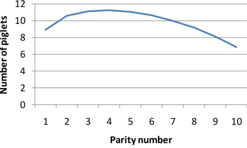
Figure 1 represents the development of the number of piglets born as a function of parity number on average. Should current litter size deviate from the average figure then, based on our data, only little more than 20% of this deviation is on average repeated in the next farrowing. As an example of a typical case, a sow can produce on average 11.6 piglets per farrowing. In addition, a varying number of piglets are stillborn or die after their birth. The correlation between different biological parameters of the sow was based on data obtained from MTT and results reported by Serenius et al. (2004). On average, almost 19% of piglets are lost either as stillborn piglets or due to postnatal piglet mortality. This leaves on average 9.5 piglets to be weaned of which 3 % are lost after weaning so that only 9.2 piglets per farrowing would be marketed. However, this is just an average value simulated using the model parameters, because the parameters of the sow are stochastic and dynamic.
0
2
4
6
8
10
12
1
2
3
4
5
6
7
8
9
10
N
u
m
b
e
r
o
f p
igl
e
ts
Parity number
Figure 1. The average number of piglets born as a function of partiy number.
Economic parameters and one-period returns
In the recursive structure, the cash flow of farrowing farm is described by one-period returns which are obtained over time and separately for each time period. One-period returns depend on
the state of nature, policy chosen and economic parameters. These returns include returns from selling the piglets, the costs of feeds, insemination, replacements sows, labour and veterinary services. The total costs of producing piglets are accounted for, but because some of these costs are fixed costs, they don’t affect the model’s solution. Table 1 characterises the costs of production at November 2011 prices. Please note that feed costs depend on piglet yield (values in Table 1 are standardised for a 9.5 piglets litter). Feed and piglet price are assumed stochastic, because the remaining price parameters seem to have been quite stable over time and also because they represent a smaller share of the total production costs. Since the model is recursive, current price is known in the model but future prices will be unknown in the model beforehand.
2.2.A model for finishing pigs
Objective function and variable definitions
The dynamic programming model for finishing pig farm maximises return on fattening pig space for an all-in-all-out production system. Biological aspects of the model are mainly similar to the model represented by Niemi et al. (2009). The optimisation model solves Bellman equation (Bellman, 1957) of the form:
(1) ( ) max t,pig( t ) ( t 1( t 1)) t t t R E V V z z ,w z w t for t = 1,..,T
where zt {zt,lipid,zt,protein,xt,piglet,xt,feed,xt,meat} and wt {wt,cull,wt,pause,wt,ener,wt,prot}
subject to: xt 1,piglet g1(xt,piglet,xt,feed,xt,meat)
) , ,
( ,piglet ,feed ,meat 2 feed , 1 t t t t g x x x x ) , ,
( ,piglet ,feed ,meat 3 meat , 1 t t t t g x x x x ) , , ( ,lipid ,protein 6 lipid , 1 t t t t g z z z w ) , , ( ,lipid ,protein 7 protein , 1 t t t t g z z z w 1
w given (initial state given)
)
( 1
1 T T
V w given (the terminal value),
where Vt(.) is the value function for period t; t is the time index (week); zt is the state vector which contains information about lipid (zt,lipid) and protein (zt,protein) mass in the pig and about piglet, feed
and pigmeat prices; wt is the control vector which contains four decision variables as described below; Rt,pig(.) is the one-period cash flow (revenues minus expenses); δ is the discount factor; E(.) is the expectations operator; Vt+1(zt+1) is the next-period value function; g’s are transition equations; T is the terminal period (the duration of studied contract period), and z1is the state at the beginning of the planning horizon. T is set 250 weeks. The discount factor (δ) is set so that it corresponds to a 6 % annual interest rate as used in the event of piglet production. The production is run on a weekly basis, which is a common practice in Finland. It is also consistent with the pattern that pigmeat prices are typically updated once a week.
The control vector includes four decisions: 1) The producer can sell fattening pigs currently kept at the farm to the slaughterhouse (wt,cull). 2) After having sold the pigs to the slaughterhouse, s/he can
either purchase a new group of piglets and start to fatten them or decide to pause production and buy new piglets after having decided to end the production break (wt,pause). Decisions regarding
sows are assumed to be taken in the beginning of each parity. While the producer is raising the pigs, s/he chooses the amount of 3) energy (wt,ener) and 4) protein (wt,prot) fed to the pigs during the week.
The state vector contains the current prices of pigmeat, piglets, and feeds. It also characterizes the weight and genetic performance of a heterogeneous group of pigs so that individual pigs are distributed around the average pig in the group (see sections ‘The pig growth model’ and ‘The volatility and movement of market prices’ below).
Because transition equations for lipid and protein mass are structured and parameterised quite similarly to biologically explicit, stochastic pig growth model represented by Niemi et al. (2009; and previously in a deterministic form by Niemi 2006)), they are not examined here. The model simulates how lipid and protein mass in the pig’s body responds to the amounts of energy and
protein provided to it in feed. It takes into account that individual pigs can have different growth rates and weights. The Cash-flows in the model are characterised by Rt,pig(zt,wt). Cash flows
associated with the production process are 1) income from marketing the pig for slaughter (salvage value), 2) the expenditure from purchasing a new piglet, 3) the cost of feeding the animal plus other variable costs. Quality and weight-based premiums for marketed pigmeat are determined by using a linearized pricing system based on a pricing grid used by a slaughterhouse in Finland. However, the base price of pigmeat is stochastic. The feed costs are based on analysis of well-defined diets, but feed price is stochastic (Table 1)
Table 1. Selected economic parameters (normalised example1, values € per parity per sow, € per finishing pig or € per event).
€
Salvage value of replaced sows 88
Feed for lactating sows 69
Feed for idle and pregnant sows 72
Feed for piglets 92
Replacement sow 350
Insemination 13
Costs of labour with the sow 87
Piglet price at finishing farm 60
Cost of feed to the finishing pig 54
Mischellaneous variable costs per finishing pig2 6
Annual interest rate 6 %
1 Values in this table are normalised for a given fixed input-output ratio. In the model input-output ratio may vary.
2.3.Price movement and market scenarios
The market prices of feeds are assumed to follow random walk. By contrast, the transmission of the price of pigmeat and the price of piglets from period t to t+1 follows the principle:
(2) xt 1,p xt,p t,p(xt,piglet,xt,pigmeat,xt,feed) εt,p for p={piglet, pigmeat, feed} subject to: xmin xt 1,p xmax,
where xt 1,pis the vector of prices which can be realized in the next period and which consists of
individual price realizations xt 1,p, xt,p is the price of item p in this period, t,p(.) is price movement of price p to the extent that it depends on current relative prices and price trend (see Table 2 for equation-specific parameter values), εt,p is the distribution of random price changes (i.i.d.) from period t to t+1, xmin and xmax are the smallest and the largest price that can be realized at any period, and xt 1,p is an individual price realization. The smallest and largest price was
approximated using historical data.
When simulating the several prices, it is important to take into account possible correlation between of changes of these price, and if relevant, also intertemporal correlation (e.g. Richardson and Condra, 1978; Richardson et al., 2000). In this study price movements were simulated using data obtained from price statistics (see Figure 2). The price data were first detrended by econometric means using an AR1 estimation method. AR1 model was used because it allowed us to eliminate lagged price variables in the dynamic programming model. Parameter estimates and residuals from
these analyses were used to simulate detrended distributions for price movements were simulated for pigmeat, piglets and feeds. Correlation-covariance matrices of three random terms were used to take into that price movements can be correlated. Intertemporal correlations in prices were taken into account when estimating parameters in Table 2. The simulation model assumes that the direction and the magnitude of random part of weekly price change in unknown a priori.
In sensitivity analyses was examined also how results would be affected if all three prices were random walk. In that case forecast weekly price changes were not correlated with the current price level as opposed to parameter values in Table 2. Hence, the direction of movement of individual weekly price changes in the model could not be anticipated by historical prices. In addition, sensitivity analysis examined how the results were affected by an increase in price volatility. Increased price volatility was studied by increasing random part of price movement by 40%.
The models were implemented in Matlab 7.8.0 (MathWorks Inc.). Piglet and pig fattening stage optimisation models were solved and the returns were simulated separately. However, the contracts analysed were designed so as to ensure that the results were consistent with each others. In order to illustrate the results, model results representing a low and a high price level were selected for each product to report results. The prices selected for pigmeat and piglets were +/-18% from November 2011 market situation and the prices selected for feeds were +/-20%from November 2011. Taking into account the combinations of these price levels altogether eight scenarios are represented. Moreover, the basic results regarding the value functions were scaled down to per sold animal basis, because then farrowing and finishing farms’ results can easily be compared. This did not change the fact that optimisations models maximised return on pig space, not return per animal.
0 20 40 60 80 100 120 140 160 2000 2001 2002 2003 2004 2005 2006 2007 2008 2009 2010 2011 2012 Pr ic e in de x (N ov 20 11 =1 00 ) Time Piglets Pigmeat Pig feed
Figure 2. The development of pig feeds, piglet and pigmeat prices in Finland 2000-2011. Source: Statistics Finland (2012).
Table 2. AR1 parameter estimates1) used to characterise non-random weekly transmission of pigmeat and piglet prices.
Variable Transtition equation Meat price Piglet price Time index 0.000 ** -0.000 *** Meat price -0.050 *** 0.101 *** Piglet price 0.026 *** -0.062 *** Feed price 0.019 ** -0.023 o *** p<0.001, ** p<0.01, * p<0.05, o p<0.1
1) Prices applied in the equations are represented by an index such that November 2011 price equals unity.
3. Results
3.1. Farrowing farm
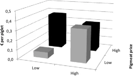
The results suggest that the value of sow space is responsive to changes in piglet and feed prices. In addition, the price of pigmeat also plays a role because changes in piglet price also depend on the price of pigmeat. Figure 3 represents farrowing farm’s loss due to choosing contract option 3
instead of option 1. Results suggest that a farrowing farm may loose in the long run when choosing contract option 3, where piglet price changes simultaneously with pigmeat price index. Hence, option 3) would be feasible if the farrowing farm is compensated for choosing this option. Moreover, the loss would be higher than low pigmeat price. The result is mainly due to expectations about prices. According to Table 1, the higher pigmeat price, the more likely it is to decrease in the near future. The outcome however depends on ratio at which the price changes are fixed. Figure 4 represents similar results for the case of high feed price.
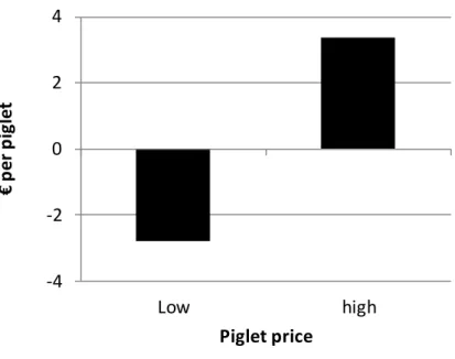
Results suggest that the farrowing farm has in most cases little incentives to sign the contract. Sensitivity analysis however shows that if all prices were random walk, then a farrowing farm would benefit from the contract in a favourable market situation (i.e. when output prices are high compared to input prices (see e.g. Figure 5). Higher overall impacts in Figure 5 than in 3 and 4 were because fixing the pattern of price change has a more persistent effect on relative prices in Figure 5.
Another sensitivity analysis suggests that extra costs reported in Figures 3 and 4 could typically be somewhat smaller if price volatility would be increased. Decrease in costs varied by scenario. High feed price scenarios and high pigmeat price scenarios showed a decrease in costs whereas having all three prices at the low level showed an increase in the costs.
In the data there was a correlation between piglet and feed prices. This implies that even if feed prices were soaring, and production costs of piglets, the price of piglets would be affected only gradually. By contrast, pigmeat price is more strongly correlated with feed price and thus changes in feed prices may be seen more rapidly in pigmeat price than piglet price. Historical data suggests that pigmeat price has been less volatile than piglet price. This observation is related to piglet price volatility in the early 2000’s. Hence, contract option 3 could also decrease the volatility of piglet
price. In a favourable (unfavourable) market situation the prices were expected not only to be less volatile but also to stay at a high (low) level for a longer time than in the event of option 1.
Low High 0,0 0,1 0,2 0,3 0,4 0,5 Low High P ig m e at pr ic e € pe r pi gl e t Piglet price
Figure 3. Reduction in the return on sow space (scaled to per sold piglet) under contract option 3 (changes in piglet price follow changes in pigmeat price) compared to option 1 (status quo) in the event of low feed price (November 2011 -20%; low and high pigmeat prices represent -/+18% from
November 2011, respectively). Low High 0,0 0,1 0,2 0,3 0,4 0,5 Low High P ig m e at pr ic e € p e r p ig le t Piglet price
Figure 4. Reduction in return on sow space (scaled to per sold piglet) under contract option 3 (changes in piglet price follow changes in pigmeat price) compared to option 1 (status quo) in the event of high feed price (November 2011 +20%; low and high pigmeat prices represent -/+18%
-4 -2 0 2 4 Low high € p er p ig le t Piglet price
Figure 5. Change in return on sow space (scaled to per sold piglet) under contract 3) at two alternative piglet prices (November 2011 +/-18%) in a sensitivity analysis scenario where pigmeat, feed and piglet prices follow random walk.
3.2. Finishing pigs
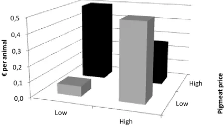
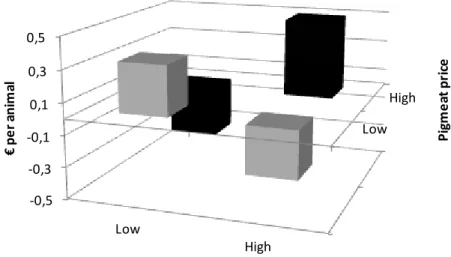
In the finishing pig particularly changes in pigmeat price have large impact on return on pig space unit. However, also feed and piglet prices are of importance. Figures 6 and 7 show how return on finishing pig space, when scaled down to per finished animal, is affected by the producer switching from contract type 1 to contract type 3. If feed price is initially low, finishing farm has economic incentives to sign the contract. By contrast, if feed price is high, the incentives depend on other market situation. The combination of low piglet and low pigmeat price or the combination of high piglet and high pigmeat price are in favour of the contract. In the latter case the result is related to the favourable market situation and in the former case it is related to expectations about more rapid piglet price increases in the future price. On the other hand, if price movements would be fixed in a
high pigmeat and low piglet price situation, then parameters in Table 2 could imply a more rapid expected decrease in piglet price than status quo
Increasing the price volatility through the distribution of weekly price changes in the finishing pig model increases both the return on pig space the volatility of return. Due to increased price volatility, decisions taken by the farm manager to maximize return also become more important. Figure 8 represents a sensitivity analysis scenario where the volatility of weekly price changes is increased by 40%. The results suggest that when price changes become more volatile, the contract becomes less attractive to the finishing farm. That holds particularly when pigmeat prices are low.
In the event that all prices follow random walk (Figure 9), the results are more straightforward than in comparable situations Figure 8. If pigmeat and piglet prices are high, the producer seems to benefit from the contract whereas if they are low, it is the opposite case. This result is related to the pattern how prices are linked to each others. As mentioned previously, pigmeat price is more strongly correlated with feed price that piglet price and changes in feed prices may show more rapidly in pigmeat than piglet price. Historical data suggests that pigmeat price has been less volatile than piglet price. If changes in piglet and pigmeat price are fixed to be similar when both prices are at a low level, then by definition, piglet prices can be high when also pigmeat prices are high. This could be unfavourable to a finishing farm in the sense that an increase in pigmeat price would result in a more rapid increase in piglet price as well. However, there is also another aspect, viz. that linking piglet and pigmeat prices more could increase the simultaneity of changes in production costs and receipts. This may affect finishing farm’s results.
The value of option to pause pig finishing operation temporarily in a poor market situation is included in results reported in Figures 6 and 7. However, when using parameter values in Table 2
the value of this option is typically small. The option to pause production becomes more valuable if the prices are random walk, and the value rises even more, if the correlation between price movements is broken down. Figure 9 shows the value of option to give up producing pigs temporarily as a function of current pigmeat price when all prices follow random walk. In the previously reported scenarios the role of option to pause pig finishing operation is quite small because the price of pigmeat is rather high compared to piglet price. However, if pigmeat prices were to decrease (ceteris paribus), then value of the option to have a production break could increase substantially. Low High 0,0 0,1 0,2 0,3 0,4 0,5 Low High P ig m e at pr ic e € pe r ani m al Piglet price
Figure 6. Change in return on finishing pig space (scaled to per finished animal) under contract option 3 (changes in piglet price follow changes in pigmeat price) compared to option 1 (status quo) in the event of low feed price (November 2011 20%; low and high pigmeat prices represent
Low High -0,5 -0,3 -0,1 0,1 0,3 0,5 Low High P ig m e at pr ic e € pe r ani m al Piglet price
Figure 7. Change in return on finishing pig space (scaled to per finished animal) under contract option 3 (changes in piglet price follow changes in pigmeat price) compared to option 1 (status quo) in the event of high feed price (November 2011 +20%; low and high pigmeat prices represent
-/+18% change from november 2011, respectively).
Low High -0,7 -0,5 -0,3 -0,1 0,1 0,3 0,5 Low High P ig m e at pr ic e € pe r ani m al Piglet price
Figure 8. Change in return on finishing pig space (scaled to per finished animal) under contract option 3 (changes in piglet price follow changes in pigmeat price) compared to option 1 (status quo) in the event of low feed price (November 2011 +20%; low and high pigmeat prices represent
-/+18% from change November 2011, respectively) when the volatility of price changes is increased by 40%.
-4 -2 0 2 4 Low High € p er p ig
Pigmeat and piglet price
Figure 9. Change in return on finishing pig space (scaled to per finished animal) under contract 3) at two alternative piglet prices (November 2011 +/-18%) in a sensitivity analysis scenario where pigmeat, feed and piglet prices are random walk and pigmeat and piglet prices are both either at high (November 2011 +18%) or low (-18%) level.
1,05 1,15 1,25 1,35 1,45 1,55 Ret u rn o n p ig s p ac e
Pigmeat price € per kg
Figure 10. The value (return on pig space per year) of option to temporarily pause pig fattening as a function of the price of pigmeat upon signing the contract when prices are random walk.
4. Discussion an conclusions
This paper has analysed how different contract options affect the value pig space unit in farrowing and finishing farm. Results provide valuable information on designing the contract coordination mechanisms in which also all producers are committed to maximize the value of the supply chain when the pigmeat market exhibit significant volatility. They provide insights to how input and output prices and their volatility affects return on pigs space unit in finishing and farrowing farms. Results suggest that if the option to suspend production temporarily is taken away by the flow scheduling contract, the value of pig space unit decreases as more return is obtained for the risk. The option to suspend production is the most valuable when market situation is unfavourable because then it can help the producer in avoiding large economic losses. The threshold price below which the option to suspend production is exercised, depends on how much variable costs can be saved by taking a pause in finishing pig production. In addition, the value of option is reduced by the fact that output prices tend to adjust to increases in input prices over time. Hence, in our results this option didn’t play a major role.
A key question in this paper is whether contract option 3 is feasible. When results from farrowing farm and finishing farm are taken together, it is noticed that contract option 3) is not always feasible. In cases where the contract is feasible it usually requires finishing farm to pay a fee to the farrowing farm. In the event of low feed price the contract is feasible in other cases except when both pigmeat and piglet price are high. By contrast, in the event of high feed price, the contract is feasible when either pigmeat of piglet price is low and the other price is high. Also when all prices follow random walk, there seems to be a price range where the contract is feasible.
Besides current market situation, the value of contract can also depend on price expectations. Price expectations can make the situation complex if covariates which imply that price changes depend on each others or from the market situation. During 2000 to 2011 pigmeat price in Finland was less volatile than piglet price, and there was quite small correlation between piglet and feed prices. This implies that even if feed prices are soaring, and thus increasing production costs of piglets, the price of piglets is likely to change only gradually. By contrast, pigmeat price is more strongly correlated with feed price and thus changes in feed costs may be transmitted more rapidly to pigmeat price than to piglet price. The results illustrate that the lack of appropriate contracts and inelasticity of piglet prices can result in distortions in the piglet market. The contract option preferred by producers depends on the relative prices and current status of the market. In general, results suggest that compensation that attracts finishing farms to sign the contract giving up this option is the higher the lower current pigmeat price is. Alternatively, farrowing farms could secure their piglet sales by allowing piglet price to follow changes in the price of pigmeat. In such a transparent contract finishing farms might not have an incentive to pause production. However, also farrowing farms may be reluctant to accept the contract if prices are unfavourable upon signing the contract. It can be expensive for an agent selling the piglets to have the finishing farm to fix the flow of production when pigmeat price is unfavourable, or to the farrowing farm to have piglet price fixed to pigmeat price if the market situation is not in favour of such a commitment. Therefore the commitments should be negotiated when the market situation is fairly good to both parties.
5. Acknowledgement
This paper is based on results from two separate research projects. Funding from the Ministry of Agriculture and Forestry for funding The Finnish Cultural Foundation, Finnish Animal Breeding
Association and the Central Union of Agricultural Producers and Forest Owners (MTK) is gratefully acknowledged.
6. References
Bellmann, R. 1957. Dynamic Programming. New Jersey: Princeton University Press. 339 p. Burt, O.R. 1965. Optimal replacement under risk, Journal of Farm Economics 47: 324-346. Burt, O.R. 1993. Decision rules for the dynamic animal feeding problem. American Journal of
Agricultural Economics. 75: 190-202.
Dubois, P. & Vukina, T. 2009. Optimal incentives under moral hazard and heterogeneous agents: evidence from production contracts data. International Journal of Industrial Organization 27 (4): 489-552.
Glen, J.J. 1983. A dynamic programming model for pig production. Journal of Operational Research Society vol. 34, 6, 511-519.
Hinrichs, J., Mußhoff, O. & Odening, M. 2008. Economic hysteresis in hog production Applied Economics 40 (3): 333 – 340.
Hayashi, F. 2000. Econometrics. New Jersey: Princeton University Press. 683 p.
Huirne, R.B.M., Dijkhuizen, A.A., van Beek, P. & Hendriks, Th.H.B. 1993. Stochastic dynamic programming to support sow replacement decisions. European Journal of Operational Research 67: 161-171.
Jalvingh, A.W., Dijkhuizen, A.A. & van Arendonk, J.A.M. 1992. Dynamic probabilistic modelling of reproduction and replacement management in sow herds. General aspects and model
Kristensen, A.R. & Søllested, T.A. 2004. A sow replacement model using Bayesian updating in a three-level hierarchic Markov process: II. Optimization model. Livestock Production Science 87: 25-36.
MTT, 2012. Results of Finnish Farm Accountancy Data. www.mtt.fi/economydoctor. Last visited 5 June 2012.
Niemi, J.K. 2006. Dynamic programming model for optimising feeding and slaughter decisions regarding fattening pigs. Agricultural and Food Science 15, Supplement 1: 1-121. Dissertation. https://oa.doria.fi/handle/10024/3334?locale=len
Niemi, J.K. & Lehtonen, H. 2010. Modelling pig sector dynamic adjustment to livestock epidemics with stochastic-duration trade disruptions. European Review of Agricultural Economics (in press). doi: 10.1093/erae/jbq047
Niemi, J.K., Sevón-Aimonen, M.-L., Pietola, K. & Stalder, K.J. 2009. The value of precision feeding technologies for grow–finish swine. Livestock Science 129: 13–23.
http://dx.doi.org/10.1016/j.livsci.2009.12.006
Odening, M. Mußhoff, O & Balmann, A. 2005. Investment decisions in hog finishing: an application of the real options approach. Agricultural Economics 32: 47–60.
OECD-FAO 2010. OECD-FAO agricultural outlook 2010-2019. OECD: Paris.
Pennings, J. & Wansink, A. (2004). Channel Contract Behavior: The Role of Risk Attitudes, Risk perceptions, and Channel Members’ Market Structures. Journal of Business 77: 697-723. Pietola, K.S. & Wang, H.H. 2004. The value of price- and quantity-fixing contracts for piglets in
Finland. European review of Agricultural Economics 27 (4): 431-447.
Plá, L.M. 2007. Review of mathematical models for sow herd management. Livestock Science 106: 107-119.
Trigeorgis, L. 1996. Real Options. MIT Press: Cambridge.
Richardson, J.W. & Condra, G.D. 1978. A general procedure for correlating events in simulation models. Department of Agricultural Economics, Texas A & M University, Mimeo, May 1978.
Richardson, J.W., Klose, S.L. & Gray, A.W. 2000. An applied procedure for extimating and simulating multivariate empirical (MVE) probability distributions in farm-level risk assessment and policy analysis. Journal of Agricultural and Applied Economics 23: 299-315.
Serenius, T., Sevón-Aimonen, M.-L., Kause, A., Mäntysaari, E. & Mäki-Tanila, A. 2004. Selection potential of different prolificacy traits in the Finnish Landrace and Large White populations. Acta agriculturae Scandinavica. Section A Animal science 54, 1: 36-43.
Statistics Finland. 2012. Statistical database. Index of purchase prices of the means of agricultural production and Index of producer prices of agricultural products.
http://www.tilastokeskus.fi/til/maa_en.html. Last visited 4 June 2012.
Uusitalo, P. & Pietola, K. 2002. Franchising-sopimukset sikatalouden hintariskien hallinnassa. Maa- ja elintarviketalous 11. Helsinki: MTT taloustutkimus. 35 p.
Uusitalo, P. & Pietola, K. 2001. Teknologiavalinnat ja sopimukset Suomen sikatiloilla. Helsinki: Maatalouden taloudellinen tutkimuslaitos. Tutkimuksia 249: 114 p.
Vukina, T., Shin, C. & Zheng, X. 2009. Complementarity among alternative procurement arrangements in the pork packing industry. Journal of Agricultural & Food Industrial Organization 7 (1): article 3.
Zheng, X, Vukina, T. & Shin, C. 2008. The role of farmers' risk aversion for contract choice in the US hog industry. Journal of Agricultural & Food Industrial Organization 6 (1): article 4.