Storage of Network Monitoring and Measurement Data

(1)

Storage of Network Monitoring

and Measurement Data

A report

submitted in partial fulfillment of the requirements for the degree

of

Bachelor of Computing and Mathematical Sciences

at

The University of Waikato

by

Nathan Overall

c

(2)

Abstract

Despite the limitations of current network monitoring tools, there has been little investigation into providing a viable alternative. Network operators need high resolution data over long time periods to make informed decisions about their networks. Current solutions discard data or do not provide the data in a practical format. This report addresses this problem and explores the development of a new solution to address these problems.

(3)

Acknowledgements

I would like to show my appreciation to the following persons who have made this project possible.

Members of the WAND Network group for their continued support during the project, including my supervisor Richard Nelson. I would also like to give a special mention to Shane Alcock and Brendon Jones for their ongoing assistance to the project while they developed the WAND Network Event Monitor.

DR. Scott Raynel for his support and advice throughout the project.

The WAND network group and Lightwire LTD for providing the resources necessary to conduct the project.

(4)

List of Acronyms

CLI Command Line Interface

RRD Round Robin Database

RRA Round Robin Archive

MRTG Multi Router Traffic Grapher

AMP Active Measurement Project

ISP Internet Service Provider

ICMP Internet Control Message Protocol

VoIP Voice over Internet Protocol

API Application Programming Interface

SNMP Simple Network Management Protocol

OpenTSDB Open Time Series Database

PDP Primary Data Point

CDP Consolidated Data Point

DS Data Source

RTT Round Trip Time

RAID Redundant Array of Independent Disks

SSD Solid State Drive

MB megabyte

GB gigabyte

TB terabyte

(7)

List of Figures

2.1 Layout of an RRD File . . . 5

3.1 Source: http://www.mkomo.com/cost-per-gigabyte . . . 13

3.2 Source: http://kaioa.com/node/74 . . . 13

3.3 Architecture within WAND Network Monitoring Project . . . 17

3.4 Diagram of Architecture . . . 18

3.5 Database Schema . . . 19

(8)

Chapter 1 Introduction

Network operators use monitoring software to help them operate and manage networks. There is no single system that provides all features they require. Instead they use a myriad of individual systems, which an administrator must navigate every time they want to view any data. If you have customers relying on your network then the time to resolve an issue is critical. To reduce the time consumed examining each location, data must be aggregated into a single location. This provides a central point of storage and retrieval of the data collected by the various tools available. During a network disruption network operators would then only need to look in a single location to see all the currently available data, ensuring they have the best information available to diagnose a problem.

1.1 Network Operation

Networks contain many diverse links, experience varying usage patterns, and include many, often different, devices. They also suffer from congestion, loss, latency, and an almost infinite list of other factors. Due to the myriad of different variables that can be in play, it is necessary to collect data about the operation of a network for a multitude of different situations. Efficient network operation requires knowing what areas of the network need improving and where problems are occurring. For this reason the collected data must be processed and analysed for anomalies. When these anomalies occur a network operator can be alerted to the problem, so they can deal with the issue as soon as it occurs. The data must also be stored to allow retrospective analysis of long term trends and historic events. This analysis will indicate how quickly

(9)

Chapter 1 Introduction 2

the resources are being consumed in a particular area and how long before upgrades are required or new equipment purchased.

1.2 Overview of the Problem

The problem is storing and managing the data effectively for network opera-tors. Investigation revealed that an existing solution that met all requirements did not appear to exist. Existing solutions often failed to be modern by not adapting to changes in hardware since they were invented. Others were difficult to set up, often requiring long set up procedures. Commonly used solutions were developed over a decade ago and suffer from limitations imposed due to the available hardware at the time. Due to these limitations the old solutions restrict the usefulness of the data and do not provide the data at the required resolution to run a modern network efficiently.

1.3 Goals

The goal is to provide an improved and modern storage system for Network Monitoring Data. The goals are built around the anticipated use within a network.

• Firstly the data resolution must be as high as is feasible on modern hardware

• Large amounts of data must be storable (e.g. five minute intervals for ten years) for a large number of different attributes measured.

• All attributes of a single monitoring feed must be tunable (how often and how long to store a copy of the data)

• The software must be scalable. Networks can involve a large number of nodes each providing a large number of data items.

• Flexible output provided for analysis of data

(10)

Chapter 1 Introduction 3

1.4 Plan of Action

The produce an effective final solution requires three main stages. Firstly the problems with the existing solutions must be identified in depth to expose the exact constraints the apply on the data. From these constraints investigation must be done to find the ideal solution that is feasible on modern hardware. Finally a solution must be produced ensuring the original outlined constraints are addressed.

Making major changes will be difficult when the design is implemented. For this reason the design must be thorough enough to ensure later changes are kept to a minimum. To achieve this the design will need to build on the research and address the constraints identified in a conclusive manner. During implementation the design should be refined to ensure as many goals can be incorporated as possible. The solution will then need to go through a refining process as well to ensure the solution operates in an optimal manner. This will involve testing the software in a real network and evaluating the suitability of the implementation.

The end result needs to be a solution that developers can integrate additional functionality into. This will allow tools to be modified to use the new solution. Network operators can then migrate from their current storage methods to the new solution.

(11)

Chapter 2 Background

This chapter explores existing network monitoring tools in regards to stor-age. The particular focus is the advantages and disadvantages of key design decisions that influence the storage of monitoring data.

2.1 Introduction

Network monitoring tools fall into two broad categories. Specialised tools designed to do a single task, and network management platforms that attempt to provide everything in a single location. Only specialised tools are covered here due to their prominent use in the networking monitoring area. Zabbix, a popular management platform has far less installs(The Debain Project, 2012c) than Smokeping(The Debain Project, 2012b) and cacti(The Debain Project, 2012a).

Specialised tools covered here include RRDs, a popular method of storing net-work monitoring data. Then the use of RRDs within two prominent monitoring tools will be discussed in depth. This is followed by a brief summary on two additional tools that use other storage methods. Finally the integration with a tool currently in development is explored.

2.2 Round Robin Database

Round Robin Databases (RRDs) were born from an earlier project called Multi Router Traffic Grapher (MRTG). In 1994 Tobias Oetiker needed a way to visualise traffic crossing a 64kbps link to the Internet. He created “a quick hack which created a constantly updated graph on the web”(Oetiker, 2012c).

(12)

Chapter 2 Background 5

During it’s life, speed became an issue for MRTG and large amounts of code were rewritten. In 1999 Oetiker announced RRDs as a solution for the speed issues people were suffering from with MRTG (Oetiker, 1996).

Since their incarnation there has been four additional major versions with all but the first still supported. The major focus with the updates has been on improving the graphs over changes to how the data actually managed(Oetiker, 2012b).

Figure 2.1: Layout of an RRD File

RRDs start with Data Sources (DSs). DSs are descriptions of the data fed into the RRDs. For example in the case of Smokeping the DSs are uptime, loss, median, and the Round Trip Time (RTT) for each of the 21 Internet Control Message Protocol (ICMP) packets. Data can be stored in five different types. Gauge is used for the number of something (e.g. number of users logged in). Counter is used when the value is constantly increasing, and therefore the increase is what needs to be stored (e.g. bytes of traffic that has passed through a router).

Derive stores the difference between each value. This is similar to counter except the value can increase and decrease, while a counter can only increase. Derive is often used to calculate the rate of change.

(13)

Absolute is used when the value is reset when it is read. This is used on data that increases quickly and is likely to overflow a counter

Compute is used for storing the result of a formula run on other data sources within the RRD.

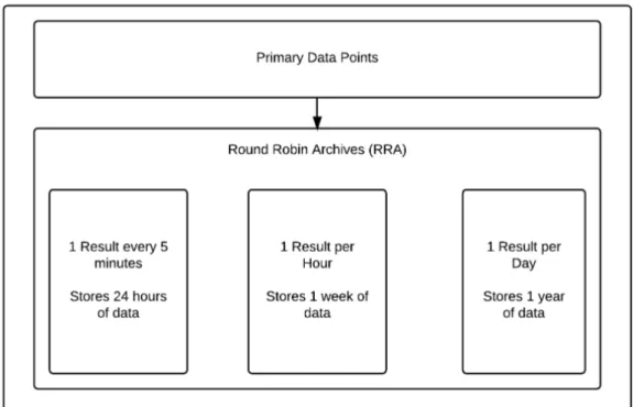
The actual values fetched and inserted into the RRDs are called Primary Data Points (PDPs) and are entered into the RRD at fixed intervals called steps (e.g. two minutes). PDPs that do not arrive on the step are interpolated. That is the previous and next PDPs are used to estimate what the real value would have been at the exact time of the step. The heartbeat value controls how late a PDP can be before it is inserted into the next step. A number of PDPs are then taken and stored inside a Round Robin Archive (RRA). A consolidation function is applied to a configured number of PDPs to convert them to Consolidated Data Points (CDPs) inside the RRAs. The consolidation function can be average(mean), minimum, maximum, or the last value. There are a number of RRAs within an RRD file which each specify a consolidation function and the number of PDPs per CDP. An RRA is essentially a database with a fixed number of rows. The RRA stores the index to the row it inserted CDPs into last, and uses the following row for the next set of CDPs. Through this process it continually overwrites the oldest values within the RRA. This is the round robin nature of RRD. Because the step, number of PDPs to each CDP, and number of rows in an RRA are fixed, each RRA represents a fixed amount of time.

RRA time period = interval * PDP per CDP * rows in RRA Function to calculate the time period covered by an RRA

So for example suppose an RRD has an interval of five minutes. It also contains an RRA that has 24 rows and consolidates 12 PDPs to each CDP. This means in total the RRA can hold 24 hours of data, with 1 point for every hour. Usually RRDs contain a number of RRAs with different attributes to cover different time periods. For example Smokeping by default uses uses a step of five minutes to update seven RRAs with three different time intervals. The three time periods are:

• 1 value every 5 minutes for 3 days 12 hours

(14)

• 1 value every 12 hours for 360 days.

There are a number of problems with this system. Firstly if a device on a network is performing poorly it can be beneficial to poll for data more regularly. The higher resolution data may be necessary to show the cause of the problem. However because RRDs force values to be within fixed intervals the RRD must be modified to support the new interval, This can be done using a tool called rrdtune. rrdtune will insert blank data and interpolate current values to work with the new interval. This leads to the second problem, reliability of data. Because RRDs interpolate some values, these values are not the real data, but an estimate of what the value likely was. In networking having the most accurate data possible is important to making decisions about the network. A network operator has no idea if they are looking at real or interpolated values. For example consider a sudden spike in traffic is recorded but because of the spike the value took 10 seconds longer to be inserted. The exact value recorded is likely to be lower if the network was operating normally before and after the spike in traffic. A network operator may then look at the data and decide the spike is not significant enough to warrant investigation, not knowing the values was actually much larger. Another problem with RRDs is the fixed size of the RRAs. This means eventually, depending on the attributes of the RRA, data will be overwritten. This was a sensible implementation when RRD were invented because disk space was limited. However disks have become much cheaper and substantially larger in size while the size of the data itself has stayed mostly static. This means we can record much more data today than we could 20 years ago when RRDs were implemented. However RRDs still only operate where the number of rows is specified at creation time, and therefore there is no way to add data indefinitely.

There are however benefits to the way RRDs operate. Firstly because the resolution of the data is slowly decreased, processing larger time periods does not take longer as there is a similar number of points in each RRA. Another benefit is that because a large number of tools use RRDs, if they were replaced a large number of tools could be utilized on the new system. This means there a major benefits to replacing RRDs in a way that the current tools can still work with.

Despite its flaws, RRD has became the de-facto standard for storage of network monitoring data. The RRD website lists in total 66 tools that use RRDs to

(15)

store data.(Oetiker, 2012a)

2.3 Tools using RRD

2.3.1 Smokeping

Smokeping is another creation by Tobias Oetiker (the inventor of Round Robin Databases) and uses RRDs to store its collected data.

Smokeping is a tool which periodically sends a number of ICMP echo packets to defined hosts and records the timing and number of the replies (also called pings). The main aim is to demonstrate places on the network where packets are either being dropped or lost (i.e. when the number of replies is less than the number of ICMP echos sent), and the amount of time between sending the ICMP echo and receiving the reply.

Smokeping demonstrates some of the limitations that RRDs have on network monitoring applications. There are a number of options configurable within Smokeping. One of these is how often the remote system is pinged. It may be useful to increase the regularity of pings to keep a higher resolution of data about a particular node of interest. However this will not be possible due to the fixed nature of RRDs. The opposite could also be the case. A node exists and then a decision is made to check the node less regularly. Again the only choice is to generate new RRD files. Two more useful configuration options are the number of ICMP echo packets sent and their size. It may be useful to send a greater number of packets to ensure a link is meeting stability expectations, while in other situations reducing the number of monitoring packets entering into the network could be useful. In relation to size, it is often good to check how a link performs on larger packets where large data transfers will take place. On the other hand a customer where Voice over Internet Protocol (VoIP) is a high percentage of their traffic is more likely to do many smaller packets and therefore the monitoring should reflect this.

There are several issue here that need addressing. One is to allow data to arrive any time and not specifically lock the data into timeslots. This will allow the adjusting of how often checks (in this case pings) are performed. The other problem outlined here is that of interpreting the data being recorded. To avoid this issue I’ll need to avoid making any distinction between different data types

(16)

being collected.

2.3.2 Cacti

Cacti is a popular graphing tool again based around RRDs. Cacti is a more general tool than Smokeping and can handle a wide variety different data types It was designed to “offer more ease of use than RRDtool and more flexibility than MRTG”(Goldman, 2007). Cacti comes with templates for a number of different devices which is a major reason for it’s popularity. Cacti uses a poller to fetch data either via Simple Network Management Protocol (SNMP) or by running scripts. The ability to run arbitrary scripts to collect data is widely used as SNMP can be difficult and time consuming to set up. The data is collected via a poller which is run at a regular interval to fetch the data. Cacti’s default poll time is five minutes although this can be reduced with some tweaking down to 1 minute. Bringing the polling below one minute is difficult because Cacti’s poller is triggered fromcron, a job scheduling daemon commonly used on Unix based operating systems. The minimum interval within cron is 1 minute, therefore running the poller more regularly would require use of a different tool to schedule to poller. Once again the use of RRDs causes a number of limitations. At the time of testing, Cacti does not tune the RRDs and therefore any changes made in cacti, for example to the polling time, will not be reflected in the RRDs. This could be problematic when it is necessary to reduce the polling time to a node for diagnosis reasons. Cacti also does not provide a good user interface for adding large number of new hosts. There is no easy to use command line interface that allows a script to add a number of hosts repeatedly. As it is common on a network to keep to a minimal number of different devices, the likeliness of adding the same device more than once is high. Cacti doesn’t do alerting based on thresholds, so another tool has to be used, which likely uses it’s own data sources (e.g. nagios), therefore the data is collected twice.

2.4 The Active Measurement Project

Active Measurement Project (AMP) is an application which runs scheduled tests against a list of nodes and reports back to a central location where the graphing software plots the results. AMP itself is divided into a series of components. The main component of AMP is the measurement software

(17)

that runs on each node. It conducts the tests at scheduled times. Next, the reporting software sends the results back to the central server. The central server stores and graphs the final data.

The WAND Group have been running AMP on a series of nodes distributed throughout New Zealand for many years now and have collected a large set of data. The nodes have been placed in locations of networking significance, such as Universities and Internet Service Providers (ISPs). The data collected will be useful for testing the final solution.

The problem with AMP is caused by how the data is stored. AMP stores all the collected data in flat text files. This made sense when it was initially developed as the expectation was that the most common data set accessed would be data relating to a given test on a given node. This required access and reading a single text file for data. Because data within a single file is usually allocated together, reading the data is generally fast. However if a request is made to look at data across all nodes for a given time period, the files of every node will need to be read. It is likely this data is scattered over a much larger area on the disk. This takes much longer to read and severely impacts on the performance. If the task being performed is generating a graph for a web page, then the data may never be retrieved before fetching the page is timed out by the web browser. The other issue is that if two users fetch the same data set they both end up waiting the same time period as there is no caching. I intend to solve both of these issues in my implementation.

To ensure these goals are achieved concurrent data access will need to be replicated and benchmarked to measure how the solution performs against the existing AMP system.

2.5 OpenTSDB

Open Time Series Database (OpenTSDB) is one tool that does not rely on RRDs. OpenTSDB does not delete or downsample data (The OpenTSDB Authors, 2012). The OpenTSDB was built for StumbleUpon to keep thousands of different Endpoints from thousands of Nodes. OpenTSDB is built upon HBase, a distributed and scalable data store. Due to its scalability it does have high minimum system requirements; the documentation implies you have a cluster of machines to run the software on. This potentially limits it’s

(18)

usefulness to large networks (in the order of thousands of Nodes). There is also a high knowledge requirement to work with the software. Most of the documentation is at a low level, (dealing with filesystems, compression, replication) which eliminates the option for easy and quick installation. HBase is an implementation of Google Big Table, which is used to store the data crawled off websites. Although this results in massive scalability for the project, it also adds a high level of complexity which is not needed in most networks and prevents it being deployed by many network teams.

2.6 WAND Network Event Monitor

WAND is currently working on a network monitoring project of its own. The idea of the project is to develop a system to detect when anomalies occur on a network and trigger alerts based on this data.

The work being conducted by the group requires a feed of data from multiple sources. As anomalies need to be detected as early as possible, writing the data to disk first and forcing the tool to read the written data wastes valuable time and resources. Instead the data needs to be passed directly into the anomaly detection system so alerts can be issued in real time. However the data would also need to be stored. This way when an alert is triggered the network operator can look at the relevant data and decide the best course of action. The needs of this project are particularly different to that of other tools which store the data, and read the stored data to produce the output (usually Graphs). In this case the data needs to be both stored as well as directly streamed into an additional tool.

2.7 Summary

To allow network operators to change from these existing tools a system for migration must be provided. Harvesting data from AMP and existing RRDs will be a necessary feature of the new solution.

Tight integration with the WAND Network Event Monitor will also provide a practical testing environment to work under. This will be helpful in ensuring the project is reliable and performs correctly while it is implemented.

(19)

Chapter 3 Design

3.1 Constraints

Before the design can be produced it is sensible to outline potential constraints which need to be addressed.

3.1.1 Hard Disks

Disks are the main permanent storage that Network Monitoring Data is gener-ally recorded to. Disks are relatively slow to access and the degree of slowness depends on a number of factors. These include proximity of data blocks, amount of data being read, speed of disk, and caching. When RRDs were invented disks were much smaller and therefore optimal use of disk space was critical. As discussed in section 2.2, RRDs preallocate the final file size during creation. This provided three benefits. Firstly the files would never grow and eventually exhaust disk space. Secondly an update would never fail to be saved because the disk was out of space. Lastly this avoids fragmentation which speeds up sequential data accesses.

As figure 3.1 shows, disks in 1994 cost round $1000 per Gigabyte. While in 2010 prices had fallen to just under $0.10 per GB, four orders of magnitude cheaper.

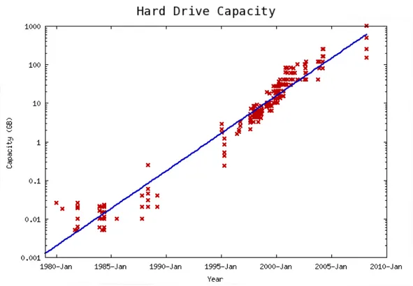
Not only have disks become cheaper but they have also grown in size substan-tially. Figure 3.2 shows that in 1994 disks were around 1 Gigabyte in size. By default Smokeping produces RRDs that are approx 3megabyte (MB) in size. Therefore on a 1gigabyte (GB) disk 341 RRD files could be stored. A network graphing 341 separate hosts is not unrealistic and demonstrates the need for

(20)

Chapter 3 Design 13

Figure 3.1: Source: http://www.mkomo.com/cost-per-gigabyte

Figure 3.2: Source: http://kaioa.com/node/74

caution when RRD was invented. In 2010 however it was possible to purchase 1TB disks, and today that has risen to around 3TB. Due to the reduced cost and increased size, it is possible for networks operators to maintain monitoring servers with several terabytes of storage available. In a single terabyte it is possible to store approximately 349,525 Smokeping RRD files. It is clear RRD

(21)

files have not adapted well to the continual increase in availability of disk space. It is also likely that disks will continue to increase in size and reduce in cost as both graphs indicate.

Disk performance has also increased continually since 1994 (Schmid, 2006). It is also common today for networks to operate a Redundant Array of Indepen-dent Disks (RAID) which combine a number of disks together for redundancy and more importantly speed. Reading from several disks at one time is sub-stantially faster over a single disk of equal size.

Another recent improvement in storage is Solid State Drives (SSDs). SSDs are several times faster at reading and writing than conventional hard drives. Although SSDs are not yet available in the substantial sizes available for conventional hard drives, it is worth noting their existence as something that may become prominent in the near future.

With all these changes, substantial improvements can be made over how RRD files operate.

3.1.2 Memory and Caching

Memory is much faster than disk but also far more scarce. Because memory is faster we want to utilize it to provide speed benefits were possible. However because it is limited, selecting the correct data to store in memory is an important decision that can’t be overlooked. The data use is the main driver here. If there is a website attached to the Network Monitoring Data displaying a series of graphs from certain Endpoint, then that data needs to be cached. On the other hand caching a task that processes large data sets which do not fit in memory is wasteful. A system for detecting when data should be cached would therefore be beneficial. Using memory efficiently can make a major difference to the responsiveness and therefore usefulness of a Network Monitoring Data storage system. Providing the ability to tune the level of caching will help network operators make the best utilization of memory when they need to improve performance.

Another possible way to speed up processing is to provide solutions for storing intermediate data during calculations. Then when the same calculation needs to be made on a slightly modified data set some values will not need to be recalculated.

(22)

3.2 Design Choices

The first problem to address is how to store the data. RRD chose a custom binary format to store data, while AMP chose text files. Both have major flaws which limited the usefulness of applications using the data. At this point it is important to consider tools that are specifically designed for dealing with data in a high performance manner. Databases are one such solution. Databases have been tuned to improve their performance over the last decade as the web has grown in size. Databases also have a number of interesting properties which would be beneficial to storing Network Monitoring Data. Databases try to allocate all of the data together, something AMP failed to do, while RRDs only achieved this by fixing the file size at creation time. This makes it much faster to read the data from the disk. Databases are also designed to operate well on systems such as RAID and SSDs. This allows them to operate efficiently despite the hardware they may be operating on. As use of RAID is common within networks and SSDs are becoming increasingly popular as fast alternatives to disks, it is of major significance that data can be read efficiently on these hardware configurations. As Databases are used in such a wide range of contexts from storing and retrieving web content, to archiving information for long term storage, they offer a very high level of flexibility. Unlike RRDs which had little development on the storage method after their invention, databases receive constant improvements. This means as improvements in software and hardware occur databases will take advantage of these to improve how they operate. Database have a number of methods to speed up accessing of data. One of these is indices. Indices are essentially a form of cache which speed up data retrieval by keeping an additional copy of data from the database. This data is stored in a way that can be accessed much faster. It can also be used to store data that is part of a calculation. For example suppose it is common to divide data recorded from a specific source by three, then this could be stored in the index. Therefore it is calculated when the index is created, and then as each value is inserted into the database. This is much faster than calculating values every time. There is however a trade off from these speed increases. Because an index is a copy of data already in the database, it takes up more disk space. However section 3.1.1 demonstrated how disk space is readily available, and getting cheaper over time, a trend which is likely to continue in the future. Databases also have internal systems to store commonly requested data in memory to avoid reading the same data

(23)

repeatedly. Efficient use of memory was something analysed in section 3.1.2. Databases also provide many ways to tune the use of memory. This may be useful if a network operator decides the speed of the database can be improved. As databases are core to many network operations, in large networks they are usually run on fast dedicated hardware. This also means network operators are familiar with maintaining databases and so a staff member would not need to gain new skills to operate software that uses databases. Choosing to use databases is therefore a sensible decision. However there are many types and flavours of databases. Initially it would be sensible to focus on databases commonly available within networks and possibly branch out to higher performance databases if time permits.

How to store data is the second major consideration. As discussed, RRDs overwrite old values due to their round robin design. Due to the increasing availability and reducing cost of disk space, it seems prudent to not impose any size limitations on stored data. Instead, if necessary, a pruning tool will be provided to reduce the consumed data by removing or aggregating selected data. Unlike the automatic and fixed basis RRDs does this on, it would be expected network operators will monitor the disk space usage and make the most appropriate decision for their network. They can then choose which data is less valuable and prune that appropriately meanwhile keeping more important data. This is unlike RRD which is usually configured with the same settings for every device regardless of it’s importance. Putting network operators in charge of their data is a major change to the current philosophy where the data is managed for them. However it is a wise move to improve the quality of the tools they have access to. These methods can always be automated by the network operators, but in a customized manner. Another feature of RRD was interpolating data. However as previously discussed modifying the values could degrade the quality of the data. Instead the data should be recorded exactly as it arrives. That is without interpolation of the data. However it may be still be useful to perform calculations on the data before it is inserted if it sensible to do so. For example with Smokeping only a handful of different statistics are actually shown on the graph, however the data is stored as its component parts. It would therefore make sense to calculate the values shown on the graph and store those in the database rather than storing extra unused data.

(24)

tools with something new, so it is important to provide a method of migration. In particular migrating existing data from RRDs and AMP will allow for their use within the new solution. Then an operator can choose to discontinue using the old storage systems when they are happy with the new solution.

As a major focus of the design is integration into the WAND Network Event Monitor it will be beneficial to design the solution within this context. Mean-while the improvements over other storage methods will be focussed on within this context. This will provide two benefits. Firstly this will ensure the design meets the needs of the project. Secondly it gives the design a real use context while it is designed. This will avoid many details that could possibly be overlooked if the solutions was designed as an isolated project.

3.3 Proposal

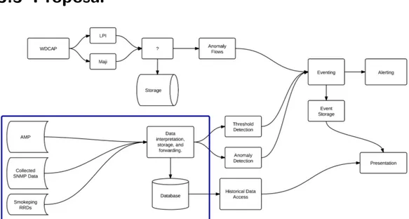
Figure 3.3:Architecture within WAND Network Monitoring Project

The box in Figure 3.3 demonstrates the components of the new solution within the WAND Network Event Monitor. Network Data is retrieved from existing RRDs in use by existing applications. This will provide a migration path from common existing tools such as Cacti and Smokeping. The whole point of this is to allow network operators to run the new solution alongside their current tools so they can feel comfortable not having to suddenly replace their current system and rely on something new. AMP can also be migrated. This will allow the AMP data to be imported and the speed issues that AMP suffers with focussed on.

(25)

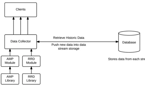
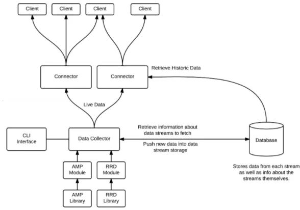
Figure 3.4: Diagram of Architecture

Figure 3.4 shows a break down of the internal structure. At the lowest level there are libraries for reading the various input types. These libraries should function in a standalone fashion and have no specific tie to the application. The next level is the modules. The modules are responsible for fetching the data using the libraries. Modules are stateful, that is they are not started purely for the purpose of obtaining data and then closed again. Instead it is the modules task to manage it’s resources and scheduling internally. This provides a few major benefits. Firstly this does not regiment the data collection in any way. The module can adjust it’s polling rate in real time if a value goes out of range for example. Modules could also be pushed based and listen on a socket for data from another program. This does however mean that modules must be thought out and resources used effectively. However it would be possible to create a module with minimal resources that merely calls a script on a regular interval if this was needed. Having modules start can store state and make decisions is a powerful tool an network operator can manipulate to produce the best data. Push based modules open interesting avenues. For example collecting data from device which are not always on, or connected to the network would be possible, without polling for its existence. This could be useful to collect data usage statistics from a mobile phone for example. The main application is called the data collector. The data collector instantiates and manages the modules as well as managing data transfer between the components. The data

(26)

collector receives data from the modules, stores it in the database, and finally forwards it on to listening clients. Internally a list of clients and what data streams they have subscribed to must be kept. Only sending the clients the data requested reduces the amount of data the clients have to deal with.

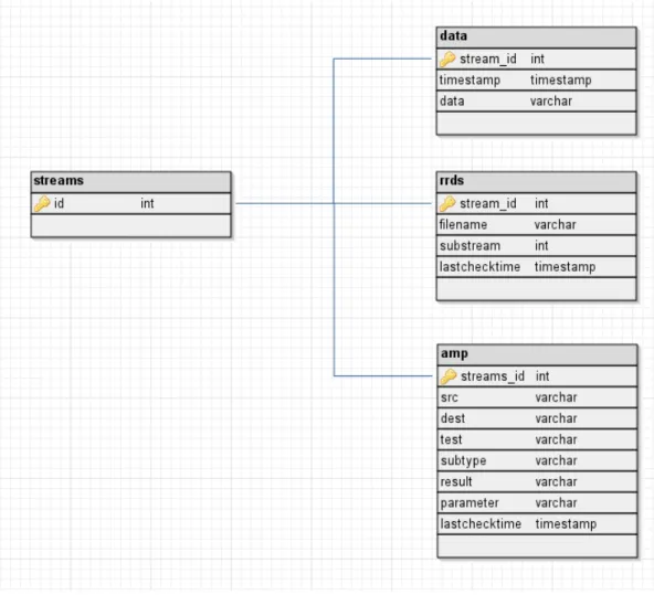
Figure 3.5: Database Schema

Due to the flexibility required, the input data format will be very simple. Firstly there is the streams table. This will only store the ids for the various streams. This will normally be joined to the individual module tables to find a particular module from by its id. Each module has its own table. This table is custom to each module and stores the any data the modules need during their operation. The most important table it the data table. This table has been kept very simple to avoid adding any limitations. There is the id of the stream the data came from, a timestamp when the data was recorded, and finally the data value. To store two different data values (e.g. input data and output data) two separate stream ids must be used. In general this is

(27)

not hugely efficient as to load any one data stream the other data must be parsed too. However as a general purpose storage this method works the best. Therefore all data will be stored in this way, and then separate partition tables will store copies any data that needs to be access faster. This avoid applying any restrictions around how the data is used. For example input data count and output data count from a network interface are almost always going to be read together. Therefore it is not sensible to generate a table for each of them when one table with both streams together would be more practical.

(28)

Chapter 4 Implementation

4.1 Resources

An early decision was to use the python programming language. Python has a low barrier to entry and offers rapid development. Choosing a language which is appropriate is important. Many network operators will have very limited coding skills but may still wish to make minor modifications to how the application operates. In particular is is likely they will want to customize the modules which may involve development depending on the completeness and customizability of the existing modules. In general Python produces manageable code. It achieves this by requiring white-space to indicate the control flow of the program. It also has a clean format that is generally easy to read. Rapid development is also a major benefit of Python. Python provides a large number of libraries and many more are available online, which avoids developers recreating code that already exists. It will also speed up the development time of the entire project which should free up some time to be focus on other issues within the project. For this reason libraries should be used unless code is not already available.

As libraries are beneficial to the productive use of time, a database abstraction library will be used. SQLAlchemy is by far the most mature library in this area. It has many advanced features that other libraries lack support for. For example, SQLAlchemy follows the pattern of not restricting the use of the database. It does not impose any special requirements beyond the limitations of the database itself. Some libraries force the tables and columns to be named in a particular way, while SQLAlchemy operates independent of naming conventions. SQLAlchemy also support a wide range of databases including

(29)

Chapter 4 Implementation 22

SQLite, Postgresql, MySQL, Oracle, MS-SQL, and several other less known databases. As the premise of the project is to be as flexible as possible though, SQLAlchemy still limits the types of databases that can be used. The database module will therefore be coded in an agnostic way, so that it would be swapped out for any alternate storage method with minimal amounts of additional development.

Postgresql is already set up on the machines available. This will therefore provide the testing database for development. If there is time available other databases will be set up and tested as well, however speed is likely to be similar between them, as they are differentiated more by feature set than speed.

4.2 Retrieving Existing Data

First the libraries to retrieve the data had to be coded. RRD files were worked on first due to their prevalence and availability. There is a general lack of documentation around the RRD format itself which caused a longer than expected period of investigation. Much of the RRD documentation assumed you were using the tools provided and therefore needed no understanding of the underlying system.

Two python libraries exist that interface with RRDs. rrdpython is the standard library developed by the authors of the original rrdtool. However rrdpython is coded in a very unusual way for python. C is code is often 3-5 times longer than the equivalent Python programvan Rossum (1997). The Python coding style reduces the time it takes to write code, as well as making it easier to edit later. In the end this library did not support the data retrieval required so it was discarded. The second library available is pyRRD. pyRRD is coded in a far more pythonic way and as such fits far more naturally into python code. Initial investigation showed the library was able to parse the data out of the RRDs. However it became apparently later this was not supported by the library. After initial failure with libraries it was necessary to implement a tool to read the RRDs. A command line tool is provided within the rrdtool package to export the contents of an RRD file. This was used to parse the data into the python library.

At the same time work was started on the AMP module as coding the libraries together would keep them more consistent. The AMP input module took

(30)

only a few hours work as the Application Programming Interface (API) is well written and returns data in a very easy to use fashion.

4.3 Modules

Modules need to be highly customizable while being easy to understand and modify. Modules consist of two components, the definition of the table within the database, and the data fetching. Both these components are clearly laid out within a module. This should be simple enough that most network operators will feel comfortable creating modules themselves.

The RRD and AMP modules use libraries to do the bulk of the heavy lifting. This helps abstract away any specific details to the implementations which provides relatively skeleton modules, good as examples that developers or network operators can copy and edit easily. They also store a last updated timestamp and show how to update this on the fly. The last updated times-tamp is necessary because AMP and RRD store data themselves. Therefore to collect only the data that has been added since the last check, the last updated timestamp is consulted, and only data after this point is added. This prevents duplicate data being added. It also demonstrates how a module can update a database value in its configuration table.

An important characteristic of modules is that they are run in a separate process to the data collector. Every module runs in its own process. This provides several benefits. In the past half a decade the number of processors within a computer has been rapidly increasing. A major benefit of multiple processes, is the ability to utilize these extra processors. It also cleanly sepa-rates separate tasks onto different processors, reducing the chances of the data collector slowing down due to limited processor time. If code in a module causes it to crash, only that thread will die, meanwhile the operation of the rest of the collector will continue. This model is critical in making the collector as resilient as possible.

4.4 Command Line Interface

A Command Line Interface (CLI) was implemented to manage the operations of the data collector at runtime. The problem here is implementing the

(31)

interface in a way that doesn’t disrupt the operation of the data collector. The CLI is therefore run in a separate thread. However there a slight problem with having the CLI in a separate process. As the data collector starts the process, these are referred to as child processes of the data collector and conversely the data collector is the parent of those processes. Only the parent of a thread can control and read information about it’s operation. As the CLI thread is started from the data collector it is also a child process of the data collector and therefore cannot control read information about of control how the other threads operate. As many of the operations from the command line will involve controlling the threads, such as starting and stopping the modules (which run in threads), a solution had to be implemented. It would be possible to make the CLI the parent process, but this would complicate the operation of the collector, something that needs to be avoided to ensure its reliability. Instead a messaging style system is used. When the CLI receives a command, it adds it to a list. Then when the data collector is not busy, it processed the commands in the list and swaps each command for its result. The CLI will pick up on this and return the data to the user. Although this can mean the operation within the CLI seems slow, it is unlikely to be a time dependant operation, and more often will be scripted or called from a web service.

4.5 Database

The initial schema had very few limitations and was flexible in almost any way. However a few problems resulted from this. The initial schema didn’t store the associated module name along with the stream id in the main stream table. Instead every module table was checked until the id was found. This meant the table for every module had to be checked to perform simple lookups for a streams module specific table. The inefficiency of this considerably reduced performance when many streams are running. Finding the balance between simplicity, flexibility, and speed is a tricky balance here. In this case extra data stored in the main table will reduce the lookup time by substantially. A field for the module specific table name was added to the streams table. This allows a quick check for the table name, and then another lookup in the required table. A field for a name was also added as it had been difficult up to this point to identify a specific stream. This forces every stream to have a name, even when it is one part of several streams that make up one piece

(32)

of data. However it is necessary for database maintenance, where old unused streams may want to be removed.

4.6 Forwarding Data

Initially a Unix socket was used to connect clients. The client would connect to the socket and send the ids of the data it was interested in. The collector would then add the client along with the ids it wanted to a list of clients to send data to. Every time data arrived the list would be consulted and if there was a match the data would be sent down the client’s socket. Sockets are not the most trivial sources to work with and raised the amount of knowledge required to use the tool. It also increased the complexity of the internal code and limited the output format to one type. Instead a simpler and more elegant solution needed to be developed. The entire client logic needed to be removed from the data collector and re-implemented in a new component named the ”connector”; as shown in figure 4.1.

Creating the connector as a standalone piece of software provided a number of benefits. Firstly the connector has no effect on the data collector in any way. As the data is the core of the whole application, and is intended to run constantly, anything that could disrupt its operation should be avoided. This is solved by the data collector sending all data to a multicast socket. A multicast socket operates by having a single sender and multiple listeners. The single input traffic is then shared to all the listeners. This sharing is done by the operating system itself locally or network hardware when passing over a network. The data is filtered internally within the connector and the relevant output passed on to the client. This separation also provides an easy way to manipulate the output system. Much like the input system, there will be a series of modules that provide various different output types. Be default Comma Separated Values is used, a very simple and easy to work with format. New output modules can be easily added much like the input modules. The connector is generally set up so there is one for every listener. This should not be an issue as there is almost no overhead due to the broadcasting of the data to each connector via the multicast socket. If this were unicast streams the data would need to be copied to each connector.

Modes of operation include fetching historical data and streaming live data. These can be used individually or together. The major drive behind this

(33)

configuration is efficient use of resources. Only those tools that are needed are enabled, saving on memory. This is useful if a large amount of historical data needs to be requested by a program in a way that doesn’t effect other processes on the same machine. If only had one connector this will likely cause issues for all clients. However in this situation the connector attached to this application can be run at a lower priority, while the others operate normally.

4.7 Architecture Modifications

It was discovered that large numbers of streams caused the program to slow down substantially. The problem was linked to an earlier decision of simplifi-cation. Instead of make a single module deal with all the streams of a given type the data collector started an instance of the module for every stream. This consumed substantial resources. Instead each module type is a separate instance. Each module is then responsible for every stream of that type. Although this reduces resources the modules are slightly more complicated. In this case the extra complexity is worthwhile to gain such a major speed improvement.

(34)

Chapter 5 Conclusion

5.1 Brief

The initial problem involved storing network monitoring data in an effective manner. The key to providing this involved investigating existing solutions to discover why they didn’t meet the needs of network operators. Several key problems were highlighted that needed to be solved. To provide data at the maximum resolution feasible on current hardware all data values are stored, regardless of when they arrive. Modern hardware was not a major limitation due to the dramatic increases in disk size. This also allowed for very large amounts of data to be stored. The input and output can be in any format providing the flexibility required for storage and retrieval of monitoring data in almost any application.

5.2 Progress

Currently the solution can read the best data from existing solutions and store that indefinitely. The two input modules provided read AMP and RRD data. It can also forward the data on to real time applications for analysis and alerting. Plugins provide CSV and socket output for historic and live data from the connector.

Testing was done against nodes that would be used in a real network, additional testing needs to be done to find the limits of the software, and in particular the database. Data aggregation is also not yet implemented. This is not critical as the main goal was to provided the best highest resolution data. At this point the solution can be deployed in real networks to begin collecting the data at a

(35)

Chapter 5 Conclusion 28

much higher resolution to their current solutions.

5.3 Future Work

Now that the base architecture is complete, developers can begin to add new plugins to the platform. This will be essential in migrating users away from RRD files. Current tools, such as cacti and Smokeping will need changes made for them to work from the new system. This will allow the new higher resolution data to be visualised.

Currently a database abstraction layer is provided which will work well in small to medium networks. In very large networks a more specialised data store may be necessary. This is definitely an area of future investigation. While the current provided solution is quick and easy to set up, large installations will likely want to push beyond the limits of standard databases. Testing the performance of column based databases will allow the solution to meet the demands of larger networks.

5.4 Contributions to the field

If the solutions is deployed in a widespread manner then it could cause a major change in network monitoring. The landscape of network monitoring has been dominated by RRDs for almost two decades now. This has limited the ability for network operators to record monitoring data in the detail they require to make informed decisions. Instead most have continued to use RRDs and allow their data to be interpolated and overwritten by newer data. Network operators have resisted changing due to the difficulty involved. However this solution provides an easy migration path which should give network operators time to gain confidence in it. When they are satisfied with the new solution they will be able to migrate over. It is also anticipated a community will build around the project providing a source of plugins for monitoring various network devices, appliances, and applications.

5.5 Summary

Many network monitoring tools today suffer from problems caused by storage tools. These problems limit the information available to network operators.

(36)

Chapter 5 Conclusion 29

With limited information network operators do not have the full picture of the network when making decisions. This project has developed a solution which provides migration from these existing restrictive storage systems. With this important improvement in monitoring data storage, network operators can make more informed decisions about their networks. This will improve the quality of networks, and therefore improve the overall user experience.

(37)

References

Goldman, G. (2007). Network management systems.

Retrieved fromhttp://isp-ceo.net/equipment/2007/cacti.html. Oetiker, T. (1996). ANNOUCNE: RRDtool 1.0.0.

Retrieved from https://lists.oetiker.ch/pipermail/rrd-announce/1999-July/ 000007.html.

Oetiker, T. (2012a). RRD World.

Retrieved fromhttp://oss.oetiker.ch/rrdtool/rrdworld/. Oetiker, T. (2012b). RRDtool Changelog.

Retrieved fromhttp://oss.oetiker.ch/rrdtool/pub/CHANGES. Oetiker, T. (2012c). What is MRTG ?

Retrieved fromhttp://oss.oetiker.ch/mrtg/doc/mrtg.en.html. van Rossum, G. (1997). Comparing python to other languages.

Retrieved fromhttp://www.python.org/doc/essays/comparisons.html. Schmid, P. (2006). Performance analysis.

Retrieved from http://www.tomshardware.com/reviews/ 15-years-of-hard-drive-history,1368-7.html.

The Debain Project (2012a). Popularity contest statistics for cacti. Retrieved fromhttp://qa.debian.org/popcon.php?package=cacti.

The Debain Project (2012b). Popularity contest statistics for smokeping. Retrieved fromhttp://qa.debian.org/popcon.php?package=smokepong. The Debain Project (2012c). Popularity contest statistics for zabbix.

Retrieved fromhttp://qa.debian.org/popcon.php?package=zabbix. The OpenTSDB Authors (2012). What’s opentsdb?

(38)

Glossary

cron Schedules jobs to run at regular intervals. The minimum interval is one minute . 9

Endpoint A single piece of information collected from a node . 10, 14

nagios A tool which runs checks on hosts and alerts if values exceed the

allowable range . 9

Network Monitoring Data Term used to refer to both network monitoring and

measurement data . 2, 12, 14, 15

Node A single piece of equipment that returns monitoring data . 10, 11

SNMP Protocol to manage devices on a network. Commonly used to fetch statistics about a device . 9

Storage of Network Monitoring and Measurement Data