Analyst
®
1.6.1 Software
Advanced User Guide
AB SCIEX
71 Four Valley Dr., Concord, Ontario, Canada. L4K 4V8. AB Sciex LP is ISO 9001 registered.
© 2012 AB SCIEX. Printed in Canada.
of this document or any part of this document is strictly prohibited, except as AB Sciex may authorize in writing.
Software that may be described in this document is furnished under a license agreement. It is against the law to copy, modify, or distribute the software on any medium, except as specifically allowed in the license agreement. Furthermore, the license agreement may prohibit the software from being disassembled, reverse engineered, or decompiled for any purpose.
Portions of this document may make reference to other manufacturers and/or their products, which may contain parts whose names are registered as trademarks and/or function as trademarks of their respective owners. Any such use is intended only to designate those manufacturers' products as supplied by AB Sciex for incorporation into its equipment and does not imply any right and/or license to use or permit others to use such manufacturers' and/or their product names as trademarks.
AB Sciex makes no warranties or representations as to the fitness of this equipment for any particular purpose and assumes no
responsibility or contingent liability, including indirect or consequential damages, for any use to which the purchaser may put the equipment described herein, or for any adverse circumstances arising therefrom.
For research use only. Not for use in diagnostic procedures.
The trademarks mentioned herein are the property of AB Sciex Pte. Ltd. or their respective owners.
Contents
Foreword. . . 7
Access System Documentation . . . .7
Contact Technical Support . . . .7
Chapter 1 General Information . . . 9
Analyst Service . . . .9
API Instrument Project Folders . . . .10
Program Files . . . .10
Projects and Subprojects . . . .11
Subprojects . . . .11
Project Organization . . . .12
Software Security . . . .13
Workspaces . . . .13
Chapter 2 Instrument Tuning and Calibration. . . 15
Automatic Tuning and Calibration . . . .15
Back up Instrument Parameters . . . .16
Restore Instrument Parameters . . . .16
Compound Optimization . . . .16
Flow Injection Analysis . . . .16
Infusion . . . .17
Chapter 3 Batches . . . 19
Batch Editor . . . .19
Batch Files . . . .20
Build a Batch as a Text File . . . .20
Import a Batch as a Text File . . . .20
Set Quantitation Details in the Batch Editor (Optional) . . . .21
Chapter 4 Device Methods . . . 23
Devices in Acquisition Methods . . . .23
Add or Remove an LC Device . . . .23
Set the LC Pump Properties . . . .24
Set the Autosampler Properties . . . .24
Set the Column Oven Properties . . . .24
Set the Switching Valve Properties . . . .25
Set the Diode Array Detector Parameters . . . .25
Set the Analog-to-Digital Converter Properties . . . .25
Dynamic Fill Time . . . .27
Experiments and Periods . . . .27
Experiments . . . .27
Periods . . . .27
Information Dependent Acquisition Methods . . . .28
Solvent Compressibility Values . . . .29
Spectra . . . .32
Background Subtraction . . . .32
Perform a Background Subtraction from a Spectrum . . . .32
Unlock the Ranges . . . .33
Background Subtract to File . . . .33
Perform a Background Subtraction to File . . . .33
Baseline Subtract . . . .34
Calculators . . . .35
Elemental Composition Calculator . . . .35
Hypermass Calculator . . . .35
Elemental Targeting Calculator . . . .35
Mass Property Calculator . . . .36
Isotopic Distribution Calculator . . . .36
Centroided Peaks . . . .36
Calculate the Centroid of a Peak . . . .36
Data Analysis . . . .37
Total Ion Chromatogram . . . .37
Extracted Ion Chromatogram . . . .37
Base Peak Chromatogram . . . .37
Extracted Wavelength Chromatogram . . . .38
Diode Array Detector . . . .38
Total Wavelength Chromatogram . . . .38
Overlay Graphs . . . .38
Cycle Between Overlaid Graphs . . . .39
Sum Overlays . . . .39
Graphs Labels . . . .39
Add Captions to a Graph . . . .39
Add Text to a Graph . . . .40
Compound Database . . . .40
Contour Plots . . . .40
View a Contour Plot . . . .41
Select an Area in a Contour Plot . . . .41
Set the Intensity and Absorbance in a Contour Plot . . . .42
Change Colors in a Contour Plot . . . .42
Dynamic Background Subtraction Algorithm . . . .42
Fragment Interpretation . . . .42
Connect the Fragment Interpretation Tool to a Spectrum . . . .43
Match Fragments with Peaks . . . .44
Select a Bond in a Molecular Structure . . . .44
View Isotopes . . . .44
Display a Formula Difference in a Spectrum . . . .44
Display a Formula Difference in the Fragment List . . . .45
Display a Formula Difference in a Molecular Structure . . . .45
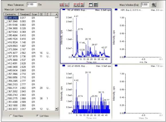
IDA Explorer . . . .45
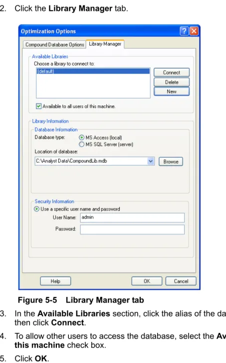
Library Databases . . . .46
Switch Between Existing Library Databases . . . .47
Connect to a Server Library Database . . . .48
View All Library Records . . . .49
Add a Record to the Library . . . .49
Search Library Records with Constraints . . . .50
Library Search Tips . . . .51
Search for a Similar Spectrum . . . .51
View a Compound from the Search Results . . . .53
Processed Data Files . . . .53
Save a Processed Data File . . . .53
Open a Processed Data File . . . .53
Qualitative Data . . . .53
Signal-to-Noise Ratio . . . .54
Smoothing Algorithms . . . .54
Smooth Data using the Smooth Algorithm . . . .55
Smooth Data using Gaussian Smoothing . . . .55
Spectral Arithmetic Wizard . . . .56
Toolbar Icons . . . .56
Chapter 6 Quantitative Data Analysis . . . 59
Calibration Options . . . .59
About Calibration Curves . . . .59
Select the Best Regression Type . . . .59
Integration Algorithms . . . .60
Analyst Classic and IntelliQuan Integration Algorithms . . . .61
Quantitation Method-Creation Tools . . . .62
Wizards . . . .62
Find Peaks Using an Automatic Method . . . .63
Quantitation Method Editor . . . .63
The Semi-Automatic Method Editor . . . .63
Find Peaks Using a Semi-Automatic Method . . . .64
Metric Plots . . . .64
Generate a Metric Temporary Plot . . . .65
Generate a Metric Plot and Save the Plot Criteria . . . .65
Save Default Plot Criteria for Future Results Tables . . . .67
Noise and Area Threshold Parameters . . . .67
Recalculate the Noise and Area Threshold . . . .68
Peak Integration . . . .68
Peak Review . . . .68
Peak Review Tips . . . .69
Detect Peaks . . . .69
Find the Potential Peak Start . . . .70
Confirm the Peak Start . . . .70
Find the Peak Top . . . .71
Find the Peak End . . . .73
Separate Peaks . . . .74
Queries . . . .75
Queries on Sample Type . . . .75
Default Queries and Table-Specific Queries . . . .75
Power . . . .78
Quadratic Calibration Equation . . . .78
Report Templates . . . .79
Customize Reports . . . .81
Preview, Print, and Export Reports . . . .81
Results Tables . . . .82
Define the Layout of Results Tables . . . .82
Sort Data in Results Tables . . . .83
Sort a Results Table and Save the Sort Criteria . . . .83
Save Default Sort Criteria for Future Results Tables . . . .84
Sort a Results Table using Preset Sort Criteria . . . .85
About using Queries with Results Tables . . . .85
Compare Results Between Batches . . . .85
How Concentration Levels Affect Results . . . .86
Results Table Layouts . . . .86
Summary Layout View . . . .87
Analyte Layout View . . . .87
Analyte Group Layout View . . . .88
Results Table Fields . . . .88
Results Table Tips . . . .94
Foreword
This Advanced User Guide provides information about the Analyst® software features.
Access System Documentation
The Help, guides, and tutorials for the instrument and the software are installed automatically. • Click Start > All Programs > AB SCIEX > Analyst. A complete list of the available
documentation can be found in the Help. • Press F1 to open the Help.
Contact Technical Support
The manufacturer and its representatives maintain a staff of fully-trained service and technical specialists located throughout the world. They can answer questions about the instrument or any technical issues that may arise. For more information, visit the Web site at www.absciex.com or contact Technical Support using [email protected].
1
General Information
The software is divided into discrete functional areas called modes. Modes allow the user to perform activities related to a main task. Modes are accessed through the Navigation bar or the Mode list in the toolbar. Users can switch from one mode to another without any loss of work. For more information, refer to the Analyst® software Show Me tutorial.
Analyst Service
The AnalystService is the communication path between the instrument and attached devices. The AnalystService is started each time the Analyst software is started. In general the Analyst Service starts automatically when the user logs on to Windows. If the service is not running when the Analyst software is started, then the Analyst Service will start automatically.
Figure 1-1 Analyst Software Window
Item Description 1 Mode list 2 Navigation bar
1
API Instrument Project Folders
The API Instrument project folder is important for the instrument to function properly. The API Instrument project contains the information required to tune and calibrate the system. The API Instrument project folder also contains data files for a manual tune that was performed using the Start button instead of the Acquire button. These data files are saved automatically in the API Instrument project folder in the Tuning Cache folder and named with the date and time they were created. Empty the Tuning Cache folder regularly.
The following are some of the folders found in the API Instrument project.
• API BioAnalyst: Contains the BTB Data Dictionary.csv file. This file contains the preset Data Dictionary information required for the BioAnalyst™ software. The appropriate folders appear only when the BioAnalyst software is installed. • Bundler: Contains a program that takes all aspects of a data file (.wiff file) and
automatically combines them when the sample is completed. • Configuration: Contains all the hardware profiles (.hwpf files).
• Example Scripts: Contains some of the scripts that are used with the software. • Instrument Data: Contains a file called InstrumentData.ins. The file stores all the
critical calibration information and more.
• Method Tables: Contains all instrument parameters that define the enhanced scan functions. Do not change the files in this folder. Changing the contents of this folder will affect the performance of the enhanced scan modes.
• Parameter Settings: Contains all the instrument parameters and linkages. Instrument parameters are saved as ParamSettingsdef.psf files.
• Preferences: Contains the Tunedata.tun file. All settings (parameter, tuning,
instrument, processing, appearances, and queue) are saved as Tunedata.tun in this folder.
• Processing Scripts: Contains the scripts for data processing in Explore mode. Scripts are found in the Script menu.
• Queue Data: Contains information from the queue.
• Tuning Cache: Contains all the data created in Manual Tuning by clicking Start instead of Acquire. Files are saved with a generic time and date stamp for their names. The Tuning Cache folder holds a limited number of files and will overwrite files as needed. Save the files with a new name and move the files immediately if they need to be saved.
Program Files
The following folders are found within the Program Files\Analyst folder.
• bin: Contains the software program files. Contents of this folder should not be changed as this will affect the software functionality.
• BioAnalyst Tutorial: Contains a tutorial that guides new users through all the features of the BioAnalyst™ software. A multimedia overview of the BioAnalyst software is also available. The folder is available only when the BioAnalyst software is installed.
General Information • Firmware: Contains the instrument system controller software (scu21.exe) and the
instrument firmware files. Use these files to download new firmware to the instrument when required. For more information, refer to the software installation guide included with the software.
• Help: Contains the help files, guides, tutorials, release notes and software installation guide.
• Scripts: Contains all the scripts that can be installed. Research-grade scripts are available to extend the functionality of the software. Some scripts are installed automatically and some scripts can be installed individually. For more information, refer to the Scripts User Guide.
• Simulation: Contains the instrument data files required to run the software in simulation mode.
Projects and Subprojects
Decide where to store the files related to the experiment before starting the experiment. Use projects and subprojects for each experiment to manage the data better and compare the results.
Subprojects
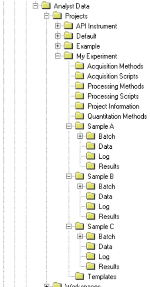
A subproject contains a subset of the folders in the project. All subprojects must contain the same folders. Subprojects are useful for organizing data.
For example, if samples of various compounds from different laboratories are run using the same acquisition method, then create subprojects to store the results for each laboratory, but leave the acquisition method folder in the project. The acquisition method is then available for use in the subproject or laboratory. Alternatively, if samples are being analyzed over a period of several weeks, then the results from each day can be stored in a separate subproject. Refer to Figure 1-2 Example of a project and subproject folder structure.
Figure 1-2 Example of a project and subproject folder structure
Project Organization
A project is a folder structure for organizing and storing sample information, data, quantitation information and so forth. Within each project there are folders that can contain different types of files; for example, the Data folder contains acquisition data files. Table 1-1 describes the contents of the different folders.
The software can access a project only if it is stored in a root folder. Users cannot create projects in a folder that has not been defined as a root folder.
The preset root folder is Analyst Data on the drive where the software is installed. To store projects in other locations, create new root folders. For more information about root folders, refer to the Help.
Table 1-1 Project Folders
Folder Contents
\Acquisition Methods Contains all acquisition methods used. Acquisition methods have the .dam extension.
\Acquisition Scripts Contains all the acquisition batch scripts available.
\Batch Contains all the acquisition batch files used. Acquisition batches have the .dab extension. It also contains a subfolder, Templates, that contains acquisition batch templates. Batch templates have the .dat extension.
General Information
Software Security
The software has a number of functions for configuring and managing security. The Analyst® software administrator can:
• Choose a security mode to best suit the needs of the operating environment. • Add and delete users and roles.
• Set access rights to users and roles as required. • Control access to remote instrument stations. • Control access to project files.
For more information about Analyst software security, refer to the Laboratory Director’s Guide.
Workspaces
A workspace is a particular arrangement of windows and panes, including any associated file or files. For example, while working on a particular data set, users can open and size various windows to help with the analysis. This arrangement, or workspace, can be saved so that the next time users look at the data, the window arrangement is identical.
In Quantitate and Explore modes, users can have multiple workspaces per session. This means that different workspaces can be designed to suit different tasks within these modes, and then save them for future use. When in one of these two modes, a particular workspace can be opened without exiting that mode.
\BioAnalyst Contains files used with the BioAnalyst™ software add-on, a protein analysis tool. The folder is available only when the BioAnalyst software is installed.
\Data Contains the acquisition data files (.wiff extension).
\Log Contains results of quantitation and compound optimization. \Processing Methods Contains all qualitative data processing methods used.
\Processing Scripts Contains all data processing scripts available. Processing scripts stored in the API Instrument project appear in the Scripts menu.
\Project Information Contains all project information and settings for the project. This folder cannot be stored in a subproject.
\Quantitation Methods Contains all quantitation methods used. Quantitation methods have a .qmf extension.
\Results Contains all quantitation results table files (.rdb extension). \Templates Contains report templates (.rpt extension).
Table 1-1 Project Folders (Continued)
2
Instrument Tuning and Calibration
Tuning the instrument is the process of optimizing the resolution and instrument parameters to attain the best sensitivity and performance of the system. Optimizing the resolution means adjusting the peak width and peak shape. Users can tune and calibrate the instrument either automatically or manually.
Automatic tuning: The software performs resolution optimization and mass calibration, using the Instrument Optimization wizard. For linear ion trap (LIT) instruments, MS3 optimizations are also performed.
Manual tuning: Users can perform many of the instrument resolution optimizations and calibrations manually.
Automatic Tuning and Calibration
Instrument Optimization is automatic instrument tuning software that tunes both quadrupole and LIT modes and performs mass calibration. For quadrupole mode, it adjusts the resolution offsets. For LIT mode, it optimizes AF3 and EXB. For MS3, it adjusts the excitation and isolation
coefficients. Select one of the instrument performance options:
• Verify instrument performance: Tests the instrument performance but leaves the instrument settings unchanged. A report is generated at the end of the test. Use this option weekly to check how well the instrument is performing.
• Adjust mass calibration only: Automatically checks and adjusts the mass calibration. If the mass calibration has changed, then the software corrects it. Use this option weekly for LIT instruments, or monthly to check and adjust the mass calibration if required.
• Adjust instrument settings: Checks and adjusts the instrument settings and mass calibration. The instrument settings are updated from the current settings to optimal settings. Use this option if instrument performance is poor or if the peak shape is bad. Only experienced users should adjust the instrument settings.
• Reset selected scan modes to default values and adjust instrument settings: Resets the instrument values to the factory preset values. Select this option if a major component of the instrument is replaced or after the first installation. Only FSEs should use this feature.
Back up Instrument Parameters
Back up the current instrument parameters in case they must be restored later. The preset location for the instrument parameters is C:\Analyst Data\Projects\API Instrument\Instrument Optimization\Instrument Settings Backups\User Created Backups.
1. In the Navigation Bar, double-click Instrument Optimization. 2. Click File > Backup Instrument Settings.
3. Type a file name. 4. Click Save.
Restore Instrument Parameters
1. In the Navigation Bar, double-click Instrument Optimization. 2. Click File > Restore Instrument Settings.
3. Navigate to the instrument settings. 4. Click Open.
Compound Optimization
The Compound Optimization software wizard automatically optimizes an analyte. Samples can be introduced using infusion or FIA (flow injection analysis.) The software first checks for the presence of the compounds. The voltages of the various ion path parameters are gradually increased or decreased to determine the maximum signal intensity (Q1 scan) for each ion. A text file is generated and then displayed during the optimization process. This file records the various experiments performed and the optimal values for each ion optic parameter. A file folder
containing all the experiments performed is also generated and can be found by opening the data file folder in Explore mode. For each experiment performed, an acquisition method is also generated and saved in the acquisition method folder.
Flow Injection Analysis
Flow Injection Analysis (FIA) is the injection of a small quantity of a sample by an autosampler into the LC stream. During the FIA optimization process, multiple sample injections are
performed for various source- or compound-dependent, or both, parameter types that are changed between injections. FIA optimizes for declustering potential, collision energy, and collision cell exit potential by performing looped experiments in succession, that is, one compound-dependent parameter followed by then next compound-dependent parameter. It optimizes for source-dependant parameters by making an injection for each parameter.
Use FIA optimization to optimize both compound- and source-dependent parameters using LC at higher flow rates.
Instrument Tuning and Calibration
Infusion
Infusion is the continuous flow of the sample at low flow rates into the ion source using a syringe pump. During the infusion optimization process, the software can select precursor and product ions and optimize for declustering potential, collision energy, and collision cell exit potential for both. The voltages of these ion path parameters are gradually increased or decreased to determine the maximum signal intensity for the precursor and product ions.
Use infusion optimization to optimize compound-dependent parameters only at much lower flow rates than those used during LC/MS analysis.
3
Batches
A batch is a collection of information about the samples to be analyzed. Samples are usually grouped into sets to make it easier to submit them. Grouping the samples into a set also reduces the amount of data that must be typed manually. A set can consist of a single sample or multiple samples. All of the sets in a batch use the same hardware profile, however, samples in a set can have different acquisition methods. A batch can be submitted only from an acquisition station. Batches link together:
• Sample information, such as name, ID, and comment. • Autosampler location (rack information).
• Acquisition methods.
• Processing method or script (optional). • Quantitation information (optional). • Custom sample data (optional). • Set information.
Batch Editor
Use the Batch Editor to create or modify batches and to create batch templates. To run samples, each using different acquisition methods, select multiple acquisition methods in the same set. An acquisition method can also be used as a template. In this case, the same method is used for each sample, but the user can select different masses or mass ranges for each sample. The Batch Editor can also be used to import sample lists created in external programs, such as Microsoft Excel.
The user can modify every detail of the batch before submitting it for processing. When a batch is submitted for analysis, the user can submit the entire batch, specific sets within the batch, or specific samples within a set.
For example, to analyze ten samples, five using one acquisition method and five using a different acquisition method, create a batch of two sets, one for each method used.
Table 3-1 Batch Editor Tabs
Tab Description
Sample Used to create the sample list and to select sample details such as the sample name and the acquisition method to be used to acquire the sample.
Locations Used to select the positions of samples in the autosampler. Sample locations can be specified numerically in the Sample tab, however, the Locations tab provides a graphical interface for selecting sample locations.
Quantitation Used to select the sample types and concentrations for quantitation batches. Because quantitation information can be specified post-acquisition in the quantitation Results Table, users do not have to use the Quantitation tab in the Batch Editor. Instead, the Quantitation Wizard can be used.
Batch Files
To make data entry easier, batch file information from other applications can be imported. The Batch Editor can import text and other files that are formatted correctly. For examples of correctly formatted files, refer to the Batch folder in the Example project.
The information in a batch file can also be exported for use with other applications, such as Microsoft Excel, Microsoft Access, and certain LIMS (Laboratory Information Management System) software.
Build a Batch as a Text File
Users can export a batch only if it contains at least one set with at least one sample. If the text file is saved, it can be used again later as a template.
1. Make sure that the active hardware profile includes all the devices needed to acquire the samples.
2. In the Navigation Bar, under Acquire, double-click Build Acquisition Batch.
3. Create a single-set, single-sample batch. 4. Click File > Export.
5. Name the file. 6. Click Save.
7. Open the text file in a spreadsheet program.
8. Type, or copy and paste, the details for the samples: one sample per row, with the details under the appropriate headings.
9. Save the modified text file as a .txt or .csv file. 10. Close the spreadsheet program.
The text file can now be imported into the Batch Editor.
Import a Batch as a Text File
Before batch information is imported from a text file, make sure the data in the file is organized and formatted correctly. In particular, the column headings in the spreadsheet must match the Batch Editor column headings.
1. In the Navigation Bar, under Acquire, double-click Build Acquisition Batch. Submit Used to verify sample information and to submit samples to the acquisition
queue. The Queue Manager shows queue, batch, and sample status and allows users to manage samples in the queue.
Note: Do not delete any of the columns. The columns in the spreadsheet must match the columns in the Batch Editor.
Table 3-1 Batch Editor Tabs (Continued)
Batches 2. In the Sample tab, right-click and then click Import From > File.
3. Click the text file containing the batch information.
4. Click Open.
If an autosampler is being used, then the Select Autosampler dialog opens. 5. In the autosampler list, select the autosampler.
6. Click OK.
The sample table fills with the details from the text file.
Set Quantitation Details in the Batch Editor (Optional)
If users do not want select quantitation details post-acquisition, then Quantitation methods can be included with a batch and used to define the quantitation details prior to submitting a batch. Internal Standard and Standard columns appear in the Quantitation tab according to the quantitation method selected in the Sample tab.
1. With a batch file open in the Batch Editor window, click the Quantitation tab. 2. Select the set.
3. In the cell, select a Quant Type for all the samples.
4. If applicable, type the peak concentration in the Analyte column. 5. If applicable, type the Internal Standard.
6. Repeat the preceding steps for each set in the batch. 7. Save the file.
Note: If the saved text file is not visible, then in the Files of type list, select Microsoft Text Driver (*.txt; *.csv). Files with the extension .txt appear in the field.
4
Device Methods
If creating an acquisition method file from an existing file, the user can use some or all of the device methods in the acquisition method. Use the Acquisition Method Editor to customize the acquisition method by adding or removing device methods. If the required device icon is not in the Acquisition Method Browser pane, then users can add the device only if it is included in the active hardware profile.
Devices in Acquisition Methods
Create an acquisition method for a device by selecting the operating parameters for that device. Acquisition methods can be created for any of the following devices if they are configured in the active hardware profile:
• Pumps. • Autosamplers. • Syringe pumps. • Column ovens. • Switching valves. • Diode array detector.
• Analog-to-digital converters. • Integrated systems.
For information about setting properties for devices, refer to the Peripheral Devices Setup Guide.
Add or Remove an LC Device
1. With a method file open in the Acquisition Method Editor, in the Acquisition method
pane, right-click Acquisition Method and then click Add/Remove Device Method.
Note: The available parameters for the LC devices vary depending on the manufacturer.
Figure 4-1 Add/Remove Device Method dialog
2. Select or clear the check boxes beside the device method to add or remove the device method.
3. Click OK.
Set the LC Pump Properties
1. With an acquisition method file open in the Acquisition Method Editor, in the
Acquisition method pane, click the Pump icon.
The Pump Properties tab opens in the Acquisition Method Editor pane. 2. Edit the fields as required.
3. Save the file.
Set the Autosampler Properties
1. Make sure that on the Acquisition Properties tab, the Synchronization Mode field is set to LC Sync. The device and the instrument will start simultaneously.
2. With a method file open in the Acquisition Method Editor, in the Acquisition method
pane, click the Autosampler icon.
The Autosampler Properties tab opens in the Acquisition Method Editor pane. 3. Edit the fields as required.
4. Save the file.
Set the Column Oven Properties
1. With a method file open in the Acquisition Method Editor, in the Acquisition method
pane, click the Column Oven icon.
The Column Oven properties tab opens in the Acquisition Method Editor pane. 2. Edit the fields as required.
Device Methods 3. Save the file.
Set the Switching Valve Properties
The switching valve can be used as a diverter or injection valve. Select the Manual Sync with Valve synchronization mode if using the valve as an injector; choose any other mode if using the valve as a diverter.
1. With a method file open in the Acquisition Method Editor, in the Acquisition method
pane, click the Valve icon.
The Valve Properties tab opens in the Acquisition Method Editor pane. 2. Change the position names from their preset names, if required.
The switching valve is sometimes used to switch the flow of solvent to waste, or to a different column. The preset position names are A and B.
• In the Change Position Names list, select a position.
• In the Change Position Names list, rename the preset position names A and B to Inject and Divert or to Column and Waste, depending on how the valve is plumbed.
3. In the Total Time (min) column, click a cell, and then type the total time the valve will remain in this position.
4. In the Position column, click a cell and then, in the Position list, select the valve position.
5. Repeat the steps 3 and 4 for each switch of the valve required during acquisition. 6. Save the file.
Set the Diode Array Detector Parameters
1. With a method file open in the Acquisition Method Editor, in the Acquisition method
pane, click the Diode Array Detector (DAD) icon.
The DAD Method Editor tab opens in the Acquisition Method Editor pane. 2. Set the desired acquisition parameters and save the file.
Set the Analog-to-Digital Converter Properties
1. With a method file open in the Acquisition Method Editor, in the Acquisition method
pane, click the Analog to Digital Converter (ADC) icon.
The Analog/Digital Convertor Properties tab opens in the Acquisition Method Editor pane.
2. In the Sample section, in the Rate (pts/sec) field, type the rate.
3. Do the following to set the channel details:
Note: The interval and rate are proportional to each other. When the rate is changed, the software automatically calculates the interval again.
• In the Channels field, click the channel name, and then select the check box beside the name to include it in the method.
• In the Interpreted Value @ Full Scale field, type the appropriate value. • In the Interpreted Unit field, type the appropriate unit.
The number of available channels is specified when setting up the ADC in the hardware profile.
Device Methods
Dynamic Fill Time
Dynamic Fill Time (DFT) is a feature specifically designed to optimize the data obtained in every spectrum for the linear ion trap scan functions. DFT will automatically adjust the fill time used to fill the ion trap based on the ion flux coming from the source. For more intense ions, the fill time will be automatically reduced to ensure the trap is not overfilled with ions.
For less intense ions, the fill time will be automatically increased, ensuring that good ion statistics are obtained in the spectrum. DFT is applicable for the following scan types:
• Enhanced MS (EMS) • Enhanced Resolution (ER)
• Enhanced Product Ion Scan (EPI) • MS/MS/MS (MS3)
Adjust the DFT settings by selecting Tools > Settings > Method Options in the software.
Experiments and Periods
The mass spectrometer acquisition method consists of experiments and periods. In the
Acquisition Method Browser pane, create a sequence of acquisition periods and experiments for the instrument. Users can also open a method previously created in the Tune Method Editor.
Experiments
An experiment includes the instrument settings and the scan type during an MS scan. A set of MS scans performed for a specific amount of time is called a period. An acquisition method in which the MS parameters and actions are the same through the entire duration is called a single-period, single-experiment method.
In looped experiments, MS settings are changed on a scan-by-scan basis. For example, if the sample contains two compounds, A and B, users may want to loop an MS/MS experiment of compound A with an MS/MS experiment of compound B to obtain information about both
compounds in the same run. The mass spectrometer method will alternate between the two scan types. Other examples of looped experiments include alternating between positive and negative modes in a run and Information Dependent Acquisition (IDA) methods.
Periods
A period can contain one or more looped experiments. In a multi-period acquisition method, experiments are performed for a specified amount of time and then switch to another set of experiments. Periods are useful when the elution time of the compounds in an LC run is known. The instrument can perform different experiments according to when the compounds elute to obtain as much information as possible in the same run.
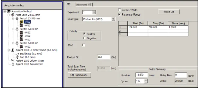
Figure 4-2 shows a three-period method. The first period has a duration of 3.015 minutes; the second period is 4.986 minutes; and the third period is 7.000 minutes.
Figure 4-2 Example of a multi-period experiment
Information Dependent Acquisition Methods
Information Dependent Acquisition (IDA) is an acquisition method that analyzes data during acquisition. IDA is used to change the experimental conditions depending on the analysis results. These real-time changes are controlled by criteria set in the acquisition method, including:
• Ion intensity and charge state. • Inclusion and exclusion lists. • Isotope pattern.
Optimizing data acquisition settings while the data is being acquired allows users to conserve both the sample and working time on an instrument.
Create an IDA method with up to two survey scans and eight dependent scans in a single experiment. A survey scan is used in IDA to trigger additional experiments. The following scan types can be used as a survey scan:
• Enhanced Multiply-Charged (EMC).
• Enhanced Product Ion (EPI) (second survey scan). • Enhanced MS (EMS).
• MRM.
• Neutral Loss (NL). • Precursor Ion (Prec). • Q3 MS.
The following scan types can be used as dependent scans: • EPI.
Device Methods In an IDA experiment, the instrument actions are varied from scan type to scan type based on the data acquired in a previous scan. The software analyzes data as it is being acquired and then determines the masses on which to perform dependent scans. Uses can set the criteria that will activate an IDA experiment and the method parameters to be used.
IDA experiments modify experiments and improve results based on the following user-defined criteria:
• Ion intensity and charge state. • Inclusion and exclusion lists. • Isotope pattern.
• Dynamic exclusion.
• Rate of change in ion intensity (refer to Contour Plots on page 40).
Solvent Compressibility Values
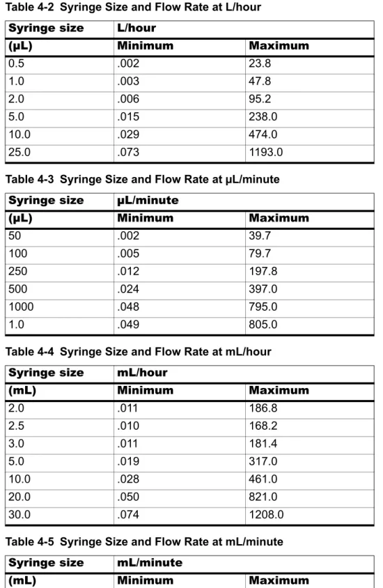
Syringe Size Versus Flow Rate
The flow rate of a syringe pump depends on the syringe installed in the pump. The following tables show the relationship between flow rate and syringe size.
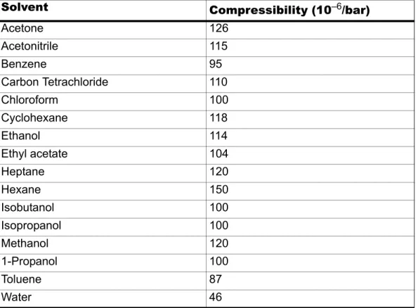
Table 4-1 Solvent Compressibility Values
Solvent Compressibility (10–6/bar)
Acetone 126 Acetonitrile 115 Benzene 95 Carbon Tetrachloride 110 Chloroform 100 Cyclohexane 118 Ethanol 114 Ethyl acetate 104 Heptane 120 Hexane 150 Isobutanol 100 Isopropanol 100 Methanol 120 1-Propanol 100 Toluene 87 Water 46
Table 4-2 Syringe Size and Flow Rate at L/hour
Syringe size L/hour
(µL) Minimum Maximum 0.5 .002 23.8 1.0 .003 47.8 2.0 .006 95.2 5.0 .015 238.0 10.0 .029 474.0 25.0 .073 1193.0
Table 4-3 Syringe Size and Flow Rate at µL/minute
Syringe size µL/minute
(µL) Minimum Maximum 50 .002 39.7 100 .005 79.7 250 .012 197.8 500 .024 397.0 1000 .048 795.0 1.0 .049 805.0
Table 4-4 Syringe Size and Flow Rate at mL/hour
Syringe size mL/hour
(mL) Minimum Maximum 2.0 .011 186.8 2.5 .010 168.2 3.0 .011 181.4 5.0 .019 317.0 10.0 .028 461.0 20.0 .050 821.0 30.0 .074 1208.0
Table 4-5 Syringe Size and Flow Rate at mL/minute
Syringe size mL/minute
(mL) Minimum Maximum
50.0 .002 28.40
100.0 .003 47.60
5
Qualitative Data Analysis
Users can view the information contained in a data file in table or graph form. Graphical data is presented either as a chromatogram or as a spectrum. Data from either of these displays can be viewed as a table of data points and various sorting operations can be performed on the data. The software stores data in files with a .wiff extension. Wiff files can contain data for more than one sample. In addition to .wiff files, the software can open .txt files; .txt files contain data for only one sample. When a data file is opened in the software, different panes appear depending on the type of experiment that was performed.
If the MCA check box is selected in the Tune Method Editor, the data file will open to the MS (mass spectrum). If the MCA check box is not selected, then the data file opens with the Total Ion Chromatogram (TIC). Users can select a range and then double-click in the TIC pane at a particular time to show the MS for this range.
Chromatograms
A chromatogram displays the variation of some quantity with respect to time in a repetitive experiment; for example, when the instrument is programmed to repeat a given set of mass spectral scans several times. Chromatographic data is contiguous, even if the intensity of the data is zero. Chromatograms are not generated directly by the instrument, but are generated from mass spectra.
In the chromatogram display, the intensity, in counts per second (cps), is shown on the y-axis versus time on the x-axis. Peaks are automatically labeled.
In the case of LC/MS, the chromatogram is often displayed as a function of time, the time at which a particular scan was obtained, which can be derived from the scan number.
When data is viewed as a spectrum, mass-specific information about a compound is obtained. A chromatogram provides a general view of the data, usually time dependent when using an LC column, but it does provide information about the components of a peak. A spectrum, however, looks at a particular peak and provides the molecular weight of the corresponding compound, which can be used to find more specific information. For example, while a chromatogram may show only one peak, that peak can represent more than one compound; that is, different masses. A spectrum shows all of the masses that make up a peak, including the intensity of each mass. Chromatographic data can change in both time and intensity if there is a change in the
chromatographic conditions in a given sample. Spectral intensities may change, but the masses are fixed because the mass of a compound does not change.
There are two ways to generate spectral data:
• If only one scan is acquired, then the data is shown as a spectrum. • From a chromatogram.
A typical spectrum is shown with the molecular weight, labeled with the m/z (mass-to-charge ratio), on the x-axis. The intensity is shown on the y-axis.
A chromatogram is a graphical display of the data obtained from the analysis of a sample. It plots the signal intensity along an axis that shows either time or scan number.
The software plots intensity, in counts per second (cps), on the y-axis against time on the x-axis. Peaks above a set threshold are labeled automatically. In the case of LC/MS, the chromatogram often is shown as a function of time.
Spectra
A spectrum is the data that is obtained directly from the instrument and normally represents the number of ions detected with particular mass-to-charge (m/z) values. It is displayed as a graph with the m/z values on the x-axis and intensity (cps) represented on the y-axis.
In the case of MS/MS data, the intensity is associated with two masses, the precursor ion mass (Q1) and the product ion mass or masses (Q3).
Background Subtraction
Background subtraction reduces the amount of noise in a spectrum by subtracting either one or two ranges that contain noise from a range that contains a peak. Users can move the ranges independently or lock them and move them as a single entity within the graph to optimize peak isolation, or to isolate another peak. Locked Background Subtract is the preset setting.
Perform a Background Subtraction from a Spectrum
1. Open a data file.2. Select a background range.
3. Hold down the Shift key and then select another background range.
4. To set the subtract range, click Explore > Background Subtract > Set Subtract Range.
Qualitative Data Analysis 6. Click Explore > Background Subtract > Perform Background Subtract.
The background is subtracted from the peak and a new spectrum is generated. 7. To isolate another peak, drag the locked ranges in the chromatogram and repeat the
background subtract.
8. To save the background subtracted spectrum as a processed data file, click File >
Save.
Unlock the Ranges
The selected subtraction range is set to locked.
• Click Explore > Background Subtract > Subtract Range Locked. The ranges are unlocked and each one can be moved independently.
Background Subtract to File
Use Background Subtract to File to save a new file that has a defined noise region subtracted from each scan. When a range is selected in the TIC, all the scans from that selection are internally averaged, and the resulting spectrum is subtracted from all the scans. Use the Background Subtract to File dialog to select where the file is to be saved. In some cases, the resulting file might look close to the original scan.
Perform a Background Subtraction to File
1. Open a data file.2. Select the background range within the TIC and set it as background. 3. Click Explore > Background Subtract to File.
Tip! To clear the background subtract region, click Explore >
Figure 5-1 Background Subtract to File dialog
4. In the Output Project and Filename section, type the project and file names for the resulting file.
5. Click Start Processing.
The progress bar displays the progress of the subtraction process. If the Open the new file immediately in Analyst check box is selected, then when the subtraction is complete, the file will appear.
6. If the check box is cleared, when the subtraction is complete, click Finish.
Baseline Subtract
Baseline subtract removes a constant or slowly varying offset from a set of data. This is useful in locating small peaks that are obscured by noise. The software uses the following algorithm in performing a baseline subtraction.
• Every data point in the data set is considered as the center of a window (in mass or time) with a user-definable width measured in amu or minutes.
• The minimum values on either side of the current data point (minima) within the window are located.
• A straight line is fitted between the two minima and the height (intensity) of the current data point above the line is calculated. The end points of the data are regarded as minima.
Qualitative Data Analysis
Calculators
Users can perform calculations on the basis of collected data. Although the calculator is a separate window, it is connected to the active graph within the software.
The following calculators are available.
• Elemental Composition Calculator
• Hypermass Calculator
• Elemental Targeting Calculator
• Mass Property Calculator
• Isotopic Distribution Calculator
Users can cut and paste from one text box to another between the different windows in the calculators. Data from any of the calculators can be printed by clicking the Print icon in the top left corner of the window. For more information about using calculators, refer to the Help.
Data from the Elemental Composition, Mass Property, and Isotopic Distribution calculators can be exported to a separate file. Use the Elemental Targeting calculator to modify the data within the active graph. Data from the HyperMass and Isotopic Distribution calculators can be overlaid on the active spectrum.
Elemental Composition Calculator
The Elemental Composition calculator determines potential molecular or amino acid
compositions based on a target mass-to-charge ratio. Type this ratio manually or select it from an active spectrum. This calculator creates a table with the possible element or amino acid
combinations making up the mass of interest and the characteristics of each.
Type or select values for such parameters as tolerance, electron state, and number of charges. Users can also type a list of possible elements and put a limit on the number of each.
Hypermass Calculator
The Hypermass calculator determines the distribution of a multiply charged envelope based on an uncharged mass. Users can select the uncharged mass, including the adduct and its polarity. The calculator displays a graphical representation of the Hypermass series, which can be overlaid onto the active spectrum. A list of the Hypermass data is also available.
Elemental Targeting Calculator
The Elemental Targeting calculator reduces the data spectrum based on a specific pattern, primarily one corresponding to isotopic distributions. It can also search an MS data spectrum for a specific pattern of peaks, which can be entered either as a formula or as an isotopic
distribution.
If the calculator finds a match, it creates a reduced plot containing only data pertaining to the specified pattern. For a spectrum, the calculator removes all unmatched data. For a
Tip! Set the precision of calculator data in the Calculators tab of the Appearance Options dialog. To open the dialog, click Tools > Settings > Appearance Options.
chromatogram, the calculator calculates the elemental target for each of the underlying spectra and regenerates each point in the chromatogram on the basis of these new spectra.
Mass Property Calculator
The Mass Property calculator determines various properties such as exact mass, the average mass, the mass accuracy, and the mass defect of a mass of interest. The results generated by this calculator depend upon the number of input fields completed.
Isotopic Distribution Calculator
The Isotopic Distribution calculator determines the isotopic distribution based on an entered formula. This allows users to distinguish between compounds with the same mass based on relative intensities of isotopes.
The calculated isotopic distribution can be displayed in graphical or text format on the Isotopic Distribution pane, overlaid on the active spectrum, or exported to a separate file.
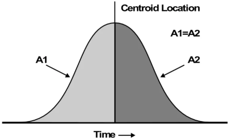
Centroided Peaks
Calculating the centroid of a peak converts peak distribution values into a single value of m/z and intensity that represents the peak. Centroided data collected in profile mode simplifies the data and reduces the file size. Centroided data provides more accurate peak assignment and reduces the amount of data, but it also removes the information about the peak shape.
The centroid algorithm converts peaks to single values by using an intensity weighted average to calculate the center of gravity of the peak. The output of the algorithm is a list of peaks with parameters, as shown in Table 5-1.
Data is automatically calculated as a centroid when added to a library or when a search is conducted.
Calculate the Centroid of a Peak
1. Select a pane containing a spectrum.Calculating the centroid of the peak changes the appearance of the existing graph. To compare the result with the original data, make a copy of the graph before calculating the centroid.
2. Click Explore > Centroid.
Table 5-1 Peak Parameters
Parameter Definition
Centroid Value The value of the centroided data in units of mass or time. Intensity The intensity of each peak in cps.
Qualitative Data Analysis
Figure 5-2 Analyte Centroid Location
Data Analysis
Users can open files containing existing data or data that is currently being acquired. All
experiment-related data can also be viewed in tabular form. The table pane consists of two tabs, the Data List tab and the Peak List tab.The Data List tab contains experiment-related information, such as acquisition time and scan intensity. The Peak List tab displays peak-related information such as peak height, peak area, and baseline type.
Total Ion Chromatogram
A Total Ion Chromatogram (TIC) is created by summing the intensity contributions of all ions from a series of mass scans. Users can use the TIC to view an entire data set in a single pane. It consists of the summed intensities of all ions in a scan plotted against time in a chromatographic pane. If the data contains results from multiple experiments, individual TICs (Total Ion
Chromatograms) for each experiment and another TIC that represents the sum of all
experiments can be created. The preset TIC that represents the sum of all of the experiments is shown with a splitter tool below the center of the x-axis.
Extracted Ion Chromatogram
An Extracted Ion Chromatogram (XIC) is an extracted ion chromatogram created by taking intensity values at a single, discrete mass value, or a mass range from a series of mass spectral scans. It shows the behavior of a given mass, or mass range, as a function of time. The intensity of the ion, or the summed intensities of all ions in a given range, is plotted in a chromatographic pane.
Base Peak Chromatogram
A Base Peak Chromatogram (BPC) displays the intensity of the most intense ion in every scan as a function of scan number or retention time. It is useful in instances where the TIC is so dominated by noise that there is a large offset and chromatographic peaks are hard to distinguish. It is also helps to distinguish between co-eluting components. BPCs only be generated from single period, single experiment data.
A1
A1=A2
Time
A2 Centroid Location
The graph uses two colors, alternating each time the mass of the base peak changes. The color changes are maintained when the data is manipulated by scrolling or zooming. For information about selecting the colors used in the graph, refer to the Help.
Extracted Wavelength Chromatogram
An Extracted Wavelength Chromatogram (XWC) is a wavelength chromatogram created by taking intensity values at a single wavelength, or by the sum of the absorbance for a range of several wavelengths
Diode Array Detector
Users can view the Diode Array Detector (DAD) spectrum for a single point in time, or for a range of time as a Total Wavelength Chromatogram.
Total Wavelength Chromatogram
A Total Wavelength Chromatogram (TWC) is a less commonly used chromatogram. It displays the total absorbance (mAU) as a function of time. The TWC provides a way of viewing an entire data set in a single pane. It consists of the summed absorbances of all ions in a scan plotted against time in a chromatographic pane. If the data contains results from multiple experiments, individual TWCs for each experiment and another TWC that represents the sum of all
experiments can be created.
Overlay Graphs
Two or more sets of data can be visually compared by overlaying graphs created by similar methods. Each individual spectrum is distinguished by the color of its trace. For full scan data, this allows users to visualize the differences between several sample spectra.
If one or more panes are chosen, then each XIC will appear in a separate pane.
1. Select the first pane to be overlaid. 2. Click Explore > Overlay.
3. Click in the second pane.
The graphs are overlaid showing the two traces in different colors.
Tip! To overlay fewer than four graphs in the same pane, press Ctrl + right-click in a pane and then click Appearance Options. In the Appearance Options dialog, Multiple Graph Options tab, select Yes for the Overlay Multiple Panes fields for
Spectrum and Chromatogram.
Tip! To view a color-coded list of the overlaid graphs, right-click the title bar of the pane.
Qualitative Data Analysis
Cycle Between Overlaid Graphs
1. Select a pane that contains overlaid graphs. 2. Click Explore > Cycle Overlays.
The display changes so that the next graph in sequence is shown in the foreground.
Sum Overlays
If two or more graphs overlaid are overlaid, users can sum the graphs to get a new trace. Each point on the new trace is the sum of the points from the graphs. Summing several overlays of similar data type can make subsequent processing operations easier and faster. For example, users can overlay several XICs, sum them, and then smooth the summed overlay to remove noise.
Summing overlays is similar to generating a TIC with the benefit of being able to choose which graphs to overlay. For example, if ten experiments are being viewed, the TIC will add all ten experiments together. If overlays are summed, then users have the option of adding only nine of the ten overlaid graphs. This procedure can be used if the data collected in the one experiment is just noise.
1. Overlay the graphs that are to be summed. 2. Click Explore > Sum Overlays.
The overlaid graphs are added together.
Graphs Labels
Graphs can be customized using the preset style for labels on graphs and chromatograms. Users can select the fonts to use for peak and axis labels, and the colors to use for the traces. Users can also add axis labels and the type of label and precision for the peaks.
Add Captions to a Graph
Use captions to label peaks of interest or significant points on the graph. When a caption is placed beside a peak, the caption stays with the peak when the graph is zoomed in or out. Captions also stay with the original sample when users navigate between samples in a data file. A caption contains one line of text, with a maximum of 128 characters.
1. In the spectrum, right-click, and then click Add Caption. The Add Caption dialog opens.
2. In the Caption box, type the text.
3. To change the size and style of the caption, click Font. 4. To place the caption, click OK.
Tip! If the position of the caption is not satisfactory, then drag the caption to a different position. The caption stays in the same place relative to the x- and y-axes when the graph is zoomed in or out. To edit or delete the caption, right-click the caption and then click the appropriate command.
Add Text to a Graph
Use text to add multiple lines of information to a graph. Unlike captions, which are associated with a specific peak and move with it as the graph is zoomed, text labels remain in their original location as the graph is zoomed. They do not stay with the original sample when users navigate between samples in a data file.
1. In the graph, right-click and then click Add User Text. The Add User Text dialog opens.
2. In the User Text field, type the text.
3. To center the text, select the Center Text check box. 4. To change the size and style of the caption, click Font. 5. To insert the text, click OK.
Compound Database
The compound database stores information about compounds, including optimization
specifications. Use the compound database when there is a large numbers of samples and a large number of compounds need to be optimized quickly. The Compound Database window stores optimized conditions for compounds that can be retrieved to run samples.
Contour Plots
A Contour Plot is a color-coded plot of a complete data set that uses color to represent a third dimension in the plot. In a Contour Plot of a TIC, the x-axis represents retention time or scan number, the y-axis represents mass, and the color represents the intensity of the data at that point. In a Contour Plot of a TWC for DAD data, the x-axis represents retention time or scan number, the y-axis represents wavelength, and the color represents absorbance. The Contour Plot is a post-acquisition tool that does not function in a real-time scan acquisition.
Color is the third axis in Contour Plot, and it represents either intensity or absorbance. Users can change the high and low intensity or absorbance values in Contour Plot using the control
triangles on the color bar above the Contour Plot. The percentage parameters at the top of the Contour Plot pane indicate the values held by the low and high sliders. The actual values are based on a percentage of the maximum intensity or absorbance within the selected area. The value is shown in the top right corner of the Contour Plot pane.
The controls shown in Figure 5-3 change the colors in a Contour Plot.
Tip! If the position of the text is not satisfactory, then drag the text to a different position. To edit or delete the text, right-click the text and then choose the appropriate command.
Note: The Contour Plot does not support MI or MRM scans, but it does support DAD scans.
Qualitative Data Analysis
Figure 5-3 Buttons Controlling Contour Plot Colors
Users can define the colors on a Contour Plot graph to provide better contrast and display data specifications according to their needs. For example, setting the intensity/wavelength and changing the color of the values for Below Low Data and Above High Data can eliminate background noise in a Contour Plot.
The Below Low Data and Above High Data buttons shrink and expand on the color bar if the slider controls are moved. When the contour plot colors are changed, the new colors become the preset colors for all subsequent graphs.
View a Contour Plot
A Contour Plot can be viewed only after acquisition. Users can view a Contour Plot from TIC, XIC, TWC, or XWC graphs. TICs and XICs are available for all .wiff data files. TWCs and XWCs are available only for data acquired by a DAD.
1. In Explore mode, open a data file as a TIC, XIC, TWC, or XWC graph.
2. Highlight the range to be viewed in the Contour Plot. If a selection is not made, the entire range is viewed.
3. Click Explore > Show > Show Contour Plot.
A Contour Plot of the selected area opens in a separate pane.
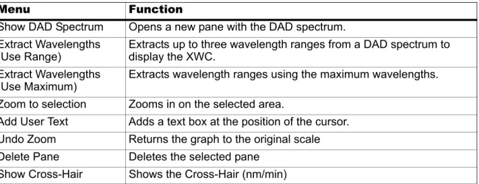
Select an Area in a Contour Plot
To zoom in on a particular selection, or view the corresponding mass spectrum for that selection, do one of the following:
Table 5-2 Right-Click Menu for Contour Plot Panes
Menu Function
Show DAD Spectrum Opens a new pane with the DAD spectrum. Extract Wavelengths
(Use Range) Extracts up to three wavelength ranges from a DAD spectrum to display the XWC. Extract Wavelengths
(Use Maximum) Extracts wavelength ranges using the maximum wavelengths. Zoom to selection Zooms in on the selected area.
Add User Text Adds a text box at the position of the cursor. Undo Zoom Returns the graph to the original scale Delete Pane Deletes the selected pane
• To select a standard area within a box, drag the pointer to create a box around an area in the Contour Plot.
• To make a vertical selection, press Ctrl and drag the pointer vertically. • To make a horizontal selection, press the space bar and drag the pointer
horizontally.
Set the Intensity and Absorbance in a Contour Plot
• Do one of the following:• To set the low intensity/absorbance value in a Contour Plot, from the color bar above the Contour Plot, drag the left triangular slider to the required position. Contour Plot automatically adjusts the color of values below the setting to indicate they are outside the range.
• To set the high intensity/absorbance value in a Contour Plot, from the color bar above the Contour Plot, drag the right triangular slider to the required position. The Contour Plot automatically adjusts the color of values above the setting to indicate they are outside the range.
Change Colors in a Contour Plot
1. In the Contour Plot pane, click one of the color buttons. The Color dialog opens.
2. Click a color. 3. Click OK.
The graph changes to reflect the color change.
Dynamic Background Subtraction Algorithm
Dynamic Background Subtraction™ algorithm improves detection of precursor ions in an IDA (Information Dependant Acquisition) experiment. When the algorithm is activated, IDA uses a spectrum that has been background subtracted to select the ion of interest for MS/MS analysis, as opposed to selecting the precursor from the survey spectrum directly. Because this process takes place during LC analysis, the algorithm enables detection of species as their signal increases in intensity, therefore focusing on detection and analysis of the precursor ions on the rising portion of the LC peak, up to the top of the LC peaks (maximum intensity).
Fragment Interpretation
The Fragment Interpretation tool helps the user interpret MS/MS data. Given the chemical structure of a molecule, this tool can generate a list of theoretical fragment masses from single
Tip! By using the Define Custom Colors palette, users can create customized colors for use in a Contour Plot.
Qualitative Data Analysis non-cyclic bond cleavage of that molecular structure. The tool can then match the theoretical list with peaks in the current mass spectrum.
The Fragment Interpretation Tool generates a list of theoretical fragment masses from single, non-cyclic bond cleavage of a molecular structure. The molecular structure can be created in a third-party drawing program and then saved as a .mol file. Fragment Interpretation displays the theoretical fragments in the fragment list and compares the fragment masses to peaks in the mass spectrum. Peaks above the threshold intensity and within the user-defined mass tolerance (maximum 2 amu) of fragment masses are considered matched and appear in bold text in the fragment list.
• Precursor Ion • Neutral Loss • Q1 Multiple Ion • Q3 Multiple Ion
• Multiple Reaction Monitoring (MRM)
Connect the Fragment Interpretation Tool to a
Spectrum
When a single, non-cyclic bond in the molecular structure is selected, the Fragment
Interpretation tool highlights the two fragments created when the bond is cleaved and matching peaks in the connected spectrum are displayed.
If multiple spectrum panes are being viewed, then the Fragment Interpretation tool connects to the active spectrum. If the data file contains more than one sample, then the Fragment
Interpretation tool connects to the active spectrum.
If a spectrum is open when the Fragment Interpretation tool is opened, then the active panel links to the open spectrum automatically.
1. Click Explore > Show > Show Fragment Interpretation Tool.
2. From the lower right corner of the Fragment Interpretation pane, click the connect button.
The pointer changes to the connecting tool.
3. Click the spectrum graph that is to be connected to the Fragment Interpretation tool. The connected graph indicator in the lower left corner contains the name of the graph connected to the Fragment Interpretation pane. The connection is broken when either the graph or Fragment Interpretation is closed. If the connected .wiff file has more than one sample, the Fragment Interpretation pane updates automatically as users scroll through the samples.
Match Fragments with Peaks
1. Click Explore > Show > Show Fragment Interpretation Tool.
2. With a .mol file in the Fragment Interpretation pane, select a cell in the Fragment List that is shown in bold.
In the spectrum, the software highlights the matching spectral peak in the color selected under the Options tab. In the molecular structure, the bond is highlighted. 3. If a row that has more than one matching fragment is clicked, the spectral peak that
is closest to its monoisotopic mass is highlighted in the mass spectrum in the color specified in the Options tab.
Select a Bond in a Molecular Structure
1. Click Explore > Show > Show Fragment Interpretation Tool.
2. With a .mol file opened in the Fragment Interpretation pane, click a single, non-cyclic bond in the molecular structure.
The two resulting fragments appear as highlights in the fragment list. The masses of the two fragments appear on either side of the bond.
If a spectrum is connected, then the Fragment Interpretation tool displays any matching peaks in the graph. If a fragment in the list is selected and the fragment is matched to a peak, then the Fragment Interpretation window zooms in on that peak.
View Isotopes
The Fragment Interpretation tool can display the theoretical isotopic distribution for a peak matching a fragment in the fragment list.
1. Click Explore > Show > Show Fragment Interpretation Tool. 2. In the Fragment Interpretation pane, click the Options tab. 3. Select the Show Isotopes check box.
4. Click Apply.
5. In the fragment list, select a fragment that matches a peak.
The isotopic distribution for matched peaks is shown in the spectrum.
Display a Formula Difference in a Spectrum
The formula and monoisotopic mass difference between two related hypothetical fragments can be displayed. The formula difference is shown when two peaks are selected. The formula and monoisotopic mass difference is shown when two fragments are selected, or two single, non-cyclic bonds.
1. Click a fragment peak.
2. Press the Shift key and then click another fragment peak.
If the formula difference is equal to a fragment from the fragment list, the fragment highlights in the list. Otherwise, the formula difference between the matching fragments of the peaks is shown in a message box.