New Features in JMP 9

(1)

JMP, A Business Unit of SAS SAS Campus Drive

Cary, NC 27513

“The real voyage of discovery consists not in seeking new landscapes, but in having new eyes.” Marcel Proust

New Features in JMP 9

(2)

The correct bibliographic citation for this manual is as follows: SAS Institute Inc. 2010. New Features in JMP® 9. Cary, NC: SAS Institute Inc.

New Features in JMP® 9

For a hard-copy book: No part of this publication may be reproduced, stored in a retrieval system, or transmitted, in any form or by any means, electronic, mechanical, photocopying, or otherwise, without the prior written permission of the publisher, SAS Institute Inc.

For a Web download or e-book: Your use of this publication shall be governed by the terms established by the vendor at the time you acquire this publication.

U.S. Government Restricted Rights Notice: Use, duplication, or disclosure of this software and related documentation by the U.S. government is subject to the Agreement with SAS Institute and the restrictions set forth in FAR 52.227-19, Commercial Computer Software-Restricted Rights (June 1987). SAS Institute Inc., SAS Campus Drive, Cary, North Carolina 27513.

1st printing, February 2010 2nd printing, April 2010 3rd printing, May 2010 4th printing, October 2010

JMP®, SAS® and all other SAS Institute Inc. product or service names are registered trademarks or trademarks of SAS Institute Inc. in the USA and other countries. ® indicates USA registration. Other brand and product names are registered trademarks or trademarks of their respective companies.

(3)

New Features in JMP 9

New Windows Environment . . . 1

Home Window . . . 2

Window Arrangement Options . . . 2

View the Associated Data Table . . . 3

Preview and Open Reports . . . 4

Switch between Windows . . . 5

Show and Hide Menus . . . 5

Menu and Toolbar Customization . . . 5

Additional Updates in the New Windows Environment . . . 6

Other Windows Updates . . . 6

New Platforms . . . 7

Degradation . . . 8

Neural . . . 8

Data Tables . . . 9

General Table Operations . . . 9

Importing and Exporting Data . . . 11

Data Filter . . . 11

Columns . . . 12

Column Info Window . . . 13

Rows . . . 14 Summary . . . 14 Subset . . . 14 Join . . . 14 Update . . . 15 Tabulate . . . 15 Formula Editor . . . 15 Graph Platforms . . . 16 Graph Builder . . . 16 Bubble Plot . . . 18 Cell Plot . . . 18 Tree Map . . . 18

(4)

ii Scatterplot Matrix . . . 19 Variability/Gauge Chart . . . . 19 Profilers . . . 20 Contour Plot . . . 21 Analysis Platforms . . . 21 Distribution . . . 21 Clustering . . . 22 Discriminant . . . 24 Fit Life by X . . . 24 Fit Y by X . . . 26 Life Distribution . . . 28 Fit Model . . . 29 Multivariate . . . 34 Partition . . . 34 Principal Components . . . 35 Matched Pairs . . . 35 Time Series . . . 35 Recurrence Analysis . . . 36 Survival . . . 36 Nonlinear . . . 37 Categorical . . . 37

Design of Experiments (DOE) . . . 39

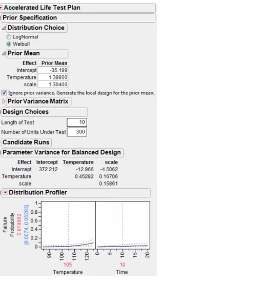
Accelerated Life Test Design . . . 40

Sample Size and Power . . . 40

Graphics and Display . . . 41

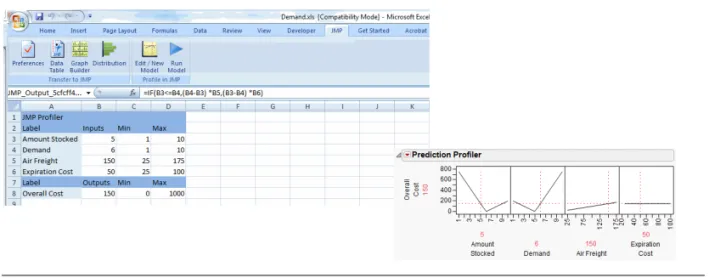
Microsoft Excel Profiler . . . 44

JMP Scripting Language . . . 45

Work with Windows and Files . . . 45

Work with Data Tables . . . 47

Preferences, Path Variables, and Environment Variables . . . 49

Work with the Log . . . 51

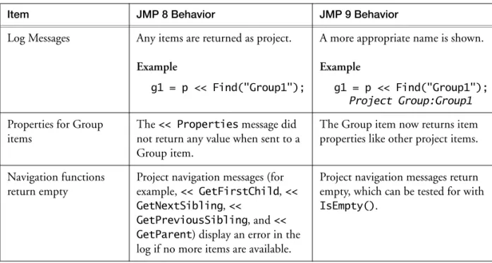
Project Scripting . . . 51

Formula Editor Functions . . . 53

Display Box Functions . . . 54

Updates to JSL Functions . . . 57

Working with R . . . 58

(5)

Add-Ins . . . 60

Projects . . . 60

Preferences . . . 60

Object Scripting Index . . . 62

(6)

(7)

What’s New in JMP

JMP 9 provides major updates to the Microsoft Windows interface and new connections to Microsoft Excel and R. This version also lets you display your data on geographic maps or custom maps, such as an office floorplan.

A new edition of the software, JMP Pro, adds features designed for high-end analytics users. These users have large volumes of data or a need for data mining and predictive modeling.

Important new features include the following:

• a completely revamped Windows environment • two new platforms: Degradation and Neural • the Microsoft Excel add-in

• customized add-in support • Graph Builder enhancements • interface to R

• graphics and display options

• Design of Experiments (DOE) options and the new Accelerated Life Test Design platform

Quick tips for finding the new features are provided here. Refer to the documentation for information about the more complex options.

Note: Features that are available only in JMP Pro, Version 9, are marked as such.

New Windows Environment

On Windows, windows are now free floating and are no longer attached to a parent window. This design works well with multiple monitors, because each window moves independently.

When you first open JMP 9, the new Home Window appears instead of the JMP Starter. To quickly show

the Home Window at any point, click the JMP Home Window button ( ) in the lower right corner of

most JMP windows.

You can change the default window to be either the Home Window, the JMP Starter window, or the JMP Window List. Go to File > Preferences > General, and choose the option from the Initial JMP

Windowlist.

This section describes the features of the new Windows environment and other Windows updates. For details, see the Using JMP book.

(8)

2 New Features in JMP 9

New Windows Environment

Home Window

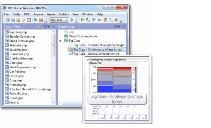
JMP’s new Home Window provides quick access to all open JMP windows and files that you recently

opened through the File menu or Open button. You can open or close windows quickly in the Home

Window rather than manipulate the windows individually.

The Home Window also lets you see a preview of an open report. Place your cursor over a report in the Window List to see the preview.

Figure 1 Report Preview from the Home Window

Window Arrangement Options

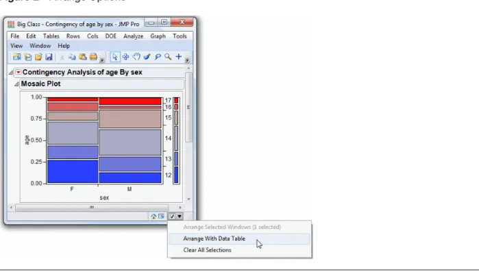
You can now arrange multiple windows side-by-side. This feature is particularly helpful when you have generated several graphs from a data table.

• To see a data table next to the corresponding report window, select the arrow in the bottom right corner of the report window and then select Arrange with Data Table.

• To see multiple windows side-by-side, select the check box in each window. Select the arrow and then

select Arrange Selected Windows.

(9)

Figure 2 Arrange Options

View the Associated Data Table

In a report window, view the data table associated with a report by clicking on the View Associated Data button (Figure 3).

(10)

Preview and Open Reports

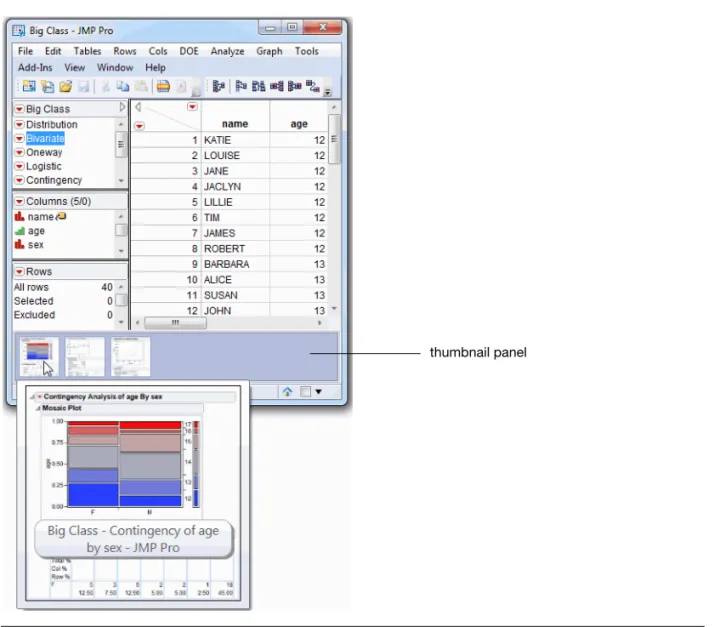
A preview of a data table’s open reports appears in the thumbnail panel, located below the data table (Figure 4). Place your cursor over the thumbnail, and the preview appears, and then double-click on a report to work with it. To see additional options, such as arranging reports with their data table, right-click the thumbnail.

Figure 4 Thumbnail Panel Options

The thumbnail panel appears by default. To hide the panel, select File > Preferences > Windows Specific

and then deselect Show the thumbnail panel in data table windows.

(11)

Switch between Windows

To switch between windows, hold down CTRL and press the TAB key. A preview of each report window appears. Release the keys to open the previewed window.

Show and Hide Menus

In report windows and journals, JMP hides the menu bar by default. Show the menu bar in a specific window by doing one of the following:

• Pressing the ALT key.

• Placing the cursor over the menu strip at the top of the window (Figure 5). • Clicking the menu strip.

If you would rather always see the menu bar, change the auto-hide preference. Select File > Preferences > Windows Specific, and then select Never from the Auto-hide menu and toolbarslist. You can also choose an option to always hide the menu bar regardless of the window size.

Figure 5 Hidden Menu Bar

Menu and Toolbar Customization

The menus and toolbars are customizable on Windows. This feature has been updated significantly in JMP 9.

• The menu editor is a separate window rather than a docked list.

• You can modify menus and toolbars for specific users (such as the current user or all users) or in a JMP add-in.

• You can specify the translation for each button and tooltip.

• JMP 9 lets you quickly hide a menu, toolbar, or button.

To customize menus or toolbars, select View > Customize > Menus and Toolbars and make your changes.

(12)

Additional Updates in the New Windows Environment

• To close JMP and all open windows, hold down the CTRL key and press Q.

• When you close all JMP windows manually, the default window (Home Window, JMP Starter window,

or the JMP Window List) appears. When you close the default window, JMP closes.

• To move a toolbar to the left, right, or bottom of the JMP window, right-click the toolbar and select Location.

• The Log now opens in a separate window. You can also modify the Preferences so that the Log opens

whenever text is added to it, when JMP opens, or only when you explicitly open the Log. Select File > Preferences > Windows Specific > Open the JMP Log window.

• The menus on the menu bar change depending on the window type. For example, the Edit, Cols,

Rows, and Tools menus only appear on windows where you need those options.

• In narrow windows, JMP wraps the main menu so that you can see all menus. You can also choose to

show only the menus that fit in narrow windows. Select File > Preferences > Windows Specific and

deselect Wrap the main menu in narrow windows.

Other Windows Updates

Customize Menu Has Been Moved

The Customize menu has moved from the Edit menu to the View menu. JMP 8 Menus

If custom menus and toolbars (.jmpmenu) are found from JMP 8, JMP 9 attempts to save the

corresponding .jmpcust file and apply the customizations to JMP 9. If there are problems applying a menu or toolbar customization file, an alert window appears. All details are then written to the JMP Log. File_Edit Toolbar Update

The File_Edit toolbar now includes the button for opening the Data Filter window. The Print button on this toolbar has been removed.

Windows Metafile Support

JMP 9 supports the Enhanced Metafile (EMF) graphic formats (including EMF+) to provide the best visual experience.

(13)

Tool Windows Remain in Place

Certain tool windows (such as Data Filter, the Legend window, and the Find and Replace window) remain on top of the windows to which they are attached.

Save Reports and Journals as PDF

You can now save reports and journals as PDF documents. The PDF format is a file type in the Save As window.

New Print Preview Buttons

The following buttons have been added to the File > Print Preview window:

• The Page Setup button opens the Page Setup window, where you specify margins and scale your document.

• The Change Page Orientation button switches between portrait and landscape layouts. • The Show Margins button lets you see the current margins.

• The Shrink One Page button reduces the output size by one page each time it is pressed. More of the report then fits on one printed page.

• The Restore Scale button reverts the output size to the original page size. This button only works after you shrink a page.

New Platforms

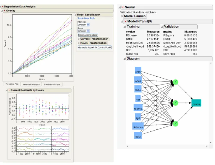
JMP 9 contains two new platforms: Degradation and Neural. Examples of Degradation and Neural reports are shown in Figure 6.

Note that the Neural platform replaces the Neural Net platform and adds significant improvements. For details about the Degradation platform, see the Quality and Reliability Methods book. See the Modeling and Multivariate Methods book for details about the Neural platform.

(14)

New Platforms

Figure 6 Examples of Reports from the New Degradation and Neural Platforms

Degradation

The Degradation platform is available on the Analyze > Reliability and Survival menu. You use this platform to analyze product degradation (or deterioration) over time and to anticipate product quality in the future. Data can be analyzed from both non-destructive (repeated measures or stability analysis) and destructive testing.

Neural

Note: Some of these features are available only in JMP Pro, Version 9.

The Neural platform replaces the Neural Net platform. You can still access the Neural Net platform using

the JMP Scripting Language (JSL) command Neural Net(). To access the new Neural platform, select

(15)

The Neural platform contains significant enhancements. Some of the enhancements include: • the ability to cross validate data based on a validation column

• the option to fit both 1- and 2-layer neural nets • the ability to transform covariates

• three different activation functions

• richer diagnostics, including several measures of fit and diagnostic plots

• the ability to fit multiple responses simultaneously for both continuous and categorical responses • improved handling of missing values. The platform can create a category for missing values of both

continuous and categorical covariates. • the ability to fit boosted neural nets

The Neural platform supports one and two layer, fully connected multilayer perceptron neural networks with activation functions that can be hyperbolic tangent, linear, or Gaussian (exp(-.5*x^2) ). Arbitrary mixtures of continuous and categorical inputs and responses can be modeled.

Data Tables

This section describes the new data table features. For details, see the Using JMP book except where noted.

General Table Operations

Edit Table Property/Script Window

The Script window in a table property lets you define and run a script. This window is no longer modal, so you can keep it open and work with other JMP windows at the same time. You can now run a script or a portion of a script from this window. To run the script, do one of the following:

• Hold down CTRL and press R on Windows (or hold down COMMAND and press R on Macintosh).

• Click the Run button in the Script window.

The window also now has a Save button that lets you save the script without closing the window so that you can continue to work.

Enhanced Numeric Formatting

Data tables support the following new numeric formatting:

• The yyyyQq format returns the four-digit year, the letter “Q,” and the one-digit quarter. To assign the format to a column of data, double-click the column heading and select Format > Date > yyyyQq. To assign the format to an axis, double-click the axis in a graph and select Format > Date > yyyyQq.

• You can use a comma as a thousands separator in numeric formats. The check box is not selected by

default. To use the thousands separator, select the Use thousands separator (,) check box in the Column Info window.

(16)

Data Tables

Manage the Table Grid

You can now hide the data table grid like you can hide the table panels. Hiding the grid hides all data but still shows the properties, scripts, table variables, column names, and row information.

To close the data table grid, click the disclosure icon in the data table panel next to the table name. Copy the Table Script

You can copy the script to reproduce the data table and then paste it into a Script window. To copy a table script, click the red triangle icon in the data table panel next to the table name, and then select Copy Table Script.

Add Encrypted Scripts to a Data Table

You can now encrypt a script that is in a data table. See the Scripting Guide book for directions. Copy and Paste Scripts and Variables in a Data Table

You can now copy and paste scripts and variables that are saved to a data table from the table panel. Select the Copy and Paste commands in the Edit menu. (The Copy and Paste commands are also available in the red triangle menu.)

Undo/Redo Multiple Times

Data tables now support multiple undos and redos. This command works for most modifications to the data table. Changes that do not affect the data cannot be reversed, such as the following:

• all row states operations

• role assignments

JMP does not undo individual data table actions that are sent through a JSL command. (A single JSL command empties the entire data table’s undo stack, not just the previous action.)

The Undo command is also now on the Edit menu.

The new Redo command reverses the previous undo.

Color Cells

You can select a background color for cells in the data table grid using one of the following methods: • Select the color for individual cells by right-clicking the column heading or an individual cell and

selecting Color Cells.

• Color entire rows by their row state. Right-click the row number area and then select Color Rows by

Row State. From then on, the rows are shaded with the color that you assign to the rows.

• Color the column with the Value Colors or Color Gradient property. Double-click the column and

select Column Properties > Value Colors or Color Gradient. Then select the theme from the Color Theme list. When you select the Color by Cell Value check box, the cells in the table are then colored by the color theme. If the option is deselected (which is the default), the colors apply only to the values in the graphs.

(17)

Importing and Exporting Data

Import SPSS Data

You can now import SPSS data that is in a single-byte character set (SBCS). JMP maintains value labels, variable labels, and missing value codes defined in the SPSS file. SPSS is also a file type in the Open Data File window.

SPSS can assign certain values in a variable to be treated as missing for analyses. Now numeric missing value coding is supported when importing SPSS data into JMP.

To specify missing values in a column, select Column Properties > Missing Value Codes and enter the values that should be considered missing.

Import HTML Tables into JMP Data Tables

(Windows only) You can open a Web page in JMP that contains tables and import the tables into JMP data tables.

First, select File > Internet Open, enter the Uniform Resource Locator (URL), select Web page in the Open As list, and then click OK. The page opens in JMP’s browser.

Then, select File > Import Table as Data Table in JMP’s browser. The tables in the Web page are listed. Select one or more tables to convert to JMP data tables.

Wide Range of Character Encodings Supported During Text File Import

• The new preference called Open Text File Charset controls the character encoding for imported text files. This option is on the General page of the Preferences.

• The JSL Open() function now accepts an optional argument that immediately follows the filename

to specify the character encoding.

Data Filter

“And” and “Or” Selections

The Data Filter window has two buttons, And ( ) and Or ( ), to add filter columns. And restricts the selection, while Or extends the selection. The initial window has only the And button. After you select criteria, both the And and Or buttons are available.

Auto Clear

The new Auto clear check box on the Data Filter window lets you select values from one variable at a time. If you want to select values from multiple variables at the same time, deselect the Auto clear check box. Save and Restore Current Row States

A new check box called Save and restore current row states is available in the Data Filter window. This option restores the current row states when the Data Filter window is closed.

(18)

Data Tables Float the Window

A new preference called Use Floating Window controls where the Data Filter window appears after you

generate a report. Select this option in the Data Filter window’s red triangle menu to attach the Data Filter window to the data table. When you click on the data table, the Data Filter window remains on top of the table. Otherwise, the window moves behind the table when you click in the table. (This preference is selected by default.)

To change this preference, select Preferences > Tables and select or deselect Use a Floating Window for Data Filters.

Select Missing

The Select Missing option for a continuous filter column lets you select missing values for that column. If the option is selected, missing values are treated as one category. The specified interval is treated as the other category joined by an OR. If you select a sub-range and select the Select Missing option, then all the rows in the range, including those with missing values, are selected. If you select the Select Missing option and do not select a range, then only rows with missing values are selected.

Columns

Compress Selected Columns

A new command on the Cols menu compresses selected columns as follows:

• In character columns with fewer than 255 unique values, the List Check property is added to the

column.

• In numeric columns, data is compressed to 1-byte, 2-byte, or 4-byte integers when possible.

• A numeric column with non-integer values can also be compressed if there are fewer than 255 unique

values. In this case, the List Check property is added to the column.

To compress columns, select the columns, and then select Cols > Compress Selected Columns.

Fill Columns with Data

The Fill command now supports multiple columns. You can add either a repeating sequence of data or a continuation of values. The pattern that you select in the Fill menu applies to all selected columns. To see the fill options, right-click the cells that contain the values to repeat and select Fill.

Random Indicator

The new Random Indicator option fills a column with random values. This option initializes the data to three values (0, 1, 2) in the specified proportions. To exclude a value, type 0 next to Proportion.

To see the Random Indicator option, double-click on a new empty column and select Random from the

(19)

Color Gradient and Value Colors

You assign the new Color Gradient column property to a continuous column, just as you assign the Value Colors property to nominal or ordinal columns. You can assign the color properties to any column except for row state columns.

To see these color properties, double-click on a column and select Column Properties > Color Gradient or Value Colors.

Copy and Paste Column Properties

You can copy all of the Column Properties for a given column and paste them into another column. Right-click the column heading and select Copy Column Properties. To paste these properties onto

another column, right-click the column heading and select Paste Column Properties.

Recode Script

In the Recode command, there is a fourth menu option called Script. This option creates a new script called Recode in the data table. You can apply this script to perform recoding in-place. If you add more recodes later, the script updates (assuming that you select Script as the destination). You can also apply this script later to new data and then copy the script to other data tables. Running the Recode script from your own scripts is also an option.

Access Column Properties from the Column Right-Click Menu

When you right-click a column heading, there is a new command called Column Properties. This

command lets you quickly select column properties. Previously, you had to right-click, select Column Info, and then select the column property.

Columns Filter

The Select Columns list in most analysis and graph launch windows lets you quickly select columns using the specified criteria (such as columns that only contain continuous data). The platforms that do not support the filter are as follows:

• Fit Model, Fit Parametric Survival, Fit Proportional Hazards

• Choice

To see the column filters, open a launch window (other than those specified above) and select a filter from the Select Columns red triangle menu.

Column Info Window

Missing Value Codes Option

In the Column Properties list, the new option called Missing Value Codes lets you add column values that should be treated as missing. For example, sometimes the value 99 is a placeholder to represent missing values, or sometimes several values are used to represent different types of missing values.

(20)

Data Tables Initialize Data

When you are creating a new column, the Initialize Data option can be set to Today. This feature is useful only with the Date or Time formats.

Rows

Select Dominant Command

The Select Dominant command now lets you select high or low values for each column instead of selecting all high values or all low values for all the selected columns.

To change this setting, select Rows > Row Selection > Select Dominant, and select one or more columns. Then select any column's check box to search for high values, or deselect any column's check box to search for low values.

Summary

Expanded Values when Dragging and Dropping Columns

When you drag and drop columns from the summary table to the source table, the values are expanded in the source table, as if they were matched by grouping columns. This is also true for BY group tables, where the values are pasted to the rows of the corresponding group.

Create Unlinked Summary Tables

You can now specify that a new summary table is not linked to the original data table. The Summary window has a new check box, Link to original data table, which is selected by default.

Subset

Create Subset Tables Based on the Values in a Column

You can now create subset data tables based on the values of one or more columns. The new option called Subset By is available in the Subset window. For example, if you select a column with two levels, two data tables are created. Each table contains the rows for one of the levels of the original column. Note that you can use Subset By with the other options in the Subset window.

Join

Maintain Order While Joining Tables

The new Join window option called Preserve main table order maintains the order of the original data table in the joined table. Otherwise, JMP sorts by the matching columns.

(21)

Update

Select Columns to Add for Updated Tables

You can now add none, some, or all columns that exist in the update table (but not in the original table) to the original table.

To see this feature, select Tables > Update in the table that you want to update. Select the original table’s name, and then do one of the following:

• Select All to add all columns from the new table to the original table.

• Select Selected to add only columns that you are selected in the new table to the original table. • Select None if you do not want to add any additional columns from the new table to the original table.

Tabulate

Missing Value Codes Supported

Missing value codes for grouping columns are supported. The list of values in the column property Missing Value Codes is treated as missing for the purpose of categorization.

To see this feature, double-click on a column and select Column Properties. New Statistics

Two new statistics have been added to the statistics list in the Tabulate window: Row % and Col %. To see these statistics, select Tables > Tabulate.

New Content Supported

The main table area now accepts dropped statistics. Continuous columns are accepted as analysis columns. Delete Items from the Table

When you drag an existing item, such as a statistic keyword, from the table and drop it away from the table, that item is deleted.

Formula Editor

Automatically Fill Match Using Your Data

The Conditional > Match list in the Formula Editor has two new options:

• When you select Add Match Arguments from Data, clauses that correspond to all of the levels in your

data are added automatically.

(22)

Graph Platforms

Note: To add the clauses automatically, you can also hold down the SHIFT key when inserting a Match operator around a column.

New Date Function

The Quarter(date) function returns a quarter value in the range 1 to 4.

Graph Platforms

This section describes the new graph features. For details, see the Basic Analysis and Graphing book.

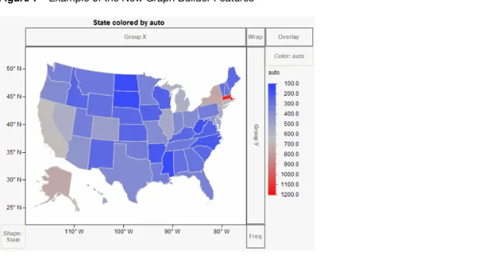
Figure 7 Example of the New Graph Builder Features

Graph Builder

New Zones and Map Support

Two new zones in Graph Builder add color and geographical boundaries to maps:

• The Shape zone assigns geographical boundaries to a map based on variables in the data table. The shape value determines the x and y axes.

Boundaries such as U.S. state names, world countries, Canadian provinces, and Japanese prefectures are installed with JMP. You can also create your own boundaries (whether geographical or otherwise) and specify them as Map Role column properties in the data table.

(23)

• The Color zone applies a color to geographical boundaries. The categorical or continuous color theme selected in your Preferences is applied to each boundary.

Dual Y Axes

To add a y axis on the right side of the graph, drag two or more variables into the left Y drop zone. Then right-click, select Move Right, and select which variable to move to the right y axis.

You cannot drag and drop a right y axis. Instead, right-click and select Move Left or Remove. On the right y axis, the graph contextual menu marks some items as (right). This notation indicates items that are associated with right-hand y variables.

Lock Gradient Scales

The Lock Scales option prevents axis scales and gradient legend scales from automatically adjusting when you filter data. This feature is helpful when you are filtering data over an animation.

To select this option, create a graph in Graph Builder and select Lock Scales from the red triangle menu. Sampling for Large Data Tables

You can now work with a subset of the data table in Graph Builder as you experiment with different options. Then you can switch to the whole data table for the final visualization.

From the Graph Builder red triangle menu, select Sampling and then enter the sample number that you

want to work with. When you want to see the graph for the entire data table, select Sampling again and type 0.

Density Contours

You can now specify the number of density contour levels. This feature is particularly helpful when you want to see patterns in a graph darkened by thousands of data points.

Custom Color Scales and Gradients

There is a gradient color theme legend for continuous color variables in Graph Builder, which allows further customization of how a color theme is applied to data. See “Custom Color Scales and Gradients,” p. 42 for details about the new color features.

Error Bars and Confidence Intervals

Line, Bar, and Points elements in Graph Builder can now show error bars when the Summary Statistic is Mean. The error bars are slightly offset to reduce overstriking. A footer note indicates what type of error bars are in use. To see the error bar option, right-click the graph and select Error Bars from the Line, Bar, or Points option.

(24)

Graph Platforms Frequency Variables

A new drop zone under the Group Y area supports a frequency (or Weight) variable. The Histogram, Mosaic, Contour (density) elements use frequency variables for counts. Line, Bar, and Points elements use frequency variables for summary statistics. Box plots use frequency variables for quantiles, and the fit of the Smoother (or spline) is also affected.

Bubble Plot

No Labels

A new option called No Labels lets you select bubbles without having the labels shown. This is useful for identifying trails without seeing the labels. If both the No Labels and All Labels options are selected, the All Labels option prevails.

Click the Bubble Plot red triangle icon to see these options. Time Label Placement

You can now control the placement of the time variable label by clicking and dragging.

Cell Plot

Custom Color Scales and Gradients

The new custom color scale and gradient feature is available in Cell Plot. See “Custom Color Scales and Gradients,” p. 42 for details about the new color features.

Arrange Plots

If you specify an X, Grouping variable in the launch window, the new Arrange Plots option appears in the red triangle menu. This option lets you specify the number of plots to put on the same row before the next row is created. If you want the maximum across, just enter a large number greater than the number of groups.

Tree Map

Tooltip For Subcategories

Place your cursor over a subcategory to see a tooltip that contains the subcategory’s label. Specify the Color Range

You can now specify the range mapped to the color gradient for continuous variables. The default range is the range of the means across the groups. The Color Range option, which appears only for continuous color variables, prompts you to enter two values.

(25)

Scatterplot Matrix

Regression Lines

Simple regression lines are now available. To show regression lines, select Fit Line from the Scatterplot Matrix red triangle menu.

Nonparametric Densities Option Added

The Nonpar Density Contour option has been added to the Scatterplot Matrix menu. The contour shows where most of the points are located and helps distinguish values in a dense structure. Note the following information about this feature:

• Nonparametric density contours use the default bandwidth.

• This feature has not been added to rectangular scatterplot matrices (where the x and y are different variables).

Variability/Gauge Chart

The Quality and Reliability Methods book provides more details about the following new features. Better Detection of Error Variance Heterogeneity

An ANOMV simulation method now tests for variance heterogeneity in Variability. This comes from a permutation simulation method discussed in the following reference:

Wludyka, Peter, and Sa, Ping (2004) “A robust I-Sample analysis of means type randomization test for variances for unbalanced designs”, Journal of Statistical Computation and Simulation, 74:10, 701-726. You can also set the random seed to get the same results each time you run a heterogeneity of variance test. Before selecting Heterogeneity of Variance Tests in the Variability red triangle menu, hold down the

CTRL and SHIFT keys. Select Heterogeneity of Variance Tests from the Variability Gauge red triangle

menu, and then enter the random seed. Historical Mean for Gauge R&R

A new option to enter the Historical Mean has been added to the Gauge R&R window. This optional value should be used only for one-sided tolerance ranges.

To see this option, create a Variability/Gauge chart and select Gauge Studies > Gauge RR from the red triangle menu.

Conformance Rate

A new option appears in the Conformance Report for changing the conforming category. (The

Conformance Report appears only when there are two rating categories.) JMP assumes that one category is associated with conformance, and the other category is associated with nonconformance. You can switch the category associated with conformance.

(26)

Profilers

To see the Conformance Report, create a Variability/Gauge chart that contains two rating categories. In the

Conformance Report red triangle menu, select Change Conforming Category.

Calculate the Escape Rate

The Conformance Report red triangle menu includes an option to calculate the escape rate. The escape rate is the probability of a miss (flagging a nonconforming part as a conforming part) times the probability that the process produces a nonconforming part. You must enter the probability that the process will produce a nonconforming part.

Change Alpha Levels

You can now change the default alpha level of 0.05 in the launch window. To see this feature, select Graph > Variability/Gauge and click on Specify Alpha.

Profilers

Specify Maximization Options with JSL

You can now specify the following maximization options using JSL:

• Number of Trips

• Maximum Cycles

• Convergence Tolerance

• Save Iterations to a log data table

• Use Legacy Optimizer

See the JMP Object Scripting Index (available in the Help menu) for details about scripting maximization options.

Contour Profiler

You can now change the line color for each response. Right-click a response term in the color legend, and select a color from the color palette. Save the command as a JSL script with the (<<YColors(...) )

command.

The Contour Profiler now uses the Spec Limits of Target LSL and USL as initial values for the Current, Lo Limit, and High Limit respectively.

Simulation Experiments

In the Simulation Experiment window, you can now select which factors you want to include in the experiment.

(27)

Simulator: New Options

There are two new random factors features:

• The External command lets you sample from any column in the source data table or from any column in a different data table.

• The Aligned command applies only to the External and Sample options. When selected on two or more factors, this feature forces the Simulator to choose values from the same row, so that the correlation structure across the columns is preserved.

Column Properties: Expanding Formulas

There is now a way to prevent formulas from being expanded in the Profiler platform. If the value of the Expand Formula column property is zero, then the formulas are not expanded.

To see this feature, double-click the column and select Other from the Column Properties list. Type Expand Formula, click OK, and then type 0 in the Expand Formula window.

Contour Plot

In contour plots, you can show points with missing y values. In the red triangle menu, select Show Missing Data Points. The missing data points are marked with black circles by default, just like the non-missing data points.

Analysis Platforms

This section describes the new analysis platform features. Details about the new features are covered in the Modeling and Multivariate Methods, Quality and Reliability Methods, or Basic Analysis and Graphing books as noted.

Distribution

The Basic Analysis and Graphing book includes details about the new Distribution features. Histograms Only

The Distribution launch window has a new option called Histograms Only. When you select this option,

the Distribution report excludes the following reports:

• Quantiles and Moments reports for continuous variables

• Frequencies reports for nominal and ordinal variables

• Outlier box plots

(28)

Analysis Platforms

Normal Mixture Fitting Options

Normal Mixture fitting options have been added to the Continuous Fit menu on the red triangle menu for distributions of continuous variables. You can select Normal 2 Mixture or Normal 3 Mixture for two or three clusters. Or you can select Other and enter the number of clusters.

Export Histograms as Flash (.SWF) Files

You can export histograms as Flash (.SWF) files that you view with the Adobe Flash Player. Interactive features, such as highlighting bars and adjusting the axes, are available. For details, visit http://

www.jmp.com/support/swfhelp/en/histogram.shtml.

Clustering

The Modeling and Multivariate Methods book includes details about the new Clustering features.

K-Means Clustering

The following new features are available:

• You can run several clusterings, and all are shown in the report. All K-Means clustering options are available on the red triangle menu for each cluster.

• The new multivariate normal mixtures method is available.

• Projected normal contour ellipsoids are shown on biplots.

• Scatterplot Matrix is now available, and it shows projected normal contour ellipsoids. • The Control Panel has a Declutter button for identifying multivariate outliers.

• The command formerly called Simulate Mixtures is now called Simulate Clusters and works on all

clustering methods. It also supports transformations. The following features have been removed:

• The Centers role in the Cluster launch window to specify a grouping variable to define cluster centers. • The Seed with Selected Rows option on the red triangle menu.

Updated Algorithm for K-Means Normal Mixtures Clustering

For K-Means normal mixture clustering, previous versions of JMP used a variation of the Newton-Raphson algorithm. JMP 9 has moved to a more stable algorithm, the expectation-maximization (EM) algorithm. JMP 9 uses a Bayesian regularized version of the EM algorithm, which allows JMP to smoothly handle cases where the covariance matrix is singular.

(29)

Save Cluster Formulas

For the K-Means Clustering, Self Organizing Map, Robust Normal Mixtures, and Normal Mixtures methods, there is a new option to save cluster formulas. Saving cluster formulas creates a column with a formula to evaluate which cluster the row belongs to.

To set this option, select Save Cluster Formula in the K Means red triangle menu.

Hierarchical Clustering Distance Matrices

The new Distance Matrix feature is more visible and specific. A new option, Data is distance matrix, prompts you to specify a subset of objects to cluster. You can still omit the column specification like in JMP 8.

When you analyze distance matrix data, you need to specify the label of the column containing the column names of the other columns. To specify the Label of the column that contains the other columns’ names, select Data is distance matrix in the launch window, and then assign a variable to Label.

There are also two new options:

• Save Distance Matrix creates a new data table that contains the distance matrix. • Get Distance Matrix returns the matrix.

To create a new data table that contains the distance matrix, create a hierarchical cluster report and select Save Distance Matrix from the red triangle menu.

Clustering with Distance Matrices supports two-way clustering and heat maps. Zoom into Dendrograms

You can now zoom in to see just the selected rows in two ways:

• Double-click on a cluster.

• Select a cluster and then select Zoom to Selected Rows from the Hierarchical Clustering red triangle menu.

To see the whole dendrogram again, select Release Zoom from the Hierarchical Clustering red triangle menu.

Reduced Influence of Outliers

For hierarchical cluster heat maps, JMP chooses the mean as the middle. JMP then divides up the low and high parts of the range with the mean in the middle. This prevents bad clustering caused by a single extreme outlier.

(30)

Analysis Platforms Positioning Option

There is a new option on the Hierarchical Clustering red triangle menu item called Positioning. This option lets you select the placement and position of many parts of the dendrogram as follows: • Row Dendrogram Position: select Right or Left

• Row Label Position: select Right or Left

• Row More Position: select Right or Left (for color maps) • Column Dendrogram Position: select Above or Below • Column Label Position: select Above or Below Other New Options

Many other new options are available for Hierarchical Clustering in the red triangle menu: • Show Dendrogram turns the dendrogram on and off.

• Show NCluster Handle turns the diamond indicator in the dendrogram on and off.

• Parallel Coord Plots saves the cluster ID in the data table. JMP launches the Parallel Plot platform using that cluster ID column to produce a parallel plot for each cluster.

• Pivot on Selected Cluster interchanges the two clusters underneath the selected cluster. There is also a line in the distance graph that shows the current number of clusters.

Add Variables to the Cell Plot

You can now add additional variables to the cell plot. To select this option, select More Color Map Columns from the Hierarchical Clustering red triangle menu.

Discriminant

The Modeling and Multivariate Methods book includes details about the new Discriminant features. Indicator for Excluded Rows

When using holdback sets to evaluate prediction accuracy, an indicator column now shows if any rows are excluded.

Fit Life by X

(31)

Custom Estimate

Based on a fitted distribution, Custom Estimate creates tables of estimates along with confidence intervals of failure probabilities and quantiles. Both Wald and profile likelihood intervals are supported. To see this feature, click on the report’s Custom Estimation tab.

Support for Simultaneous Confidence Bands

In the Nonparametric Overlay plot, simultaneous confidence bands are supported for the Kaplan-Meier estimate. To see this feature, select the Interval Type, which can be Simultaneous or Pointwise. Lines of Individual Group Fit

The Nonparametric Overlay plot now draws lines of individual group fit for the specified distributions. To see this feature, create a Fit Life by X graph and view the Nonparametric Overlay report.

New Relationships

The Reciprocal, Square Root, and Box-Cox relationships are available.

To see these options, select Analyze > Reliability and Survival > Fit Life by X and select the Relationship list. If you select Reciprocal or Square Root, the x axis of Scatterplot is scaled so that the quantile lines are straight. Previously, the x axis was linearly scaled.

Transformation for the X Variable in the Scatterplot

For the Arrhenius Celsius, Arrhenius Fahrenheit, Arrhenius Kelvin, Log, and Logit transformation, the x axis is scaled so that quantile lines are straight. Previously, the x axis was linearly scaled.

To see these options, select Analyze > Reliability and Survival > Fit Life by X and select one of the preceding relationships from the Relationship list.

Box-Cox Transformation and Likelihood Profile Plot

If you enter the initial lambda value in the Fit Life by X launch window, the sensitivity of likelihood versus the lambda appears in the Sensitivity report.

To see this feature, create a Fit Life by X graph with the Box-Cox relationship and the initial lambda value. Save Residuals

You can now save residuals in a Cox-Snell Residual P-P Plot by selecting Save Residuals from the Cox-Snell Residual P-P Plot red triangle menu.

(32)

Analysis Platforms

Fit Y by X

The Basic Analysis and Graphing book includes details about the new Fit Y by X features.

Logistic

Save Probability Formula is now available for Logistic in Fit Y by X You can now save the probability formula into the data table.

To see this feature, select Save Probability Formula from the report’s red triangle menu.

Oneway

Exact Tests

Note: This feature is available only in JMP Pro, Version 9. The following exact tests are now available:

• Kolmogorov Smirnov Test

• Median Test

• Van der Waerden Test

• Wilcoxon Rank Sum Test

To run these tests, select Nonparametric > Exact Test in the Oneway red triangle menu and then select the test.

Compare Groups Using Nonparametric Multiple Comparisons

You can now compare groups using nonparametric multiple comparisons. To see this feature, select Nonparametric > Nonparametric Multiple Comparisons from the Oneway red triangle menu. Select Comparison Circles

If you have comparison circles, you can now use the JSL Select Group command to select a particular

circle. The Object Scripting Index (OSI) includes details about this command. (The OSI is available in the

JMP Help menu.)

Analysis of Means Methods

The Analysis of Means Methods menu has been added to the Oneway red triangle menu. This feature lets you compare group means or test for unequal variances using various methods.

(33)

Bivariate

New Residual Plots

The following are new plots: Actual by Predicted, Residual by Row, and Residual Normal Quantile. The Residual by Predicted plot has interactive histogram borders.

To see these features, select Fit Line from the Bivariate red triangle menu. Then select Plot Residuals from the Linear Fit red triangle menu.

New Options for Nonpar Density Fits

Three new options have been added to the Quantile Density Contours menu:

• Contour Lines provides the ability to turn off the lines when you only want a fill.

• Contour Fill fills the space between contours with color density corresponding to the contour.

If grouping is used, the grouping color and transparency (or opaqueness) corresponding to the quantile curves is used. Otherwise, it is colored by its surrounding 10% contour line.

• Select Points by Density lets you enter a low and high probability range for the selection of points. To see these options, select Quantile Density Contours from the Bivariate red triangle menu.

Contingency

Cochran Armitage Trend Test

This option tests for trends in binomial proportions across levels of a single variable. This test is appropriate only when one variable has two levels.

To see this feature, click the red triangle icon on the Contingency Analysis report. Exact Agreement Statistic

Note: This feature is available only in JMP Pro, Version 9.

You can now run an exact test for the Kappa statistic and test agreement between variables. This option is available only when the two variables have the same levels.

Exact Cochran Armitage Trend Test

This option performs the exact version of the Cochran Armitage Trend Test. The test is available only when one of the variables has two levels.

(34)

Analysis Platforms

Cumulative Cell Statistics Added

Four new cell statistics have been added to the Contingency Table menu, as follows: • Col Cum (Cumulative Column) and Col Cum %

• Row Cum (Cumulative Row) and Row Cum %

These statistics are particularly relevant for ordinal variables where you want to see the percent at or below for each level.

To see these options, click the red triangle icon in the Contingency Table report. Analysis of Means for Proportions Option Added

The Analysis of Means for Proportions option has been added to the Contingency platform. This option is available only for data that has a binomial response.

The normal approximation to the binomial distribution is used. A warning message appears if the sample sizes are not large enough to use the normal approximation to the binomial distribution. The report includes a graph and a report with the group proportions, lower and upper limits, and whether the group proportion exceeds one of the limits.

To see this option, click the red triangle icon on the Contingency Table report. Measures of Association Option Added

The Measures of Association option has been added to the Contingency Analysis red triangle menu. This option produces a report with the following measures: Gamma, Kendall’s Tau-b, Stuart’s Tau-c, Somer Ds, Lambda Asymmetric and Symmetric, Uncertainty Coefficient Asymmetric and Symmetric.

Change the Alpha Level

You can now change the alpha level for all confidence levels in the Contingency platform. Select Set α Level from the Contingency Analysis red triangle menu.

Fisher’s Exact Test

You can now perform a Fisher’s Exact test for a table with more than 2x2 levels.

Life Distribution

The Quality and Reliability Methods book includes details about the new Life Distribution features. Custom Estimate

Custom Estimate creates tables of estimates and confidence intervals of failure probabilities and quantiles based on a fitted distribution. Both Wald and profile likelihood intervals are supported. To see this feature, select Custom Prediction from the Parameter Estimate red triangle menu.

(35)

Support for Simultaneous Confidence Bands

In the Compare Distributions plot, simultaneous confidence bands are supported for the Kaplan-Meier estimate. To see this feature, select Interval Type > Simultaneous or Pointwise from the Life Distribution red triangle menu.

Survival Curves

You can plot the probability of survival curves rather than the probability of failure curves throughout the platform. To see this feature, select Show Survival Curve from the Life Distribution red triangle menu. The curves switch from survival to failure.

Fit Model

The Modeling and Multivariate Methods book includes details about the new Fit Model features.

Least Squares

Covariate Values for Contrast

For Least Squares, Generalized Linear Models, and MANOVA Contrast, you can now specify covariate values for cases when the covariate is involved in the contrast.

Joint Profiler for REML Models

When you have multiple responses for REML models, you can now use the Prediction Profiler to optimize all responses at the same time.

Logistic

Confusion Matrix

The Nominal and Ordinal Logistic reports now have a Confusion Matrix option in the red triangle menu.

Model Assessment Using Training and Validation Sets Note: This feature is available only in JMP Pro, Version 9.

You can now assess models by validation and test sets. To create validation and test sets, specify a validation column in the launch window. The values in that column designate which rows are used for training, validation, and test sets. This option is now available in Partition, Neural, and Fit Model (Nominal Logistic and Stepwise).

(36)

Analysis Platforms

Logistic (Nominal and Ordinal) generates validation and test statistics as Neural does.

• The Validation column can now contain character and numeric values.

• The column is treated as a categorical variable with up to three levels: low level for training (except that Stepwise Least Squares supports K-Fold for more than three levels); second level for validation; and third level for Test Set.

Launch Window

Response Surface Macro Allows Categorical Terms

Categorical terms for the Response Surface effect macro can now be selected in the Fit Model launch window. All the main effects and crosses are produced as usual, but square effects for the categorical terms are avoided.

Change the Alpha Level

You can now change the default alpha level (.05) to any valid number. To see this feature, click the red triangle icon on the Model Specification report in the Fit Model launch window and select Set Alpha Level.

Keep the Launch Window Open

You can now choose to keep the launch window open after you run your analysis. Select the check box next to Keep dialog open in the launch window. Alternatively, you can use the new JSL command Modal Dialog in the fitted window.

In addition, the button on the launch window has been changed from Run Model to Run.

Standard Least Squares

Sum of Squares Error Values Added to the Box-Cox

The Box-Cox Transformation Table of Estimates now contains the SSE values. To see this feature, click the red triangle icon on the Standard Least Squares report and select Factor Profiling > Box Cox Y

Transformation. Select Table of Estimates from the Box Cox Transformations report red triangle menu. The new Sum of Squares Error column is populated with values.

New Options in the Save Columns Menu

Two options have been added to the Save Columns menu for the Standard Least Squares personality:

Mean Confidence Limit Formula and Indiv Confidence Limit Formula.

Alpha specification support has been added to JSL command functionality for all saved confidence limits.

Hold down the SHIFT key and select Mean Confidence Limit Formula or Indiv Confidence Limit

(37)

Inverse Prediction Improvements

Inverse prediction in the Fit Model platform has been improved. For example, these improvements are useful in drug stability analyses.

The following features have been updated:

• Inverse prediction is now specified by term value rather than regression design row value. • Virtually any model is allowed, as long as the term of interest participates linearly in the effects.

This means that it works in situations like Analysis of Covariance with an interaction.

• The window is modal rather than contained in the platform report.

• Inverse prediction supports prediction for all levels of categorical variables as an alternative to specifying single category values.

• Inverse prediction still does not support REML and quadratic terms of interest.

• A new graph is produced with the confidence intervals.

• The Fit Y by X Logistic and Fit Model Nominal Logistic platforms also now support the new Inverse

Prediction facility.

• Inverse prediction now uses a Wald interval if the Fieller interval fails for both sides. • If only one side of the interval fails, it is set to missing (implying infinity).

• Inverse prediction now supports one-sided intervals using combo box specification or through scripting. To see the inverse prediction improvements, create a Fit Model report and select Estimates > Inverse Prediction from the red triangle menu. Enter the Y values to include in the inverse prediction. Overlay LS Means Plots

To further illustrate three-way interactions, multiple overlay LS Means plots now appear in the report window (assuming that your model has a three-way interaction).

Show the Variance Inflation Factor and Confidence Intervals

The Fit Least Squares platform includes two new options on the Preferences menu:

• Show VIF always shows the Variance Inflation Factor (VIF) for the Parameter Estimates report. • Show All Confidence Intervals always shows all of the confidence intervals in the Parameter Estimates

report that might otherwise be hidden. To turn this feature on and off, select or deselect Regression Reports > Show All Confidence Intervals in the report’s red triangle menu.

Save Standard Error Prediction Formula for Split Plot Models

For the split plot models using the REML method, the report menu option to save the standard error prediction formula (STDErr Pred Formula) is now available.

(38)

Analysis Platforms Stepwise

Stepwise Features

The following Stepwise features have been added:

• Stepwise now supports multiple y variables. Each y variable can be modeled separately. To apply actions to all y variables, hold down the CTRL key and click Go.

• Click the Run Model button to generate all test results in the same report window. JMP uses the current model and directly calls the appropriate personality, such as Standard Least Squares or Ordinal Logistic • The fitting statistics have been moved so that they are more easily seen when you fit multiple models.

The statistics are now located directly above the Current Estimates report. To make the model-fitting statistics row more visible in the report when fitting multiple models, right-click the other disclosure buttons and select Close All Like This.

• The response variable name is now located in the title bar for each model and is shown as a separate outline. The title bar is labeled Stepwise Fit for YNAME.

• RMSE is now shown instead of MSE in the model-fitting statistics row, but MSE is available as a hidden column. To see the MSE column, right-click in the model-fitting statistics row and select Columns > MSE.

• New columns have been added to the model-fitting statistics row and include p (the number of

parameters in the model) and BIC (Bayesian Information Criterion).

• The following new stopping rules are available:

– Minimum AIC – Minimum BIC

– Validation RSquare (if a validation column is specified) The old stopping rule (P-value Threshold) is not recommended.

• You can click the radio button for a step to return the model to its previous state in the step history. Model Assessment Using Training and Validation Sets

You can now assess models by validation and test sets. To create validation and test sets, specify a validation column in the launch window. The values in that column designate which rows are used for training, validation, and test sets. This option is now available in Partition, Neural, and Fit Model (Nominal Logistic and Stepwise).

Stepwise generates validation and test statistics as Neural does.

• The Validation column can now contain character and numeric values.

• The column is treated as a categorical variable with up to three levels: low level for training (except that Stepwise Least Squares supports K-Fold for more than three levels); second level for validation; and third level for Test Set.

(39)

You select the Validation column in the launch window. The values in that column designate which rows are used for training, validation, and test sets. For continuous responses, you can use both holdback and K-Fold cross validation. For nominal and ordinal responses, you can use only holdback validation.

On the red triangle menu, the K-Fold Crossvalidation command starts K-Fold at that time using a random selection. Note that once you begin this process, the process is committed and cannot be disabled.

Nominal and Ordinal Logistic

Confidence Intervals Added for Odds Ratios

• In the Nominal Logistic personality, confidence intervals have been added for the odds ratios for two-level responses.

• The Parameter Estimates report now includes a Covariance of Estimates report. This report shows the

variances and covariances of the parameter estimates. Whole Model Test Report Updates

For the Nominal Logistic personality, a new section appears in the Whole Model Test report that includes these columns: Measure, Training, and Definition.

• When you specified a validation set, additional columns appear. The additional column is Validation.

• When there are tied maximums, the misclassification rate contains a message to indicate this. When

there are fitted zero probabilities for events that occur in the validation data, a message appears. For the Nominal and Ordinal Logistic personalities, the Whole Model Test report now includes the corrected Akaike’s Information Criterion (AICc) and the Bayesian Information Criterion (BIC) results.

Proportional Hazard

Risk Ratio Confidence Intervals Added for Nominal and Ordinal Factors

Risk Ratio confidence intervals in the Cox Proportional Hazards model are now calculated for both nominal and ordinal factors. Previously, only confidence intervals for continuous factors were calculated. A report called Covariance of Estimates has also been added to the Parameter Estimates report. This report shows the variances and covariances of the parameter estimates.

Generalized Linear Model

Inverse Prediction and Additional Diagnostic Plots

When you want to predict an x value given a y value and the values of all the other factors, you can now use inverse prediction. To see this feature, create a Generalized Linear Model report. Select Inverse Prediction from the red triangle menu, and then enter the y values to include in the prediction.

(40)

Analysis Platforms

The following diagnostic plots are also new:

• Regression plot shows the responses and the model on the Y axis and the continuous covariate on the

X axis. This plot is available only when you specify one continuous predictor and no more than one categorical predictor. The Regression Plot is generated by default.

To hide the plot, select Diagnostic Plots > Regression Plot from the Generalized Linear Model red triangle menu.

• Linear Predictor plot shows the linear model plotted on the Y axis and the continuous covariate on the X axis. The inverse link function transformed responses are overlaid. This plot is available only when there is one continuous predictor and no more than one categorical predictor. To see this feature, select Diagnostic Plots > Linear Predictor Plot from the Generalized Linear Model red triangle menu.

Multivariate

The Modeling and Multivariate Methods book includes details about the new Multivariate features. Multi-Threaded Estimation Methods

Rowwise and pairwise estimation methods are now multithreaded.

To see this feature, select Analyze > Multivariate > Multivariate Methods > Multivariate and select Row-wise or Pairwise from the Estimation Method list.

Partition

The Modeling and Multivariate Methods book includes details about the new Partition features. Bootstrap Forest and Boosted Tree Options

The new Bootstrap Forest and Boosted Tree options fit many Partition models and combine them to generate more accurate predictions than a single Partition model can predict.

To see these features, select Analyze > Modeling > Partition and select Bootstrap Forest or Boosted Tree from the Method list. After you click OK, enter the Bootstrap Forest or Boosted Tree specifications. Model Assessment Using Training and Validation Sets

You can now assess models by validation and test sets. To create validation and test sets, select Analyze > Modeling > Partition and do one of the following:

• Specify a Validation column in the launch window. The values in that column designate which rows are

used for training, validation, and test sets.

(41)

You can also select Show Fit Details from the red triangle menu to show several measures of fit and a confusion matrix. The confusion matrix is a two-way classification of actual and predicted response. This feature is for categorical responses only.

Principal Components

The Modeling and Multivariate Methods book includes details about the new Principal Components features.

Maximum Likelihood Factor Analysis

You can now choose Maximum Likelihood as the factoring method. This method is from Magnus and Neudecker, Matrix Differential Calculus.

Add Promax For Factor Analysis

Promax is a new oblique rotation method available in factor analysis as a factor rotation method.

Matched Pairs

The Basic Analysis and Graphing book includes details about the new Matched Pairs features. Perform a Sign Test

You can now perform a sign test for matched pairs. This is a nonparametric version of the paired t-test that uses only the sign (positive or negative) of the differences for the test.

To see this feature, select Sign Tests from the Matched Pairs red triangle menu.

Time Series

The Modeling and Multivariate Methods book includes details about the new Time Series features. New ARIMA Model Group Option

You can simultaneously fit a range of ARIMA models. Previously, you could fit only a single model at a time.

Save Prediction Formula Option

Creates a new data table containing the forecast formula, which you can use to forecast future values. To see this feature, click the red triangle icon on the ARIMA Model report and select Save Prediction Formula.