Yi-Ta Wu, Chuan Zhou, Heang-Ping Chan, Chintana Paramagul, Lubomir M. Hadjiiski, and Caroline Plowden Daly
Department of Radiology, University of Michigan, Ann Arbor, Michigan 48109 Julie A. Douglas
Department of Human Genetics, University of Michigan, Ann Arbor, Michigan 48109 Yiheng Zhang, Berkman Sahiner, Jiazheng Shi, and Jun Wei
Department of Radiology, University of Michigan, Ann Arbor, Michigan 48109
共Received 21 January 2009; revised 18 November 2009; accepted for publication 19 November 2009; published 28 December 2009兲
Purpose: Automated detection of breast boundary is one of the fundamental steps for computer-aided analysis of mammograms. In this study, the authors developed a new dynamic multiple thresholding based breast boundary共MTBB兲detection method for digitized mammograms.
Methods: A large data set of 716 screen-film mammograms 共442 CC view and 274 MLO view兲
obtained from consecutive cases of an Institutional Review Board approved project were used. An experienced breast radiologist manually traced the breast boundary on each digitized image using a graphical interface to provide a reference standard. The initial breast boundary共MTBB-Initial兲was obtained by dynamically adapting the threshold to the gray level range in local regions of the breast periphery. The initial breast boundary was then refined by using gradient information from hori-zontal and vertical Sobel filtering to obtain the final breast boundary共MTBB-Final兲. The accuracy of the breast boundary detection algorithm was evaluated by comparison with the reference stan-dard using three performance metrics: The Hausdorff distance共HDist兲, the average minimum Eu-clidean distance共AMinDist兲, and the area overlap measure共AOM兲.
Results: In comparison with the authors’ previously developed gradient-based breast boundary
共GBB兲algorithm, it was found that 68%, 85%, and 94% of images had HDist errors less than 6 pixels共4.8 mm兲for GBB, MTBB-Initial, and MTBB-Final, respectively. 89%, 90%, and 96% of images had AMinDist errors less than 1.5 pixels 共1.2 mm兲 for GBB, Initial, and MTBB-Final, respectively. 96%, 98%, and 99% of images had AOM values larger than 0.9 for GBB, MTBB-Initial, and MTBB-Final, respectively. The improvement by the MTBB-Final method was statistically significant for all the evaluation measures by the Wilcoxon signed rank test
共p⬍0.0001兲.
Conclusions: The MTBB approach that combined dynamic multiple thresholding and gradient information provided better performance than the breast boundary detection algorithm that mainly used gradient information. © 2010 American Association of Physicists in Medicine.
关DOI:10.1118/1.3273062兴
Key words: breast boundary detection, computer-aided detection, mammogram, multiple thresh-olding
I. INTRODUCTION
It has been shown that computer-aided detection共CAD兲for mammography can increase breast cancer detection sensitiv-ity by radiologists both in the laboratory and in clinical practice.1–6Automated detection of breast boundary is one of the fundamental steps for computer-aided analysis of mam-mograms, including detection of breast lesions,7,8estimation of breast density,9prediction and correlation of mass location in multiview mammograms,10–12 and other image analysis applications.13,14 Breast boundary determination therefore plays an important role in CAD systems.
The breast region of digitized mammograms generally has lower x-ray exposure, and thus higher brightness, than the
background outside the breast. However, the breast region cannot be correctly separated from the background by a single threshold value because of the variation in x-ray ex-posure along the boundary. In addition, the markers and la-bels in the image background may be connected to the breast if they are placed too close to the breast or if the breast is large. Most breast boundary detection algorithms9,15–20share a common approach, in which an initial breast area is ob-tained by analyzing the gray level histogram and the final breast boundary is determined by a subsequent refinement procedure. These algorithms may fail if the initial breast boundary 共MTBB-Initial兲 deviates too far from the true boundary such that the refinement procedure is misled to the wrong direction.
Bick et al.15 classified the image pixels into potential breast pixels and other background pixels by a modified his-togram analysis, and the final breast boundary was derived by region growing and morphological filtering. Ojala et al.17 obtained the initial breast boundary by adaptive histogram thresholding and morphological filtering. The inner stroma edge was extracted by the thresholding method of Otsu,21 and the next boundary point was predicted by analyzing the Euclidean distance between the inner stroma edge and the outer initial confirmed portion. Three different smoothing procedures, Fourier transform, snake, and B-splines, were used to obtain the final breast boundary. Wirth and Stapinski16 utilized dual thresholding22 to obtain the initial control points. After performing edge enhancement and noise removal, those control points were input to the snake to ob-tain the final breast boundary. Ferrari et al.18determined the initial breast boundary based on the following three steps. First, the image contrast was enhanced using the logarithmic operator. Second, the breast region was thresholded based on the Lloyd–Max quantizer. Third, the binary morphological opening operator was adopted to reduce the noises along the initial breast boundary. In the refinement stage, the final breast boundary was derived by the adaptive active deform-able contour model. Sun et al.19 obtained the initial breast boundary by a combination of adaptive thresholding and connected-component analysis, and then determined the ini-tial confirmed portion of the breast boundary by a greedy range selection procedure. They derived the final breast boundary based on the assumption of Euclidean distance constraint between the initial confirmed portion and the stroma edge computed via bimodal histogram analysis. Raba et al.20determined the initial breast boundary by an adaptive histogram analysis, and then obtained the final boundary by a region growing approach. A fair comparison would require testing the different algorithms with a common data set. Due to the lack of details for some of these published methods, it would be very difficult to implement the methods correctly and compare the accuracy of our and their algorithms in our data set.
We have previously developed a breast boundary detec-tion method by using a gradient-based breast boundary
共GBB兲technique to search for the breast boundary.9The im-age background was estimated initially by searching for the largest peak in the gray level histogram. After excluding the background from the breast region, an initial edge was de-rived by a line-by-line gradient analysis from the top to the bottom of the image. The tracking of the breast boundary started from approximately the middle of the breast image and moved upward and downward along the initial boundary. The tracked edges were smoothed to remove noisy fluctua-tions. In most of these methods, the refinement of the breast boundary may fail if the initial breast boundary was too far from the true boundary.
The initial breast boundary therefore plays an important role in a breast boundary detection system. In this study, we developed a new system for automated breast boundary de-tection which estimated the initial breast boundary based on a dynamic multiple thresholding method instead of
histo-gram analysis. The final breast boundary was tracked along the initial breast boundary with refinement of the edge loca-tion by analysis of the gradient informaloca-tion obtained from horizontal and vertical Sobel filtering. The accuracy of the breast boundary detection was evaluated by comparison with an experienced breast radiologist’s manual segmentation. The performance of the new method was also compared to that of our previous method.
II. MATERIALS AND METHODS II.A. Data sets
A data set of 716 screen-film mammograms 共442 CC view and 274 MLO view兲were obtained from 288 consecu-tive cases of an ongoing NIH-supported and Institutional Re-view Board approved genetic study of breast density in women from the Old Order Amish population of Lancaster County, PA.23 The mammograms were digitized with a Lu-miscan laser scanner at a pixel size of 50⫻50 m2 and 12
bits/pixel. The mammograms were first smoothed with a 16⫻16 pixel box filter and subsampled by a factor of 16, resulting in a pixel size of 800⫻800 m2 and an
approxi-mate image size of 225⫻300 pixels. For each mammogram, the breast boundary was manually traced by an experienced Mammography Quality Standards Act 共MQSA兲 radiologist. The radiologist used the windowing function to enhance the breast boundary and outlined the breast boundary with the cursor on a graphical user interface. The radiologist’s seg-mented boundaries were used as reference standard for per-formance evaluation of our method.
II.B. Methods
In order to improve the performance of the breast bound-ary detection system, we developed a new dynamic thresh-olding based method, referred to as the multiple threshthresh-olding breast boundary共MTBB兲detection method. Breast boundary detection is performed in two stages: Initial breast boundary determination and breast boundary refinement. The detailed description for each stage is presented below.
II.B.1. Initial breast boundary determination
As mentioned earlier, the quality of the initial breast boundary is critically important for breast boundary detec-tion. Figure 1shows an example of obtaining several initial breast boundaries by the thresholding approach using differ-ent threshold levels. It is obvious that a single threshold level cannot properly determine the initial breast boundary. For example, in Fig. 1共b兲, the anterior portion of the initial boundary is closed to the real boundary. However, the boundary encloses a large number of background pixels in the top and bottom areas which will mislead the boundary tracking in the refinement procedure. The relatively high x-ray intensity in these regions is caused by scattered radia-tion from the chest wall of the patient. Although the back-ground pixels can be removed by selecting a higher threshold level as shown in Figs.1共c兲–1共g兲, the anterior portion of the initial boundary will then move too far inside the breast as
shown in Figs. 1共f兲 and 1共g兲. In order to obtain the initial breast boundary as close as possible to the true boundary, we have designed a dynamic multiple thresholding method that contains two steps, breast boundary candidate search, and initial breast boundary extraction, as discussed below.
II.B.1.a. Breast boundary candidate search. Figure 2
shows an example of performing the initial breast boundary candidate共IBBC兲search procedure when the breast is on the right side of the mammogram. To initiate the IBBC search, a threshold value h on the image histogram is obtained by the method of Otsu.21 Let LMX _ h be the leftmost x-coordinate of the IBBC at the threshold level h within the middle sec-tion of the image共from about 1/4 to 3/4 along the y dimen-sion of the image兲, as shown in Fig.2共a兲. A threshold level l will start from a lower value than h, e.g., 0.5
*
h, as shown in Fig. 2共b兲 and is gradually increased to remove background pixels, guided by a search criterion described below. At a given threshold l, the leftmost x-coordinate LMX _ l is deter-mined and a rectangular area having a width of2
*
共LMX _ h − LMX _ l兲and centered at LMX _ h is defined in the anterior portion of the breast candidate as shown in Fig.2共c兲. Note that the width of the rectangular area is decreasing when the threshold l increases, and it will become 0 if the threshold l reaches the high threshold level h obtained by the method of Otsu. Within the rectangle, each column of pixels is searched to determine its intersection with the anterior of the breast region that is above the threshold l. If the pixel column intersects the breast region at more than one contigu-ous sections, it indicates that the region boundary is not smooth and unlikely to be the breast boundary. The threshold l will then continue to be increased. Figure 2共d兲shows that the threshold l search procedure is completed since only a single continuous breast region intersects with each pixel column at the anterior of IBBC. This final threshold l is considered to be the starting threshold level in the boundary tracking procedure below.
II.B.1.b. Initial breast boundary extraction. Once the IBBC is obtained in the previous step 关Fig.2共d兲兴, the initial breast boundary can be tracked by evaluating the differences between every two thresholded images at consecutive thresh-old levels as shown in Fig.3. Figures3共a兲and3共b兲show two thresholded images obtained at two consecutive threshold levels. Figure 3共c兲shows the differences 共white pixels兲 be-tween the two thresholded images. The boundary tracking procedure is performed in two parts, the top and bottom por-tion of the breast boundary that were separated by the white dashed line shown in Fig. 3共d兲. The location of the line is determined by the vertical coordinate of the leftmost pixel of the IBBC, which may, but not necessarily, be the nipple. For each portion, a new boundary pixel is found in each iteration at the intersection between the central column of the white region and the gray breast region by comparing the two thresholded images. The boundary pixels found in one of the iterations are marked as gray circles in the example shown in Fig. 3共d兲共pointed by the white arrow兲. Figure4 shows the iterative search of obtaining the MTBB-Initial.
II.B.2. Breast boundary refinement
The refinement procedure of our MTBB detection system tracks the boundary based on the MTBB-Initial and the
gra-FIG. 1. An example of obtaining several initial breast boundaries by the thresholding approach.共a兲The original image with gray levels in range关0,4095兴;
共b兲–共g兲the initial breast boundaries derived in threshold levels 300, 500, 700, 900, 1100, and 1300, respectively.
FIG. 2. An example of performing the initial breast boundary candidate search procedure.共a兲LMX _ h at threshold level h obtained by the Otsu’s method. Although the IBBC seems to be close to the true boundary in the anterior portion, it contains many background pixels in the top and bottom chest wall areas.共b兲The search of a proper threshold level l for boundary tracking will start from a lower value than h and is gradually increased to remove background pixels.共c兲and共d兲illustrate the procedure to search for
l. The white rectangles in 共c兲 and 共d兲 are centered at the fixed location LMX _ h shown in共b兲, and have a width of 2*共LMX _ h − LMX _ l兲 for a given threshold l. The threshold level l is increased after 共c兲since some columns within the rectangular area contain more than one contiguous sec-tion, but stops increasing after共d兲.
dient information. The tracking procedure starts from the same approximately middle point described above 关see ex-ample in Fig.3共d兲兴and moves upward and downward along the initial boundary. The use of the gradient information in the two directions is schematically shown in Fig.5. The gra-dient information was obtained by Sobel filtering in the hori-zontal and vertical directions. The horihori-zontal gradient infor-mation 共vertical Sobel兲 is utilized to track the edges in the ranges between A and B and between A and D. The vertical gradient information 共horizontal Sobel兲 is utilized to track the edges in the ranges between B and C and between D and E. The selection of either the vertical or horizontal gradient is determined based on the slope: If the absolute slope of the tangent to the current boundary position is greater than 1, the horizontal gradient is selected; otherwise, the vertical gradi-ent is selected. An example of a mammogram in Fig. 6共a兲
after vertical and horizontal Sobel filtering is shown in Figs.
6共b兲and6共c兲, respectively.
The gradient information is one of the references in the refinement procedure; therefore, the tracking procedure will be affected if the gradient information of the breast boundary is distorted by that of artifacts along the boundary area. In order to alleviate this problem, in each step of boundary tracking, three predicted points 共Ai, i = 2 , 3 , 4兲 based on the gradient information and four derived points
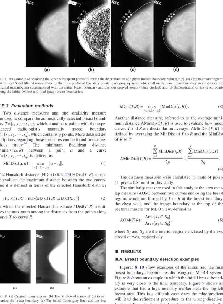
共Bj, j = 1 , 2 , 3 , 4兲 based on the initial breast boundary are estimated as candidates for the next boundary point. Figure7
shows an example of obtaining the seven points for search-ing the next boundary point after a boundary point p共x , y兲is tracked. The two-step strategy for determining the seven points depends on the region where the breast boundary is being tracked. In the regions using the horizontal gradient information共AB and AD in Fig.5兲, the y-coordinates for the seven pixels are first calculated by setting a constant pixel spacing d between each pair of the predicted boundary points and between each pair of the four derived points along the initial breast boundary, i.e., the distances between the y-coordinates of the point pairs 共p , A2兲, 共p , A3兲, and 共p , A4兲 are set to be d, 2d, and 3d, respectively, and those between
共B1, B2兲,共B1, B3兲, and共B1, B4兲to be d, 2d, 3d, respectively. The y-coordinate of B1 is the same as that of p共x , y兲. The
points are spaced upward for the upper portion of the breast boundary共AB in Fig.5兲and spaced downward for the lower portion 共AD in Fig. 5兲 from the last tracked point. The x-coordinates of the three predicted boundary points are de-termined by using the properties of the local horizontal gra-dient information that the gragra-dient at the boundary is usually high and will gradually decrease as the distance from the boundary increases. The x-coordinates of the four derived points are taken to be the x-coordinates of the initial ary points at the corresponding y-coordinates. As the bound-ary tracking proceeds to the regions using the vertical gradi-ent information 共BC and DE in Fig. 5兲, the roles of the x-coordinates and the y-coordinates described above are re-versed.
FIG. 3. An example illustrating the breast boundary tracking procedure.共a兲 and 共b兲The thresholded images in two consecutive threshold levels. 共c兲 Comparison of the two thresholded images by overlapping.共d兲The new breast boundary points are derived by analyzing the differences of the two thresholded images.
FIG. 4. An example of tracking the initial breast boundary by dynamic multiple thresholding.共a兲–共f兲show the iterative tracking of the breast boundary in which the white pixels mark the differences between the two consecutive thresholded images, and the light gray circles共pointed out by the arrows兲are the boundary points obtained in each iteration of increasing the threshold.共g兲The initial breast boundary, MTBB-Initial, is obtained by collecting all the boundary points.
Once the seven subsequent pixels are derived after a tracked boundary point p共x , y兲, two types of slopes will be determined to predict the next boundary point as follows.
Type I Slope: Obtained from the tracked boundary point p共x , y兲 and three predicted points, i.e., the slopes 共angles兲 between lines pA2, pA3, and pA4 and the horizontal line in
Fig.7共b兲. For example, slope = 1 indicates 45° and slope= 0 indicates 0°.
Type II Slope: Obtained from the four pixels on the initial breast boundary, i.e., the slopes共angles兲between lines B1B2, B1B3, and B1B4and the horizontal line in Fig.7共c兲.
The slope between the current tracked boundary point p共x , y兲 and its previous tracked points, referred to as the “previous slope,” is used as a reference to determine the next boundary point. First, the Type I slopes using the three pre-dicted points Ai 共i = 2 , 3 , 4兲 are compared to the previous slope. Since the three predicted points are determined based on the gradient information, it is possible that unreasonable predicted points such as markers near the breast boundary are chosen. Let ThSbe the slope change threshold. If at least one of the three differences between the Type I slopes and the previous slope is smaller than or equal to ThS, the suit-able slope will be determined from Type I slopes according to the minimum difference. Otherwise, if the differences be-tween all three Type I slopes and the previous slope are greater than ThSthe abrupt change in slope may indicate the presence of artifacts and we will search for the next bound-ary point using the Type II slopes. The suitable slope will be considered to be one of the Type II slopes that has the mini-mum difference from the previous slope. Finally, the coordi-nate of the next breast boundary point is determined by choosing a constant distance from the current tracked bound-ary point in the y-coordinate and to calculate the x-coordinate using the “suitable slope” for the regions AB and AD, or correspondingly choosing a constant distance from the x-coordinate followed by calculating the
y-coordinate for the regions BC and DE. The constant dis-tances are chosen to be d, 2d, and 3d when selecting the slopes derived from B1B2, B1B3, and B1B4, respectively,
which are the same distances as those for setting up the pre-dicted or derived points. If the minimum difference between the Type II slopes and the previous slope is greater than ThS, a slope change in ThSis used to determine the next boundary point to avoid sharp direction change in the breast boundary. The constant pixel spacing d and the slope change thresh-old ThSwere determined experimentally. The ranges of these parameters were initially estimated by taking into consider-ation some a priori knowledge of breast boundaries. First, since the slope is changing gradually along the breast bound-ary, the value of the constant pixel spacing should be large enough to avoid an abrupt slope change. For example, if the pixel spacing is too small, e.g., 1 pixel, the tracking proce-dure will be sensitive to noise. The slopes will have large fluctuations and the determination of the next boundary point by comparing the slope differences will be unreliable. Sec-ond, since the breast boundary is smooth, the value of the constant pixel spacing should be small enough to provide adequate sampling of the boundary curve. For example, if the pixel spacing is set to be too large, e.g., 30 pixels, two problems may arise: One is that the slope along the breast boundary may change by a large amount and the use of the previous slope as a guide may not be meaningful, and the other is that the final breast boundary points will be piece-wise linear. Our experiments indicated that a spacing of 3–5 pixels is the best range to perform the refinement procedure when images with 800 m pixel size are used. In this study, we chose d = 3 pixels. Similarly, for the slope change thresh-old ThS, if it is too small, e.g., 1°, the tracking procedure prefers to find a nearly straight line along the breast bound-ary, but the true boundary is curved gradually. On the other hand, if the slope threshold is set to be too large, e.g., 45°, the tracking procedure will allow an abrupt angle change and thus may not be able to avoid a marker or label that overlaps with the breast boundary. Our experiments indicate that 10°– 20° is the best range, and we chose ThS= 0.3共around 17°兲in this study.
FIG. 5. Vertical and horizontal Sobel filtering used in the breast boundary refinement.
(a) (b) (c)
FIG. 6. An example showing 共a兲an original mammogram,共b兲horizontal,
II.B.3. Evaluation methods
Two distance measures and one similarity measure are used to compare the automatically detected breast bound-ary T =兵t1, t2,¯, tp其, which contains p points with the expe-rienced radiologist’s manually traced boundary R =兵r1, r2,¯, rq其, which contains q points. More detailed de-scriptions regarding those measures can be found in our pre-vious study.24 The minimum Euclidean distance MinDist共␣, R兲 between a point ␣ and a curve R =兵r1, r2,¯, rq其is defined as
MinDist共␣,R兲= min i苸兵1,2,¯,q其储␣
− ri储. 共1兲
The Hausdorff distance共HDist兲 共Ref.25兲HDist共T , R兲is used to evaluate the maximum distance between the two curves, and it is defined in terms of the directed Hausdorff distance as
HDist共T,R兲= max兵hDist共T,R兲,hDist共R,T兲其 共2兲 in which the directed Hausdorff distance hDist共T , R兲 identi-fies the maximum among the distances from the points along curve T to curve R,
hDist共T,R兲= max i苸兵1,2,¯,p其兵
MinDist共ti,R兲其. 共3兲 Another distance measure, referred to as the average mini-mum distance AMinDist共T , R兲is used to evaluate how much curves T and R are dissimilar on average. AMinDist共T , R兲is defined by averaging the MinDist of T to R and the MinDist of R to T AMinDist共T,R兲=
兺
i=1p MinDist共ti,R兲 2p +兺
i=1 q MinDist共ri,T兲 2q . 共4兲 The distance measures were calculated in units of pixels共1 pixel= 0.8 mm兲in this study.
The similarity measure used in this study is the area over-lap measure共AOM兲between two curves enclosing the breast region, which are formed by T or R at the breast boundary, the chest wall, and the image boundary at the top of the pectoral muscle for MLO view, defined as
AOM共T,R兲=Area兵ST艚SR其 Area兵ST艛SR其
, 共5兲
where STand SRare the interior regions enclosed by the two closed curves, respectively.
III. RESULTS
III.A. Breast boundary detection examples
Figures 8–10 show examples of the initial and the final breast boundary detection results using our MTBB system. Figure8shows an example in which the initial breast bound-ary is very close to the final boundbound-ary. Figure 9 shows an example that has a high intensity marker near the top-left breast area. This is a difficult case since the edge gradient will lead the refinement procedure to the wrong direction. However, by using the initial breast boundary as a guide, the
FIG. 7. An example of obtaining the seven subsequent points following the determination of a given tracked boundary point p共x , y兲.共a兲Original mammogram;
共b兲vertical Sobel filtered image showing the three predicted boundary points共dark gray squares兲, which fall on the final breast boundary in most cases;共c兲 original mammogram superimposed with the initial breast boundary and the four derived points共white circles兲; and共d兲demonstration of the seven points along the initial共white兲and final共gray兲breast boundaries.
FIG. 8. 共a兲Original mammogram.共b兲The windowed image of共a兲to em-phasize the breast boundary.共c兲The initial共inner gray line兲and the final
final breast boundary tracked by the MTBB algorithm is close to the true boundary. Figure10shows another example containing a low intensity label covering a small section of the anterior breast boundary. Again, the final breast boundary is closer to the true boundary than the initial boundary.
III.B. Performance evaluation
We evaluated the performance of our dynamic MTBB de-tection method in comparison with the radiologist’s manual segmentation. We also compared the performance of MTBB to our previously developed GBB detection approach.9Table
Iand Fig.11show the MTBB method achieved smaller dis-tance errors and slightly larger AOMs than the GBB method. The P-values of two-tailed Wilcoxon signed rank test on the following three comparisons共GBB vs MTBB-Initial兲,关GBB vs final breast boundary共MTBB-Final兲兴, and共MTBB-Initial vs MTBB-Final兲 using the three evaluation measures are shown in TableII. All comparisons show that the improve-ment achieved with our newly developed method 共 MTBB-Final兲is statistically significant.
IV. DISCUSSION
The initial breast boundary plays an important role in the breast boundary detection system since it can lead the track-ing or refinement procedure to avoid artifacts along the breast boundary. Figure 12 shows an example in which a label is in contact with the nipple region. Figure12共a兲shows that the GBB was diverted to the edge of the label 共gray line兲, while the new MTBB method successfully tracked the boundary共white line兲. In this example, the dynamic multiple thresholding method correctly identified the initial breast boundary but the GBB method initially found the edge of the label because of the simple line-by-line search. The subse-quent refinement could not correct for this major error be-cause it deviated too far from the true boundary. For the
(a) Hausdorff Distance (pixels)
0 5 10 15 20 25 Percentage of Images 0 20 40 60 80 MTBB-Final MTBB-Initial GBB
(b) Average Minimum Distance (pixels)
0 1 2 3 4 5 Percentage of Images 0 20 40 60 80 100 MTBB-Final MTBB-Initial GBB
(c) Area Overlap Measure
0.70 0.75 0.80 0.85 0.90 0.95 1.00 Percentage of Images 0 20 40 60 80 100 MTBB-Final MTBB-Initial GBB
FIG. 11. Cumulative counts of the number of images having the perfor-mance measure;共a兲Hausdorff distance and共b兲average minimum Euclidean distance, less than a given value, and共c兲area overlap greater than a given value by comparing the automated breast boundary detection to an MQSA radiologist’s manual segmentation.
(a) (b) (c)
FIG. 9. 共a兲Original mammogram containing a high intensity marker共the LMLO label兲near the top-left boundary.共b兲The windowed image of共a兲to show the breast boundary.共c兲The initial共inner gray line兲and the final共outer white line兲breast boundaries.
(a) (b) (c)
FIG. 10. 共a兲Original mammogram containing a low intensity object 共the shadow of a label兲covering a small section of the left breast boundary.共b兲 The windowed image of 共a兲to show the breast boundary.共c兲The initial
cases without markers or labels along the boundary, the ini-tial breast boundary still serves as an important guide for the tracking procedure, especially in regions where the boundary is closed to the nipple or chest wall. Figure 13 shows an example comparing the GBB method共gray line兲and MTBB-Final共white line兲results. In order to extract the nipple, the GBB method used a lax criterion to search for the edge while tracking the boundary. However, the lax criterion is sensitive to noise and thus GBB found an outer edge, probably due to scattered radiation, around the nipple region. The strong scat-tered radiation near the chest wall caused a similar problem. In these situations, the combined information from the Sobel gradients and the initial breast boundary used in the refine-ment stage of the MTBB method guided the tracking to the correct boundary. These examples demonstrated that the MTBB method can improve the nipple location and shape along the breast boundary. This will likely improve the ac-curacy of automated nipple detection for multiple view analysis.
Our experiences in breast boundary detection indicate that the initial breast boundary has a strong impact on the overall accuracy of breast boundary detection. The complexity of the refinement procedure will likely depend on the difference between the initial breast boundary and the true boundary, i.e., the farther the initial breast boundary is from the true
one, the more complicated techniques and rules may be needed during the refinement process to find the optimal boundary. Many breast boundary detection systems obtain the initial breast boundary by thresholding. However, our study indicated that it is difficult to obtain a reasonable initial boundary by using a simple thresholding approach. In this study, we developed a dynamic multiple thresholding ap-proach to obtain the initial breast boundary. The key steps of our method include共1兲the initial accurate determination of the anterior region of the breast region; 共2兲 the gradual in-crease in the threshold from low to high levels starting from the breast anterior region; 共3兲limiting the search for initial boundary points only within a small breast peripheral region at each level; and共4兲analyzing the differences between two thresholded images at consecutive threshold levels to prevent large change in the boundary direction. The adaptation of the thresholding to the local breast boundary improves the chance that the initial breast boundary is close to the true boundary despite the variation in the x-ray intensity in the breast boundary region. Furthermore, in the refinement pro-cess, the search for the next boundary point is guided by the previously tracked breast boundary direction and the com-parison of multiple boundary point candidates. Both tech-niques reduce the chance of tracking into artifacts at the breast boundary. Because only a small fraction of the mam-mograms will have the problem of artifacts or noise at the breast boundary, the overall improvement in the performance measures over the entire data set by our new breast boundary tracking methods only changed by small fractions. However, this small fraction of problematic cases, for which commonly used boundary detection methods would fail, makes it
diffi-TABLEI. Comparison of automated boundary detection with an experienced
radiologist’s manual segmentation for 716 mammograms.
GBB 共%兲 MTBB-Initial 共%兲 MTBB-Final 共%兲
Percentage of images having HDist
error less than 6 pixels共4.8 mm兲 68 85 94 Percentage of images having
AMinDist error less than 1.5 pixels
共1.2 mm兲 89 90 96
Percentage of images having AOM
values larger than 0.9 96 98 99
TABLEII. The two-tailed P-values of the improvement in the breast bound-ary accuracy estimated from Wilcoxon signed rank test between pairs of the three methods.
HDist AMinDist AOM GBB vs MTBB-Initial ⬍0.0001 ⬍0.0001 0.50 GBB vs MTBB-Final ⬍0.0001 ⬍0.0001 0.0006 MTBB-Initial vs MTBB-Final ⬍0.0001 0.0002 ⬍0.0001 FIG. 12. An example, in which a label is connected to the nipple region,
showing共a兲the GBB共gray line兲and MTBB-Final共white line兲results,共b兲 vertical, and共c兲horizontal gradient information by Sobel filtering. In com-parison to manual segmentation, the AOM, HDist, and AMinDist measures for the GBB boundary were 0.929 and 20.22 pixels, and 1.52 pixels, respec-tively, and those for the MTBB-Final boundary were 0.976 and 2.45 pixels, and 0.32 pixels, respectively.
FIG. 13. An example showing共a兲 the GBB共gray line兲and MTBB-Final
共white line兲results,共b兲vertical, and共c兲horizontal gradient information by Sobel filtering. In comparison to manual segmentation, the AOM, HDist, and AMinDist measures for the GBB boundary were 0.893 and 8.54 pixels, and 1.34 pixels, respectively, and those for the MTBB-Final boundary were 0.969 and 2.24 pixels, and 0.43 pixels, respectively.
CAD systems such as nipple detection, multiview correlation of lesion detection or characterization.12,26–30 The improve-ment achieved by the new method is a step toward full au-tomation of these processes.
The AOM is a commonly used metric for comparison of the agreement between two segmented objects. However, it is well known that AOM does not clearly reveal spurious errors that do not cause a large difference in the segmented object area. For the breast boundary detection problem, one major source of error is the artifacts that cause local devia-tions in the boundary as demonstrated in the examples in Figs.10,12, and13. We therefore chose the Hausdorff dis-tance to measure this type of errors. The average minimum Euclidian distance共AMinDist兲is a commonly used measure of the average distance between two curves that can more specifically than the AOM show the deviation between the boundaries. In addition, the AMinDist provides the average rather than the maximum of the differences and is thus complementary to the Hausdorff distance.
To estimate the intraobserver and interobserver variabili-ties in the manual segmentation, a subset of 50 CC view and 50 MLO view mammograms was randomly selected from the data set of 716 mammograms. The same radiologist共R1兲 who provided the reference standard for the entire data set and a second MQSA radiologist共R2兲were asked to outline the breast boundaries of the subset more than a year after the first segmentation. The radiologists performed the new seg-mentation independently without knowledge of the previous segmentations. The similarity measure, AOM, and distance measures AMinDist and HDist, between pairs of the segmen-tations, denoted by R1共1兲, R1共2兲, and R2, were calculated The intraobserver variability was estimated by the three mea-sures between R1共1兲 and R1共2兲, and the interobserver vari-ability was estimated by the three measures between R1共1兲 and R2 or between R1共2兲and R2, as shown in Fig.14. The intraobserver variation was slightly smaller than the interob-server variations; however, the differences in either the inter-observer or intrainter-observer variations did not achieve statisti-cal significance for these two experienced radiologists, as estimated by the two-tailed P-values of the Wilcoxon signed rank test共TableIII兲. In comparison to the results in Fig.11, the differences between the current 共MTBB兲 and previous
共GBB兲methods are much greater than the interobserver and intraobserver variations, especially for the Hausdorff dis-tance that measures the sporadic large deviations from the reference boundary, which was substantially reduced by the MTBB method.
Our algorithms involve several parameters. We deter-mined these parameters empirically by experimenting with small subsets of the available data set. To evaluate the con-sistency of the algorithm performance in the large data set, we randomly grouped the 716 images by case into two sub-sets, each with 358 images. We calculated the three perfor-mance measures AOM, AMinDist, and HDist, and estimated the significance in their differences between the two subsets using the nonparametric Mann–Whitney test for unpaired data. The two-tailed P-values for the three measures were
0.19, 0.54, and 0.26, respectively. We repeated the same ex-periment with two other different groupings. The two-tailed P-values were 0.54, 0.07, and 0.15, respectively, for the sec-ond grouping and 0.50, 0.42, and 0.61, respectively, for the third grouping. These experiments indicate that there were no significant differences in the performance measures be-tween the random subsets of images. Therefore, although our chosen parameters may not be optimal and the performance was not evaluated in an independent test set, we expect that the parameters used would be reasonably robust because the validation sample size of over 700 used in this study was relatively large. Even if the entire set was used for training, the training performance would approach that of test perfor-mance when the training sample size is sufficiently large.31,32 The breast boundary detection algorithm developed in this (a) Hausdorff Distance (pixels)
0 5 10 15 20 25 Percentage of Images 0 20 40 60 80 R1(1) and R1(2) R1(1) and R2 R1(2) and R2
(b) Average Minimum Distance (pixels)
0 1 2 3 4 5 Percentage of Images 0 20 40 60 80 100 R1(1) and R1(2) R1(1) and R2 R1(2) and R2
(c) Area Overlap Measure
0.70 0.75 0.80 0.85 0.90 0.95 1.00 Percentage of Images 0 20 40 60 80 100 R1(1) and R1(2) R1(1) and R2 R1(2) and R2
FIG. 14. Cumulative counts of the number of images having the
perfor-mance measures;共a兲Hausdorff distance and共b兲average minimum Euclid-ean distance, less than a given value, and共c兲area overlap greater than a given value by comparing the two segmentations R1共1兲and R1共2兲by the first radiologist, and one segmentation R2 by the second radiologist.
study is mainly useful for digitized mammograms. For digi-tal mammograms, the breast laterality and view label is usu-ally shown only on the viewing workstation so that they will not contribute artifacts to breast boundary detection using the digital files. The breast boundaries are also easier to detect, especially in the “for presentation” images. However, screen-film mammography is still commonly used in breast imaging clinics to date and may continue to be a competitive modal-ity in years to come since digital mammography systems are much more expensive and have not been found to be supe-rior to screen-film mammography in all types of breasts.33 Improvement of the CAD methods for screen-film mammog-raphy will continue to be an important area of research. Im-proving the accuracy of breast boundary detection will be the fundamental step in implementing many advanced tech-niques that can enhance CAD performance.
Although our MTBB algorithm can circumvent the prob-lem of markers or other artifacts overlapping with the breast boundary in most of the cases as demonstrated in Figs.9and
10, there are still two cases in which our algorithm failed to exclude the object when the high intensity object happened to be the leftmost point in the initial breast boundary, as shown in an example in Fig. 15. In such cases, the refine-ment procedure would take the object as the starting point and then moved upward and downward along the initial boundary. The marker would therefore not be excluded by the proposed method. We believe this problem may be alle-viated either by designing more intelligent criteria on the
selection of the starting point, or by performing a postpro-cessing procedure to identify unusual shape regions along the breast boundary and refine the boundary locally. Further work is underway to reduce these errors.
V. CONCLUSIONS
Many breast boundary detection systems obtain the breast boundary by first determining an initial boundary which is used to guide the tracking of a final boundary. However, those systems may fail due to errors in the initial boundary. Our MTBB system determines the initial boundary based on dynamic adaptation of the threshold to local regions of the breast periphery. The final boundary is then tracked based on the initial boundary and the gradient information. In com-parison to a gradient-based method, the new method reduces the chances that the detected breast boundary would be mis-led by artifacts and noise along the breast boundary. The new method improved the agreement between the automated de-tected breast boundary and that manually outlined by an ex-perienced breast radiologist, as estimated by three perfor-mance measures, the HDist errors, the AMinDist errors, and the area overlap. Our results demonstrate that the analysis of thresholded images based on dynamic adaptation of thresh-old levels is a robust approach to the detection of breast boundary.
ACKNOWLEDGMENTS
This work is supported by USPHS Grant No. RO1 CA95153. The genetic study of breast density in the Amish population is supported by USPHS Grant No. R01 CA122844 共P.I. Julie Douglas, Ph.D.兲. The content of this article does not necessarily reflect the position of the funding agencies and no official endorsement of any equipment and product of any companies mentioned should be inferred.
a兲Author to whom correspondence should be addressed. Electronic mail:
[email protected]; Telephone: 734-647-8553; Fax: 734-615-5513.
1
H. P. Chan, K. Doi, C. J. Vyborny, R. A. Schmidt, C. E. Metz, K. L. Lam, T. Ogura, Y. Wu, and H. MacMahon, “Improvement in radiologists’ de-tection of clustered microcalcifications on mammograms. The potential of computer-aided diagnosis,”Invest. Radiol.25, 1102–1110共1990兲.
2
L. J. Warren Burhenne, S. A. Wood, C. J. D’Orsi, S. A. Feig, D. B. Kopans, K. F. O’Shaughnessy, E. A. Sickles, L. Tabar, C. J. Vyborny, and R. A. Castellino, “Potential contribution of computer-aided detection to the sensitivity of screening mammography,” Radiology 215, 554–562
共2000兲.
3
T. W. Freer and M. J. Ulissey, “Screening mammography with computer-aided detection: Prospective study of 12,860 patients in a community breast center,”Radiology220, 781–786共2001兲.
4
R. F. Brem, J. K. Baum, M. Lechner, S. Kaplan, S. Souders, L. G. Naul, and J. Hoffmeister, “Improvement in sensitivity of screening mammogra-phy with computer-aided detection: A multi-institutional trial,” AJR, Am. J. Roentgenol. 181, 687–693共2003兲.
5
S. V. Destounis, P. DiNitto, W. Logan-Young, E. Bonaccio, M. L. Zuley, and K. M. Willison, “Can computer-aided detection with double reading of screening mammograms help decrease the false-negative rate? Initial experience,”Radiology232, 578–584共2004兲.
6
M. A. Helvie et al., “Sensitivity of noncommercial computer-aided detec-tion system for mammographic breast cancer detecdetec-tion—A pilot clinical trial,”Radiology231, 208–214共2004兲.
7
N. Petrick, H. P. Chan, B. Sahiner, and M. A. Helvie, “Combined adap-tive enhancement and region-growing segmentation of breast masses on digitized mammograms,”Med. Phys.26, 1642–1654共1999兲.
TABLE III. The two-tailed P-values estimated from the Wilcoxon signed
rank test on the differences in the breast boundaries between pairs of the R1 and R2 segmentations obtained by the three performance measures. R1共1兲 = first outline by R1, R1共2兲= second outline by R1, R2 = outline by R2. The performance measure was calculated relative to each of the radiologist’s segmentations as “reference” shown in column 2.
Reference HDist AMinDist AOM R1共2兲and R1共1兲vs R2 and R1共1兲 R1共1兲 0.09 0.49 0.19 R1共1兲and R1共2兲vs R2 and R1共2兲 R1共2兲 0.10 0.14 0.052 R1共1兲and R2 vs R1共2兲and R2 R2 0.97 0.36 0.61
(a) (b) (c)
FIG. 15. 共a兲Original mammogram containing a high intensity marker.共b兲 The vertical Sobel filtered image of共a兲to show the horizontal gradient information.共c兲The initial共inner gray line兲and the final共outer white line兲 breast boundaries. The marker was considered as the starting point for the refinement procedure so that the final result contained the marker.
son of performance on full-field digital mammograms and digitized film mammograms,” Radiological Society of North America, Program Book, p. 387共2003兲.
9
C. Zhou, H. P. Chan, N. Petrick, M. A. Helvie, M. M. Goodsitt, B. Sahiner, and L. M. Hadjiiski, “Computerized image analysis: Estimation of breast density on mammograms,”Med. Phys.28, 1056–1069共2001兲.
10
L. M. Hadjiiski, B. Sahiner, E. M. Caoili, R. H. Cohan, and H. P. Chan, “Automated detection of ureter abnormalities on multidetector row CT urography,” Proc. SPIE 6144, 1W1–1W7共2006兲.
11
B. Sahiner, N. Petrick, H. P. Chan, S. Paquerault, M. A. Helvie, and L. M. Hadjiiski, “Recognition of lesion correspondence on two mammographic views—A new method of false-positive reduction for computerized mass detection,”Proc. SPIE4322, 649–655共2001兲.
12
S. Paquerault, N. Petrick, H. P. Chan, B. Sahiner, and M. A. Helvie, “Improvement of computerized mass detection on mammograms: Fusion of two-view information,”Med. Phys.29, 238–247共2002兲.
13
C. Zhou, H.-P. Chan, C. Paramagul, M. A. Roubidoux, B. Sahiner, L. M. Hadjiiski, and N. Petrick, “Computerized nipple identification for mul-tiple image analysis in computer-aided diagnosis,”Med. Phys.31, 2871–
2882共2004兲.
14
Y. Zhang, H.-P. Chan, B. Sahiner, Y.-T. Wu, C. Zhou, J. Ge, J. Wei, and L. M. Hadjiiski, “Application of boundary detection information in breast tomosynthesis reconstruction,”Med. Phys.34, 3603–3613共2007兲.
15
U. Bick, M. L. Giger, R. A. Schmidt, R. M. Nishikawa, D. E. Wolverton, and K. Doi, “Automated segmentation of digitized mammograms,”Acad. Radiol.2, 1–9共1995兲.
16
M. A. Wirth and A. Stapinski, “Segmentation of the breast region in mammograms using snakes,” in Proceedings of the First Canadian Con-ference on Computer and Robot Vision, 2004, pp. 385–392共unpublished兲.
17
T. Ojala, J. Nappi, and O. Nevalainen, “Accurate segmentation of the breast region from digitized mammograms,” Comput. Med. Imaging Graph.25, 47–59共2001兲.
18
R. J. Ferrari, R. M. Rangayyan, J. E. L. Desautels, R. A. Borges, and A. F. Frere, “Identification of the breast boundary in mammograms using active contour models,”Med. Biol. Eng. Comput.42, 201–208共2004兲.
19
Y. Sun, J. S. Suri, J. E. L. Desautels, and R. M. Rangayyan, “A new approach for breast skin-line estimation in mammograms,”Pattern Anal. Appl.9, 34–47共2006兲.
20
D. Raba, A. Oliver, J. Marti, M. Peracaula, and J. Espunya, “Breast seg-mentation with pectoral muscle suppression on digital mammograms,” in
Pattern Recognition and Image Analysis, Lecture Notes in Computer
Sci-ence Vol. 3523共Springer, Berlin/Heidelberg, 2005兲, pp. 471–478.
22
P. L. Rosin, “Unimodal thresholding,”Pattern Recogn.34, 2083–2096
共2001兲.
23
J. A. Douglas, M.-H. Roy-Gagnon, C. Zhou, B. D. Mitchell, A. R. Shul-diner, H.-P. Chan, and M. A. Helvie, “Mammographic breast density— Evidence for genetic correlations with established breast cancer risk fac-tors,”Cancer Epidemiol. Biomarkers Prev.17, 3509–3516共2008兲.
24
B. Sahiner, N. Petrick, H. P. Chan, L. M. Hadjiiski, C. Paramagul, M. A. Helvie, and M. N. Gurcan, “Computer-aided characterization of mammo-graphic masses: Accuracy of mass segmentation and its effects on char-acterization,”IEEE Trans. Med. Imaging20, 1275–1284共2001兲.
25
D. P. Huttenlocher, G. A. Klanderman, and W. J. Rucklidge, “Comparing images using the Hausdorff distance,”IEEE Trans. Pattern Anal. Mach. Intell.15, 850–863共1993兲.
26
L. Hadjiiski, H. P. Chan, B. Sahiner, N. Petrick, and M. A. Helvie, “Au-tomated registration of breast lesions in temporal pairs of mammograms for interval change analysis—Local affine transformation for improved localization,”Med. Phys.28, 1070–1079共2001兲.
27
L. Hadjiiski, B. Sahiner, H. P. Chan, N. Petrick, M. A. Helvie, and M. N. Gurcan, “Analysis of temporal change of mammographic features: Computer-aided classification of malignant and benign breast masses,”
Med. Phys.28, 2309–2317共2001兲.
28
J. Wei, B. Sahiner, L. M. Hadjiiski, H.-P. Chan, M. A. Helvie, M. A. Roubidoux, C. Zhou, J. Ge, and Y. Zhang, “Two-view information fusion for improvement of computer-aided detection共CAD兲of breast masses on mammograms,” Proc. SPIE 6144, 241–247共2006兲.
29
Y.-T. Wu, J. Wei, L. M. Hadjiiski, B. Sahiner, C. Zhou, J. Ge, J. Shi, Y. Zhang, and H. P. Chan, “Bilateral analysis based false positive reduction for computer-aided mass detection,”Med. Phys.34, 3334–3344共2007兲.
30
B. Zheng, J. K. Leader, G. S. Abrams, A. H. Lu, L. P. Wallace, G. S. Maitz, and D. Gur, “Multiview-based computer-aided detection scheme for breast masses,”Med. Phys.33, 3135–3143共2006兲.
31
H. P. Chan, B. Sahiner, R. F. Wagner, and N. Petrick, “Classifier design for computer-aided diagnosis: Effects of finite sample size on the mean performance of classical and neural network classifiers,”Med. Phys.26,
2654–2668共1999兲.
32
B. Sahiner, H. P. Chan, and L. Hadjiiski, “Classifier performance predic-tion for computer-aided diagnosis using a limited data set,”Med. Phys. 35, 1559–1570共2008兲.
33
E. D. Pisano, C. Gatsonis, E. Hendrick, and M. Yaffe, “Diagnostic per-formance of digital versus film mammography for breast-cancer screen-ing,”N. Engl. J. Med.353, 1773–1783共2005兲.