Kent Academic Repository
Full text document (pdf)
Copyright & reuse
Content in the Kent Academic Repository is made available for research purposes. Unless otherwise stated all
content is protected by copyright and in the absence of an open licence (eg Creative Commons), permissions
for further reuse of content should be sought from the publisher, author or other copyright holder.
Versions of research
The version in the Kent Academic Repository may differ from the final published version.
Users are advised to check
http://kar.kent.ac.uk
for the status of the paper.
Users should always cite the
published version of record.
Enquiries
For any further enquiries regarding the licence status of this document, please contact:
[email protected]
If you believe this document infringes copyright then please contact the KAR admin team with the take-down
information provided at
http://kar.kent.ac.uk/contact.html
Citation for published version
Gao, Zhifu and Song, Yan and McLoughlin, Ian Vince and Guo, Wu and Dai, Li-Rong (2018)
An Improved Deep Embedding Learning Method for Short Duration Speaker Verification. In:
Interspeech 2018, 2-6 Sept 2018, Hyderabad, India. (In press)
DOI
Link to record in KAR
http://kar.kent.ac.uk/67451/
Document Version
An Improved Deep Embedding Learning Method for Short Duration Speaker
Verification
Zhifu Gao
1, Yan Song
1, Ian McLoughlin
2, Wu Guo
1, Lirong Dai
11
National Engineering Laboratory of Speech and Language Information Processing University of
Science and Technology of China, Hefei, China
2
School of Computing, University of Kent, Medway, UK
[email protected], {songy, lrdai, guowu}@ustc.edu.cn, [email protected]
Abstract
This paper presents an improved deep embedding learn-ing method based on convolutional neural networks (CNN) for short-duration speaker verification (SV). Existing deep learning-based SV methods generally extract frontend embed-dings from a feed-forward deep neural network, in which the long-term speaker characteristics are captured via a pooling op-eration over the input speech. The extracted embeddings are then scored via a backend model, such as Probabilistic Lin-ear Discriminative Analysis (PLDA). Two improvements are proposed for frontend embedding learning based on the CNN structure: (1) Motivated by the WaveNet for speech synthesis, dilated filters are designed to achieve a tradeoff between com-putational efficiency and receptive-filter size; and (2) A novel cross-convolutional-layer pooling method is exploited to cap-ture1st
-order statistics for modelling long-term speaker charac-teristics. Specifically, the activations of one convolutional layer are aggregated with the guidance of the feature maps from the successive layer. To evaluate the effectiveness of our proposed methods, extensive experiments are conducted on the modi-fied female portion of NIST SRE 2010 evaluations, with con-ditions ranging from 10s-10s to 5s-4s. Excellent performance has been achieved on each evaluation condition, significantly outperforming existing SV systems using i-vector and d-vector embeddings.
Index Terms: speaker verification, convolution neural network, dilated convolution, cross-convolutional-layer pooling
1. Introduction
Speaker verification (SV) is the task of determining whether the claimed identity of a speaker matches an enrolled identity, ac-cording to their speech. A typical SV system consists of a fron-tend embedding learning stage and a backend modeling stage. A low-dimensional embedding that is rich in speaker informa-tion is extracted in the frontend learning stage, and the similar-ities between embeddings are computed for verification by the backend modelling stage.
For decades, the most successful SV systems have relied on i-vectors with a PLDA backend [1, 2, 3, 4, 5, 6, 7], which model speaker representations and channel variability in a low-dimensional space. An i-vector is learned through a pipeline of generative modelling, as shown in Section 2. Despite excel-lent performance on long-duration evaluations, the effectiveness of i-vectors degrades dramatically for short-duration record-ings [8, 9].
Several methods based on deep learning have recently been proposed to extract frontend embeddings for short-duration SV [10, 11, 8, 9, 12]. In [10], deep neural networks (DNNs)
were employed to learn speaker embeddings, termed d-vectors. In [12, 8], deep CNNs were exploited to model long-term tem-poral dependencies. CNNs were shown to have better discrimi-native ability than DNNs, leading to a certain robustness to vari-ability caused by different channels, gender and speech con-tent. After training, d-vectors are extracted by averaging the last hidden layer activations for enrollment and test recordings. In [11, 9], aggregation was improved by incorporating variance information into speaker embeddings via statistical pooling.
However, existing deep learning methods still have several shortcomings. One drawback is the dilemma between learning efficiency and field size. To acquire a large receptive-field size, a CNN may require many filters with large kernel size, or many layers, which may be inefficient and difficult to converge. Another weakness is that average-pooling methods for aggregating frame-level features are insufficient, since only
0th
-order statistics are utilized. Recently, statistical pooling has shown good performance [11, 9], and hence we aim to exploit this through a better aggregation method. Our proposed im-proved deep embedding learning architecture is shown in Fig 1. Its architecture is based on a fully convolutional network structure, with two main improvements. Firstly, the dilated fil-ters are able to achieve a better tradeoff between computational efficiency and receptive-filter size. This is mainly inspired by WaveNet [13], in which a dilated causal CNN is exploited to efficiently enlarge the receptive-field size with low computation complexity. It essence, is similar to the time-delay architec-ture in the 1D-CNN [14]. The major improvement comes from dilated filters that are more flexible in both the temporal and frequency domain. Secondly, a novel cross-convolutional-layer pooling method is proposed for better embedding learning. This uses the feature maps of a higher layer to guide the aggregation of activations from a convolutional layer. This successive layer can be viewed as a probabilistic discriminative model for deriv-ing1st
-order statistics.
In this paper, we are interested in short-duration text-independent SV, similar to [12]. It is worth noting that it is easy to extend from this scenario in future, to other SV tasks such as text-dependent and long-duration SV.
To demonstrate the effectiveness and robustness of the pro-posed method, we have conducted extensive evaluations of short-duration SV with experimental conditions ranging from 10s-10s to 5s-4s. Excellent performance has been achieved in each condition when compared to state-of-the-art i-vector and other d-vector embedding methods. The remainder of the paper is organized as follows. Section 2 describes i-vector baseline, Section 3 details the CNN-based SV system. Experimental re-sults and discussion follow in Section 4 before Section 5 con-cludes the paper.
Figure 1:Architecture of proposed CNN
Table 1:Details of CNN architecture
conv1 conv2 conv3 conv4 conv5 embedding fc
512@23×5 512@1×3 512@1×3 512@1×1 512@1×1 512 300
2. Review of i-vector based SV
SV systems based on i-vectors with a PLDA backend currently achieve state-of-the-art performance [2]. In these systems, the i-vector is learned via a pipeline of generative modeling includ-ing: (1) a universal background model (UBM) training, which is used to collect sufficient statistics, and (2) a large loading matrix learning, which projects a high-dimensional sufficient statisticsi.e., supervector to a low-dimensional space that con-tains speaker information and channel variability. Specifically, given an utterance, the speaker-dependent GMM supervector can be defined as:
M=m+T w (1) wherem is the speaker-independent supervector, taken from the UBM.T is loading matrix with low rank, seen as the total variability matrix. Andwis the speaker and channel factor with a standard normal distributionN(0, I).
However, it is known that for short duration SV, the statis-tics are not sufficient for reliable i-vector learning, which leads to degraded performance [15]. Furthermore, the generative models obtained via unsupervised learning methods may be im-proved with discriminative models, e.g. d-vectors learned by DNN or CNN.
3. An improved deep speaker embedding
framework
3.1. Overview
We propose an improved CNN-based deep embedding learn-ing method for short-duration SV. The network architecture is depicted in Fig. 1. The dilated convolution enables the net-work to learn long-term temporal content with low computa-tional complexity. Frame-level features are then aggregated by cross-convolutional-layer pooling, which is designed to exploit
1st-order statistics. The proposed CNN is then trained to dis-criminate variable-length input features between speakers in an end-to-end manner. After training, speaker embeddings are ex-tracted, and similarity scores calculated with a PLDA backend.
3.2. Dilated convolution
The dilated convolution was originally proposed for wavelet decomposition to extract dense features [16].It has also been widely used in image segmentation to increase image resolution
[17, 18, 19]. More recently, WaveNet utilized dilated convolu-tion to enlarge the receptive field in speech synthesis [13].
The main idea of dilated convolution is to insert “holes” in convolutional kernels so as to enlarge the receptive field. The dilated convolution enables the convolutional kernels to filter a larger effective area than its own size. Its receptive-field size im-plies a convolution with a large kernel generated from an origi-nal kernel by dilating it with zeros, and is more computatioorigi-nally efficient than simply increasing the original kernel size. A di-lation factor, defining the size of didi-lation, of 1.0, equates to the standard convolution.
In this paper, we propose an efficient dilated CNN frame-work. We stack the dilated convolutional layers to obtain large receptive field with just a few layers, which is highly computa-tionally efficient. The network can model long-term temporal dependencies through the enlarged network receptive field. Di-lated convolution enables a tradeoff to be found between learn-ing efficiency and receptive-field size. The setup of dilation is described Section 4.2, where an intuitive exponential increase in dilation factor leads to an exponentially increased receptive-field size for each CNN layer.
3.3. Cross-convolutional-layer pooling
We exploit a novel cross-convolutional-layer pooling method to capture1st-order statistics for modelling long-term speaker
characteristics. The cross-layer pooling method is motivated by statistical pooling, in which high order statistics can be used to improve performance. The cross-convolutional-layer pooling step resides within the dotted box in the centre of Fig. 1.
The insight to perform cross-convolutional-layer pooling is that it can aggregate features across different layers [20], with formation of cross-convolutional-layer pooling defined as:
PA,B=P(FA,FB) (2) whereFAandFBare feature maps derived from different lay-ers in a hierarchical architecture(written asFAlayer andFB
layer respectively). The shape ofFAandFB areN A×CA
andNB×CBrespectively (reshaped fromHA×WA×CA
and HB ×WB ×CB respectively). PA,B is the output of
cross-convolutional-layer pooling with shape1×(CA×CB).
Furthermore,PA,B can be viewed as the pooled features by concatenating the pooled features of each channel:
where,c= 1,2, ..., CB, the shape ofPcis1×CA, andPcis defined as: Pc= NA X t=1 FB t,cFtA (4)
The shape ofFtAis1×CA, and can be considered as thetth
feature ofFA. TheFB
t,cis thetthfeature on thecthchannel of FB. The correspondence betweenFB
t,candFtAis defined as:
Ft,cB =fc(FtA) (5)
where, fc is the nonlinear mapping function of layerFB. If
we view theFB layer as a PR extractor, and set the posterior
γt,c = Ft,cB/NA(t = 1,2, ..., NA, c = 1,2, ..., CB),γTc = [γ1,c, γ2,c, ..., γNA,c], then (4) could be rewritten as:
Pc= 1 NA NA X t=1 γt,cFtA (6)
which in turn can be viewed as1st
-order Baum-Welch statistics (FA andFB are all mean-normalized). fc can then be
im-plicitly reinterpreted as a probabilistic discriminative model for deriving1st-order statistics. In summary, the
FBlayer is used as a guide for statistical aggregation of layerFA.
Before being fed into the subsequent layer, the resulting cross-convolutional-layer vectors are passed through a signed square root step, followed byl2normalization.
3.4. Architecture of proposed CNN
The architecture of the proposed CNN is depicted in Fig 1. The network inputs are raw MFCC features and there are five convo-lution layers followed by cross-convoconvo-lutional-layer pooling. A fully connected layer named the embedding layer is inserted to extract deep speaker embeddings. The last layer is a fully con-nected layer, fed into the softmax output layer. The nonlinear function is ReLu, and BN [21] is applied to every layer.
The network is trained to discriminate between training speakers with cross-entropy loss. After training, speaker em-beddings are extracted from embedding layers. The details of the CNN architecture are summarized in Table 1 where a convo-lution of 512@23×5, means that the number of kernels is 512, and the kernel size is 23×5. The padding and stride of each convolution are 0 and 1 respectively.
4. Experiments
4.1. Dataset
This paper focuses on short-duration SV, where both sides of the verification trials are short-duration recordings. We eval-uate the performance of the female portion of the NIST 2010 SRE evaluation [22], which is the same as [12]. To be compara-ble with state-of-the-art approaches [9, 12], our enrolment sets are cut into two different durations,e.g., 10s and 5s, where we select the first 10s and 5s respectively from original recordings, as determined by VAD. In this paper, we term 10s enrolment and 10s test condition as 10s-10s, following notation in [12], and apply other testing conditions similarly. Training datasets are from NIST04-08 plus a portion of Switchboard including male and female speakers. We construct the training dataset by discarding any recording that is less than 5 seconds long and any speaker with fewer than 8 recordings. After that, there are 34446 recordings of 2253 speakers remaining.
4.2. Experiment setup
In order to evaluate the performance of our proposed method, we compare several state-of-the-art SV systems. The training dataset for all systems is the same. For embedding systems based on neural networks, the input features are raw MFCCs of dimension 23, and are all mean-normalized. An energy-based VAD is applied to filter out silent frames. Before being input to the network, input features are sliced into short durations rang-ing from 2s to 4s, generatrang-ing 3400 features per speaker. We utilize SGD to optimize the network with a momentum rate of 0.9. The batch size is 64, the initial learning rate is 0.1, and this is multiplied by 0.1 with every epoch. All of the net-works are trained within 5 epochs to converge. After training, the LDA and PLDA backends are employed to calculate scores. The LDA dimension is 100 and scores are not normalized. We trained the CNN by using Pytorch [23]. The six comparison systems are;
i-vector:The training dataset for the i-vector system is the same as the embedding system based on the neural network. Feature vectors are extended with delta and delta-delta to be-come 69 dimensional, which is a standard procedure. The UBM is a 2048 component full-covariance GMM and the i-vector di-mension is 400. The LDA and PLDA backend is the same as in other systems and the system is implemented using Kaldi [24].
CNN-G-D1/D2:This is the first baseline. If follows Fig. 1 except that the cross-convolutional-layer pooling is replaced with basic single-layer average pooling. In CNN-G-D1, the di-lation factors of convolutional layers are all 1. In CNN-G-D2, the dilation factors of convolutional layers are set to 1, 2, 4, 1 and 1 respectively.
CNN-S-D1/D2:This is the second baseline. In this case we replace the cross-convolutional-layer pooling with single-layer statistical pooling (i.e. this also has no cross-layer connection). In CNN-S-D1, the dilation factors of convolutional layers are all 1. In CNN-S-D2, the dilation factors of convolutional layers are 1, 2, 4, 1 and 1 respectively.
CNN-C-D1/D2:This is our proposed method, as depicted in Fig 1. In CNN-C-D1, the dilation factors of convolutional layers are all 1. In CNN-C-D2, the dilation factors of convolu-tional layers are 1, 2, 4, 1 and 1 respectively.
TDNN:Snyder et. al. [9] obtained state-of-the-art perfor-mance in short-duration SV evaluation. The code1was released by the author. We retrained their model on our dataset using Kaldi, and used the same setup described in their paper [9].
VGGnet:Bhattacharya et. al. [12] demonstrated the supe-riority of deep CNNs over i-vectors for short-duration testing trials. Since they did not release their code, we reproduced the results that their paper reported for identical testing conditions. However it should be noted that their training dataset was twice as large as ours, giving their system a potential advantage.
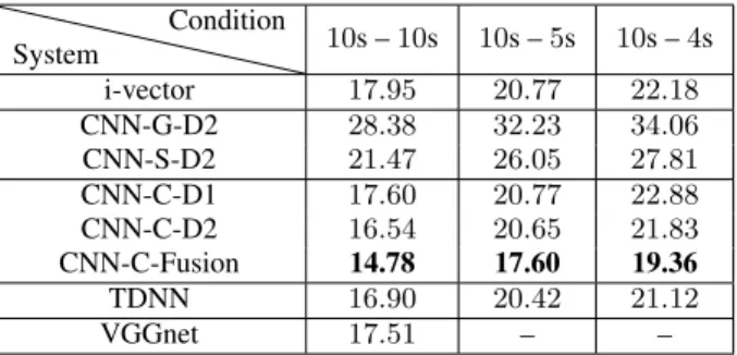
4.3. Results for the 10s enrolment condition
In this section, we evaluate performance for 10s enrolment con-ditions, described in Table 2. We do not show the performances of CNN-G-D1 and CNN-S-D1 for the sake of clarity, since their performance is inferior in each case to the -D2 system variants. From Table 2, we can see that when we aggregate fea-tures by average pooling, performance dramatically degrades compared to the i-vector system. This is consistent with [10]. The CNN-S-D2 system achieves a large 18%∼24% relative
im-1https://david-ryan-snyder.github.io/2017/10/
Table 2:EER (%) of SV in 10s-enrollment condition System Condition 10s –10s 10s –5s 10s –4s i-vector 17.95 20.77 22.18 CNN-G-D2 28.38 32.23 34.06 CNN-S-D2 21.47 26.05 27.81 CNN-C-D1 17.60 20.77 22.88 CNN-C-D2 16.54 20.65 21.83 CNN-C-Fusion 14.78 17.60 19.36 TDNN 16.90 20.42 21.12 VGGnet 17.51 – – provement over CNN-G-D2. Clearly, statistical pooling, which effectively incorporates variance information, enables an im-provement in performance. Compared with CNN-S-D2, the CNN-C-D2 system then obtains a further 22%, 20% and 21% relative improvements in 10s-10s, 10s-5s and 10s-4s evaluation respectively. In fact, CNN-C-D2 outperforms the i-vector sys-tem for each evaluation condition.
When we compare CNN-C-D2 with CNN-C-D1, the EER improves as expected; this demonstrates that dilation enlarges the receptive field to yield benefit for the SV task.
CNN-C-D2 obtains state-of-the-art performance in the 10s-10s evaluation, and achieves comparable performance to TDNN in the 10s-5s and 10s-4s evaluations as well. However when we fuse CNN-C-D1 and CNN-C-D2, termed CNN-C-Fusion, we obtain better performance for each evaluation. In fact CNN-C-Fusion system improves EER compared to the i-vector system by 17%, 15% and 12% in 10s-10s, 10s-5s and 10s-4s evalua-tions respectively.
Table 3:EER (%) of SV in 5s enrollment condition
System Condition 5s –10s 5s –5s 5s –4s i-vector 20.77 23.23 25.00 CNN-C-D1 20.07 25.35 25.75 CNN-C-D2 19.01 22.53 23.59 CNN-C-Fusion 17.60 20.42 21.83 TDNN 19.01 23.23 25.70 VGGnet – 23.16 –
4.4. Results for the 5s enrolment condition
In this section, we evaluate performance for 5s enrolment con-ditions, described in Table 3. We omit the performance of the CNN-G-D1/D2 and CNN-S-D1/D2 for the sake of clarity, since they are similar to 10s enrolment in Section 4.3.
Table 3 shows that the proposed CNN-C-D2 system obtains state-of-the-art performance in each evaluation. In Section 4.3, TDNN obtained similarly good performance in the 10s-5s and 10s-4s evaluation, however, for this shorter duration enrolment, TDNN is less robust. TDNN performance is slightly worser than the i-vector system in the 5s-4s evaluation, and CNN-C-D2 performs better than all tested systems for all experimental conditions.
VGGnet reported state-of-the-art performance in 5s-5s evaluation in [12], however the CNN-C-D2 system is shown to perform better for this evaluation.
When we then fuse the CNN-C-D1 and CNN-C-D2 sys-tems, termed CNN-C-Fusion, we gain 15%, 12% and 12%
rel-ative improvements for the 5s-10s, 5s-5s and 5s-4s evaluations respectively.
4.5. Discussion
C-D2 demonstrates consistent improvements over CNN-C-D1 since it has a larger receptive field. The dilated convo-lution enlarges the filter size by dilating the filter with zeros. However, it is possible that the two networks focus on differ-ent patterns. The filters enlarged by dilation tend to learn global features or patterns, while filters with no dilation are more prone to learn local features. We infer that the two networks are thus learning some information that may be complementary. This appears to be confirmed by the excellent performance achieved by the fusion system (termed CNN-C-Fusion).
We have compared the performance of average and statis-tical pooling. If we see from the Baum-Welch statistics point of view, average pooling can be viewed as 0th
-order statis-tics, whereas statistical pooling introduces variance which can be viewed as being2nd
-order statistics. The results conform that high-order statistics are significant for short-duration SV. However, it does not make full use of covariance, since it as-sumes that the covariance is diagonal. We thus proposed cross-convolutional-layer pooling to capture1st-order statistics for
modelling long-term speaker characteristics. Specifically, the activations of one convolutional layer are aggregated with the guidance of its successive layer. This technique achieved state-of-the-art performance in each evaluation condition. The results clearly demonstrate that cross-convolutional-layer pooling is a more efficient method for the aggregation of frame-level fea-tures.
5. Conclusions
In this paper, we present an improved deep embedding learn-ing method based on convolutional neural networks for short-duration speaker verification (SV). The dilated filters are de-signed to enable a tradeoff between computational efficiency and receptive-field size. The dilated convolution enables the network to learn long-term temporal content with relatively low computational complexity.
The proposed system aggregates frame-level features through cross-convolutional-layer pooling, which enables the system to exploit1st-order statistics. The proposed CNNs are
trained to discriminate variable-length input features between speakers in an end-to-end manner. After training, speaker em-beddings are extracted, and then similarity scores are calculated using a PLDA backend. On the modified female part of the NIST 2010 SRE evaluation, consisting of 10s and 5s enrolment conditions, the proposed approaches have achieved state-of-the-art performance in each evaluation condition. Specially, results show a 17% and 15% relative improvement for 10s-10s and 5s-5s evaluations respectively compared with the i-vector system. In future work, we aim to extend the proposed model to a larger number of speakers, to further investigate the data dependency of the feature learning approaches.
6. Acknowledgements
The authors would like to acknowledge the support of National Natural Science Foundation of China grant no U1613211.
7. References
[1] P. Kenny, G. Boulianne, and P. Dumouchel, “Eigenvoice modeling with sparse training data,”IEEE transactions on speech and audio processing, vol. 13, no. 3, pp. 345–354, 2005.
[2] D. Garcia-Romero and C. Y. Espy-Wilson, “Analysis of i-vector length normalization in speaker recognition systems,” inTwelfth Annual Conference of the International Speech Communication Association, 2011.
[3] P. Kenny, V. Gupta, T. Stafylakis, P. Ouellet, and J. Alam, “Deep neural networks for extracting Baum-Welch statistics for speaker recognition,” inProc. Odyssey, 2014, pp. 293–298.
[4] F. Richardson, D. Reynolds, and N. Dehak, “Deep neural network approaches to speaker and language recognition,”IEEE Signal Processing Letters, vol. 22, no. 10, pp. 1671–1675, 2015. [5] S. Ranjan and J. H. Hansen, “Improved gender independent
speaker recognition using convolutional neural network based bottleneck features,” Proc. Interspeech 2017, pp. 1009–1013, 2017.
[6] P. Kenny, “Bayesian speaker verification with heavy-tailed pri-ors.” inOdyssey, 2010, p. 14.
[7] N. Dehak, P. J. Kenny, R. Dehak, P. Dumouchel, and P. Ouellet, “Front-end factor analysis for speaker verification,”IEEE Trans-actions on Audio, Speech, and Language Processing, vol. 19, no. 4, pp. 788–798, 2011.
[8] C. Li, X. Ma, B. Jiang, X. Li, X. Zhang, X. Liu, Y. Cao, A. Kan-nan, and Z. Zhu, “Deep speaker: an end-to-end neural speaker embedding system,”arXiv preprint arXiv:1705.02304, 2017. [9] D. Snyder, D. Garcia-Romero, D. Povey, and S. Khudanpur,
“Deep neural network embeddings for text-independent speaker verification,”Proc. Interspeech 2017, pp. 999–1003, 2017. [10] E. Variani, X. Lei, E. McDermott, I. L. Moreno, and J.
Gonzalez-Dominguez, “Deep neural networks for small footprint text-dependent speaker verification,” inAcoustics, Speech and Signal Processing (ICASSP), 2014 IEEE International Conference on. IEEE, 2014, pp. 4052–4056.
[11] D. Snyder, P. Ghahremani, D. Povey, D. Garcia-Romero, Y. Carmiel, and S. Khudanpur, “Deep neural network-based speaker embeddings for end-to-end speaker verification,” in Spo-ken Language Technology Workshop (SLT), 2016 IEEE. IEEE, 2016, pp. 165–170.
[12] G. Bhattacharya, J. Alam, and P. Kenny, “Deep speaker embed-dings for short-duration speaker verification,” inProc. Interspeech 2017, 2017, pp. 1517–1521.
[13] A. Van Den Oord, S. Dieleman, H. Zen, K. Simonyan, O. Vinyals, A. Graves, N. Kalchbrenner, A. Senior, and K. Kavukcuoglu, “Wavenet: A generative model for raw audio,”arXiv preprint arXiv:1609.03499, 2016.
[14] V. Peddinti, D. Povey, and S. Khudanpur, “A time delay neural network architecture for efficient modeling of long temporal con-texts,” 2015.
[15] J. Ma, V. Sethu, E. Ambikairajah, and K. A. Lee, “Incorporating local acoustic variability information into short duration speaker verification,”Proc. Interspeech 2017, pp. 1502–1506, 2017. [16] M. Holschneider, R. Kronland-Martinet, J. Morlet, and
P. Tchamitchian, “A real-time algorithm for signal analysis with the help of the wavelet transform,” inWavelets. Springer, 1990, pp. 286–297.
[17] F. Yu and V. Koltun, “Multi-scale context aggregation by dilated convolutions,”arXiv preprint arXiv:1511.07122, 2015. [18] P. Wang, P. Chen, Y. Yuan, D. Liu, Z. Huang, X. Hou, and
G. Cottrell, “Understanding convolution for semantic segmenta-tion,”arXiv preprint arXiv:1702.08502, 2017.
[19] F. Yu, V. Koltun, and T. Funkhouser, “Dilated residual networks,” inComputer Vision and Pattern Recognition, vol. 1, 2017.
[20] L. Liu, C. Shen, and A. van den Hengel, “The treasure beneath convolutional layers: Cross-convolutional-layer pooling for im-age classification,” inProceedings of the IEEE Conference on Computer Vision and Pattern Recognition, 2015, pp. 4749–4757. [21] S. Ioffe and C. Szegedy, “Batch normalization: Accelerating deep network training by reducing internal covariate shift,” in Interna-tional conference on machine learning, 2015, pp. 448–456. [22] A. F. Martin and C. S. Greenberg, “The NIST 2010 speaker
recog-nition evaluation,” inEleventh Annual Conference of the Interna-tional Speech Communication Association, 2010.
[23] A. Paszke, S. Gross, S. Chintala, and G. Chanan, “Pytorch,” 2017. [24] D. Povey, A. Ghoshal, G. Boulianne, L. Burget, O. Glembek, N. Goel, M. Hannemann, P. Motlicek, Y. Qian, P. Schwarzet al., “The kaldi speech recognition toolkit,” inIEEE 2011 workshop on automatic speech recognition and understanding, no. EPFL-CONF-192584. IEEE Signal Processing Society, 2011.