Measuring Vulnerability to Poverty Using Long- Term Panel Data

SOEPpapers

on Multidisciplinary Panel Data Research

Measuring Vulnerability

to Poverty Using

Long-Term Panel Data

481

20

1

2

SOEPpapers on Multidisciplinary Panel Data Research

at DIW Berlin

This series presents research findings based either directly on data from the German

Socio-Economic Panel Study (SOEP) or using SOEP data as part of an internationally comparable

data set (e.g. CNEF, ECHP, LIS, LWS, CHER/PACO). SOEP is a truly multidisciplinary

household panel study covering a wide range of social and behavioral sciences: economics,

sociology, psychology, survey methodology, econometrics and applied statistics, educational

science, political science, public health, behavioral genetics, demography, geography, and

sport science.

The decision to publish a submission in SOEPpapers is made by a board of editors chosen

by the DIW Berlin to represent the wide range of disciplines covered by SOEP. There is no

external referee process and papers are either accepted or rejected without revision. Papers

appear in this series as works in progress and may also appear elsewhere. They often

represent preliminary studies and are circulated to encourage discussion. Citation of such a

paper should account for its provisional character. A revised version may be requested from

the author directly.

Any opinions expressed in this series are those of the author(s) and not those of DIW Berlin.

Research disseminated by DIW Berlin may include views on public policy issues, but the

institute itself takes no institutional policy positions.

The SOEPpapers are available at

http://www.diw.de/soeppapers

Editors:

Jürgen

Schupp

(Sociology, Vice Dean DIW Graduate Center)

Gert G.

Wagner

(Social Sciences)

Conchita

D’Ambrosio

(Public Economics)

Denis

Gerstorf

(Psychology, DIW Research Professor)

Elke

Holst

(Gender Studies)

Frauke

Kreuter

(Survey Methodology, DIW Research Professor)

Martin

Kroh

(Political Science and Survey Methodology)

Frieder R.

Lang

(Psychology, DIW Research Professor)

Henning

Lohmann

(Sociology, DIW Research Professor)

Jörg-Peter

Schräpler

(Survey Methodology, DIW Research Professor)

Thomas

Siedler

(Empirical Economics)

C. Katharina

Spieß

(Empirical Economics and Educational Science)

ISSN: 1864-6689 (online)

German Socio-Economic Panel Study (SOEP) DIW Berlin

Mohrenstrasse 58 10117 Berlin, Germany

Measuring Vulnerability to Poverty

Using Long-Term Panel Data

Katja Landau

Stephan Klasen

Walter Zucchini

Abstract

We investigate the accuracy of ex ante assessments of vulnerability to income poverty using cross-sectional data and panel data. We use long-term panel data from Germany and apply different regression models, based on household covariates and previous-year equivalence income, to classify a household as vulnerable or not. Pre-dictive performance is assessed using the Receiver Operating Characteristics (ROC), which takes account of false positive as well as true positive rates. Estimates based on cross-sectional data are much less accurate than those based on panel data, but for Germany, the accuracy of vulnerability predictions is limited even when panel data are used. In part this low accuracy is due to low poverty incidence and high mobility in and out of poverty.

Keywords: vulnerability, poverty, ROC, German panel data JEL classification: C23, C52, I32, O29

Acknowledgements: Funding from the Courant Research Centre: Poverty, Equity and Growth in support of this work is gratefully acknowledged. We would like to thank partic-ipants of the EUDN PhD Workshop 2011 in Amsterdam, the PEGNet Conference 2011 in Hamburg, and seminars in G¨ottingen and Dortmund for helpful comments and discussion.

∗_{Department of Economics, University of Goettingen}

†_{Corresponding author. Department of Economics, University of Goettingen; Courant Research Centre}

“[email protected]

1

Introduction

In order to reduce (income) poverty it is clearly relevant to be able to identify households that face the risk of falling into poverty in the future, i.e. to determine those that are vulnerable to poverty. Since the term “vulnerability” was brought under the spotlight by the World Development Report 2000/01 (World Bank, 2001) researchers have proposed different axiomatic approaches to concretize the concept, and have developed empirical approaches to estimate it. However, little attention has been paid to the accuracy of such estimates, or indeed to how accuracy might be appropriately defined in this context. The aim of the investigation described in this paper is to address these two issues.

Ideally, the assessment of vulnerability to poverty requires panel data, that is records of the same households over several years that can be used to capture information regarding the risks that households face (World Bank, 2001). Nevertheless approaches based on cross-sectional data have also been proposed (e.g. Chaudhuri (2002), Suryahadi and Sumatro (2003), G¨unther and Harttgen (2009), Jha and Dang (2010), Christiaensen and Subbarao (2005)). The reason for this is simply that panel data are relatively scarce, especially in developing countries where often only cross-sectional survey data are available.

Our investigation therefore covers methods for both cross-sectional and for panel data. The aim is to assess the potential accuracy of vulnerability predictions. Another goal is to identify components (covariates) that seem useful in the estimation of vulnerability to poverty.1

In our application, we focus on German households and use the German Socio-Economic Panel (SOEP) (specifically “Soepv26”) due to the fact that high-quality long-term panel data are available to predict and then validate vulnerability to poverty. The SOEP offers comprehensive coverage of household characteristics and income for 26 years and so we can observe, retrospectively, whether a household really did become poor. That enables us to compare the performance of different methods of estimating vulnerability (e.g. using panels of varying length) over several years.

Clearly a good estimate of vulnerability should identify a large proportion of those house-holds that will become poor, or will remain poor, in a specified future time interval, e.g. the following year, in the absence of intervention. However, that criterion can be met simply by

declaring all households to be vulnerable, since “even millionaires are vulnerable to poverty” (see e.g. Pritchett et al., 2000), but on its own, this criterion is not useful. A second criterion that needs therefore also to be taken into account is the estimate’s performance in identify-ing householdsthat will not become poor. The Receiver Operating Characteristic (ROC) is a well-established statistical instrument to quantify the performance of diagnostic methods; it takes account, not only of the proportion of households that are correctly identified as vulnerable (True Positive Rate, TPR) but also the proportion that are incorrectly declared to be vulnerable (False Positive Rate, FPR). The usual (scalar) criterion for assessing the accuracy of a diagnostic method from the ROC is the ”Area under the Curve” (AUC), which takes on values between 0 and 1. A method is regarded as more accurate than a competing method if its AUC is larger. A disadvantage of the AUC in our application is that it compares the performance of methods over theentire rangeof possible True Positive Rates. For the purpose of estimating vulnerability it is irrelevant whether one method is superior to another for small values of the TPR, such as TPR=10%; only large values of the TPR are of practical interest. In other words as a method-selection criterion, the AUC is insufficiently focussed in this application. The same applies to Selten’s measure of predictive success (Selten (1991), Selten and Krischker (1983)). One could restrict the range of TPRs considered by using a ”Partial ROC” (see, e.g. Thompson and Zucchini, 1989). Applying this idea, our approach is to compare the FPRs of different methods for aprescribedTPR. In the analyses that follows we use TPR=80% (sometimes 90%). A method will be regarded as being superior to a competing method if its FPR is smaller for the prescribed level of the TPR. We applied the ROC to compare the predictive performance of vulnerability es-timates based on methods that take account of household characteristics and previous-year equivalence income. We used rolling panels of different lengths to check the stability of the results retrospectively.

We find that methods that uses panel data are far superior in assessing vulnerability to poverty. We also find, however, that the predictive performance even with panel data is rather limited, i.e. one needs to declare many households to be vulnerable to capture most that will end up poor. We show that this is due to the relatively low overall poverty incidence as well as the high fluctuation in and out of poverty in Germany.

and give the definition that we use in our analysis. The regression models that were inves-tigated are defined. Some of these are suitable for cross-sectional data, and some for panel data. We give a detailed interpretation and discuss the assumptions made in the case of the former. Section 3 gives a brief account of the ROC and discusses its appropriateness in the context of vulnerability estimation. Section 4 describes the data and summarizes the results of our investigation. Section 5 concludes.

2

Vulnerability to poverty

2.1

Defining vulnerability to poverty

The term vulnerability has come into frequent use in the last two decades, especially in climate and poverty research (Dietz, 2006). The scientific use of the term evolved from two different concepts having their origin in disaster research in the eighties and nineties, namely “the Risk- or Natural-Hazard Approach” and the “Social Vulnerability Approach”. In the first approach vulnerability measures the intensity, or rather the severity, of external shocks on, e.g., a region (Dietz (2006), Yamin et al. (2005)). From this perspective vulnerability to poverty in a region might be explained by natural hazards, e.g. the occurrence and severity of earthquakes. A disadvantage of this approach is that data about such extreme events are rarely available, and their precise impact is difficult to assess. The second approach focuses on the micro level. Vulnerability is considered as a risk that exists due to the place of residence, as well as the structure and characteristics of households and individuals. Pioneering work is the “Entitlement Approach”, by Sen (1981) that is applied in the context of the “Social Vulnerability Approach” where levels and changes in entitlements measure the ability of households to withstand shocks such as droughts or rising food prices.

Current policy research in poverty reduction (see e.g. the World Development Report 2000/01) aims to alleviate vulnerability both to external shocks (financial crises, natural disasters, political turmoil, crime, etc.) and to household-specific shocks (unemployment, illness, changes in household structure, etc.). In the field of development economics the definition and interpretation of the term vulnerability would seem to be primarily based on remarks by Chambers (1989), as quoted by (Dietz, 2006). In his definition vulnerability has “two sides: an external side of risks, shock and stress to which a household or an

individual is subject; and an internal which is defencelessness, meaning a lack of means to cope without damaging loss”. Although closely related, poverty and vulnerability are two different concepts. The term poverty refers to a state at a (static) point in time usually measured ex post using household income or expenditure surveys, whereas vulnerability to poverty refers to a potential state in the future, i.e. an occurrence that may or may not occur in future. Therefore, unlike poverty, vulnerability has the nature of a probability forecast, an ex ante assessment of poverty risk. Assessing the accuracy of probability forecasts requires knowledge of the outcome, in our case whether or not the household really did become poor. Of course, one cannot expect perfect forecasts due to the stochastic nature of events affecting households. But a successful approach to measuring vulnerability to poverty would be able to identify households that are significantly more likely to be poor in a future period.

Since the publication of the World Development Report 2000/01 (World Bank, 2001) many researchers engaged in assessing vulnerability to poverty, mainly in developing coun-tries, in terms of the definition of that report. In it vulnerability is defined as “the risk that a household or individual will experience an episode of income or health poverty over time. But vulnerability also means the probability of being exposed to a number of other risks (violence, crime natural disasters, being pulled out of school”) (World Bank, 2001). In view of its dynamic structure, the assessment of vulnerability to poverty requires panel data (World Bank, 2001). Nevertheless, many authors have based their analysis on cross-sectional data (e.g. Chaudhuri (2002), Christiaensen and Subbarao (2005), G¨unther and Harttgen (2009), Jha and Dang (2010) ), mainly because panel data are rarely available in developing countries.

Although much attention has been paid to defining and assessing vulnerability to poverty there is currently no unique generally accepted definition of vulnerability based, e.g. on some economic theory, and therefore no accepted indicators and methods for its measurement (Chambers,1989). Concepts for vulnerability to poverty that have been developed include Vulnerability as Exposure to Risk (VER), Vulnerability as Expected Poverty (VEP) e.g. Chaudhuri (2002), Pritchett et al.(2000), Vulnerability as Low Expected Utility (VEU) e.g. Ligon and Schechter (2003) and an Axiomatic Approach that combines expected poverty with expected poverty depth, e.g. Calvo and Dercon (2005).

of VEP (Hoddinott and Quisumbing (2003), Chaudhuri(2002)). In the simplest case vul-nerability is just the probability that an individual or household will fall below a predefined (absolute or relative) poverty line in the future. As measure of well-being in our investiga-tion we use the yearly equivalence-income, i.e. the sum of net income and imputed rent (see, e.g., Frick and Krell, 2009) weighted by modified OECD equivalence scales. In what follows we will refer to this briefly as “income”. When referring to vulnerability it is necessary to specify the time horizon under consideration for which the household is vulnerable; this is often taken as one year (e.g. Chaudhuri et al. (2002), G¨unther and Harttgen(2009), Jha and Dang (2010)). We too focus on the one-year horizon, but also briefly consider multi-year cases.

In the framework of VEP, and for a n–year horizon, household his defined to be vul-nerable if the probability that the household income will fall below the poverty line in at least oneof the subsequentn-years exceeds some pre-specified cutoff. If the income shocks in each year are assumed to be independent, this probability is given by

v_n(h) = 1 − Pr(y_t(₊₁h) > z) Pr(y_t(₊₂h) > z)· · ·Pr(y_t(₊h)_n> z) (1)

wherey(_th)is the current income of householdhandzthe predefined poverty line. The cutoff probability is usually set at 0.5, or alternatively at the estimated current poverty rate. (For details, see Chaudhuri et al. (2002)). Of course these specifications are arbitrary.

2.2

Estimating vulnerability to poverty

In principle, two empirical approaches to determine this probability could be pursued. First, one could actually try to specify for each household future states of the world, determine their likelihood and the income attached to them and calculate vulnerability to poverty in this way. This is, for example, done in Povel (2009) which uses information on perceived probabilities of future shocks and their severity as stated by households. While this is an interesting approach, it makes strong assumptions about the ability of households to judge risks and their impact accurately and it assumes independence of risks. A second approach, more common in the literature, has been to determine vulnerability to poverty by predicting

incomes based on covariates. In this approach the probability vn(h) is usually estimated

using regression models (e.g. Chaudhuri et al. (2002), Christiaensen and Subbarao (2005)) in which covariates Xt(h) are mainly household characteristics, but also macro or climate

variables (e.g. Christiaensen and Subbarao (2005)) or, possibly, income or consumption in previous years. If panel data are available then it is possible to capture some of the dynamic structure of vulnerability. However, if the model for income is of the form

y_t(h)=X_t(h)β+e(_th) (2)

then, in order to estimate vn(h), it is first necessary to forecast the future values of the

covariates. Here the e(_th) represent the residuals in the model, interpreted as positive or negative “shocks”, or deviations from the expected income. In the case where only cross-sectional data are available, several additional and stringent assumptions are needed to estimate vulnerability. In particular we need to assume that vulnerability remains constant over time, that neither the household covariates nor the expected income change over time. Only the residuals (shocks) change. In effect this model assumes that the inter-temporal variance can be measured using the cross-sectional variance, and that shocks are serially uncorrelated.

We investigate six models for predicting incomes that are then used to estimate vul-nerability to poverty. Note that we do not specify ’causal’ models of an income-generation process, but correlation-based models whose aim is limited to that of estimating (predict-ing) the future income of households. The models differ in the type of data available: cross-sectional data (P1-P3) or panel data (P4-P6), and the covariates available: household covariates only (P1 and P2); income only P3 or both household covariates and income (P4 - P6). Some of the models are based on current year household covariates (P2, P4, P5), and some on those of the previous year (P1, P6), as data for the current year are often not available. The models P4 and P5 differ in the regression coefficient ˆγof the income covari-ate; in P5 ˆγ is set to one, so that the household covariates explain thechange in incomein successive years.

ˆ y(_th)=X_t−(h)₁βˆ (P1) ˆ y(_th)=X_t(h)βˆ (P2) ˆ y(_th)=y(_t−h)₁ (P3) ˆ y_t(h)=X_t(h)βˆ+y_t−(h)₁ˆγ (P4) ˆ yt=X_t(h)βˆ+y_t−(h)₁ (P5) ˆ yt=X_t−(h)₁βˆ+y_t−(h)₁ˆγ (P6)

where X_t(h) represents the covariates of household h at time t; β and γ are regression coefficients ande(th) is the residual for householdhat timet.

A household will be declared vulnerable under a given model if the estimate ˆytis below a predetermined cutoff, which can be different for each model. To apply these models (except P3) one needs first to determine which of the available covariates are best suited for predicting income. This variable selection issue is discussed in 4.5. We now consider the problem of comparing the accuracy of the above six models for the purpose of estimating vulnerability.

Readers will readily note that this empirical approach has some resemblence to the macro literature on the consumption function and the predictability of consumption (e.g. Hall, 1978; Hall and Mishkin, 1982; Lusardi, 1996). That literature investigated whether consumption change was predictable (and closely related to income change), or followed a random walk. Some of that literature also investigated the predictability of income (e.g. Lusardi, 1996) but did not specifically consider the accuracy of the predictions, our approach to test the accuracy of predictions could also be applied to that literature.

3

Assessing the accuracy of vulnerability estimates

In the literature on vulnerability relatively little attention has been paid to the question of the accuracy of vulnerability estimates. Exceptions include Ligon and Schechter (2004), Jha and Dang (2010) and Zhang and Wan (2009).

Ligon and Schechter (2004) conduct Monte Carlo experiments on artificially generated databases (in which future welfare is known) under different circumstances (stationary, non-stationary environment, presence or absence of measurement error). They assess the accu-racy of vulnerability using the Mean Squared Error (MSE) and the Spearman Rank Corre-lation, as a function of the panel size and the number of panel waves. However, they base their conclusions on simulated data which, as they point out “of course assume away much of the real world data”. Their analysis on the Vietnamese Household Survey (2 periods) and the Bulgarian Household Budget Survey (12 periods) compare the relationships between different vulnerability measures, e.g. the correlation between them. The estimator that was identified as best in their experiments was applied to the surveys and the determined vul-nerability measure was decomposed into measures of poverty, aggregated and idiosyncratic risk, as well as measurement error. But the decomposition does not study the accuracy of estimated vulnerability, i.e. which households became poor and which did not.

Jha and Dang (2010) measure the accuracy as the proportion of households in the sample that were correctly classified. On this basis they find that the vulnerability estimates ’do a reasonably good job’. However, the proportion of correct classifications can be a mislead-ing measure of the quality of a diagnostic method, because it is strongly affected by the proportion of poor and non-poor households in the population. The Receiver Operating Characteristics (ROC), discussed below, was specifically designed to overcome this problem. Zhang and Wan (2009) analyse the impact of different income measures, poverty and vulnerability lines on the accuracy of vulnerability estimates. They define accuracy as the following fraction: the number of households correctly declared vulnerable divided by the total number of households that were declared vulnerable. This measure fails to take into account the households which become poor but were classified as non-vulnerable. Again, the ROC overcomes this problem.

tech-nique, and hence for comparing the performance of different techniques. It is applied in many fields. (See, e.g. Egan (1975), Spackman (1989), Thompson and Zucchini (1989), Swets et al. (2000), Fawcett (2003).) In medical contexts it is used to quantify the trade-off between the sensitivity or True Positive Rate (TPR, i.e. the probability to correctly diagnose a diseased patient) and the “specificity” (the probability to correctly diagnose a non-diseased patient); the latter is equal one minus the “false alarm” rate, i.e. one minus the False Positive Rate (FPR). In our case we wish to assess how well different methods are able to diagnose future poverty, i.e. how accurately they predict which households will become poor and which will not.

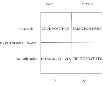
The diagnosis proceeds by first fitting the model to be used to estimate the future income of each household. Then a cutoff (the vulnerability line) is specified such that households whose forecasted income fall below the cutoff are classified as vulnerable; the others are classified as non-vulnerable. Thus four different diagnosis-outcome combinations are possible, as shown in the “confusion matrix” in Figure 1.

TRUE CLASS

poor non-poor

HYPOTHESZED CLASS vulnerable

non vulnerable

TRUE POSITIVES FALSE POSITIVES

FALSE NEGATIVES TRUE NEGATIVES

P

N

Figure 1: Confusion matrix

By varying the cut-off point we can balance the rates at which the two types of error (false negatives and false positives) occur. The ROC is simply a graph in which the False Positive Rate (FPR) is plotted on the x-axis against the True Positive Rate (TPR) on the y-axis. The ROC is a non-decreasing function that starts at the point (0,0) and ends at the point (1,1). Roughly speaking, the faster the curve approaches the level y=1 the better the

diagnostic method; the method is perfect if its ROC reaches y=1 straight away, i.e. it passes through the point (0,1). The ROC enables us to compare the diagnostic performance of the six different models listed above over the entire range of possible cutoffs that could be used to decide whether or not a household is to be declared vulnerable. The cutoffs for different models need not be the same.

The ROC enables us to determine the cost, measured in terms of the FPR, that is needed to achieve prescribed TPR. Suppose, for example, that we wish to identify at least 80% of all households that will be poor in the coming year. The value TPR=0.8 determines retrospectively the vulnerability to poverty line (VPL) which in turn determines the FPR. If the resulting FPR is high (e.g. 40%) then the absolute number of “false alarms” might well be too large for this method of specifying vulnerability to be of practical use.

4

Analysing vulnerability estimates using SOEP data

4.1

Data structure and organization

The Socio-Economic Panel (SOEP) is a panel study of German households, started in 1984, and carried out by the German Institute for Economic Research (DIW), Berlin. For our survey we used the version “Soepv26”. As units of observation we chose private households so as to make the results comparable to the cited vulnerability studies that are all based on households. We focus on harmonised variables based on the Cross-National Equivalent File (CNEF) due to their reliability and their practical application. The covariates in the regression models included variables that are aggregated at the household level as well as characteristics of the household head. To obtain representative results for the population (of households) the sample sizes were weighted using the supplied household-level cross-sectional weights and staying probabilities.

The information extracted at the household level includes net income and imputed rent, age structure, size of residence and variables that relate to the employment situation of the household members, namely the total working hours (in the previous year) and the number of full-time and part-time employees. The covariates chosen relating to the household head include sex, marital status, education, employment sector (or if not employed the information that the head is unemployed) and state of ownership of residence.

Specially care is needed to take account of the different timing structure of income (retro-spective) (see e.g. Frick et al. (2008), Frick and Krell (2009)) and household characteristics (perspective, except for the number of working hours). The income that is recorded un-der the survey year in fact refers to the income in the previous year, but allocated by the household members in the survey year. Consequently the following two adjustments were made: The income for yearthad to be extracted from the records of yeart+ 1. The second adjustment is necessitated by the fact that household composition can change from year to year and, if it does, this affects the components of the resulting equivalence income, which we computed using modified OECD equivalence scales (see, e.g., Statistisches Bundesamt, 2008). In contrast to most surveys we use the household composition in the year in which the income accrued, and not that from the survey year. This introduces some bias if indi-viduals, who accrued income in the previous year, have joined or left the household (Debels and Vandecasteele, 2008).2 _{We adjusted the equivalence income for inflation using 2005 as}

basis year.

When assessing models based on panel data, we would normally require two waves to estimate vulnerability and a third wave to compute the ROC, and thereby quantify the accuracy of the estimate. However, the one-year delay for the income information to become available leads to our needing one more SOEP wave than would be necessary if income information were available at the end of the relevant year. We therefore base our analysis on balancedfour-year-panels over the years 1992 to 2009. Although the database covers earlier years, income data for Eastern Germany are only available from 1991 (we start one year later with our analysis). We usedbalancedfour-year panels, that is we removed households which were not represented in all four years.

Although the SOEP is a relatively complete panel study, there are some missing data due to (item)- non-response or flaws such as implausible responses by individuals or entire households. For our purposes this problem occurs mainly for categorial variables; missing income values and continuous variables have been imputed (see e.g. Frick and Grabka (2004) and (2007)). Two situations were of concern: missing information for the household head

2_{If one chose to consider the current year household composition, a similar and arguably more problematic}

(e.g. education, industry sector) and biased variables (due to individual missing values, e.g. a year of birth is not available, or a value was imputed). For the first case we excluded the household from the four-year panel even if the information is missing in just one year. Between 6 and 16% of households were excluded. In the second case we used the (possibly biased) information that is available.

We also investigated the alternative of excluding households only in those years in which information was missing. A disadvantage of doing that is that predictions based on models P1-P6 refer to (slightly) different sets of households and consequently, strictly speaking, the resulting ROCs are not directly comparable. These two procedures led to very similar regression estimates and so we only report those based on the first method.3

We note that the estimates of vulnerability in our analysis apply to the survey year and not to the following year. That is because the income of households becomes available in the year that follows the survey year. In other words we estimate vulnerability for the present, not for the future. This problem occurs in all surveys in which past income is solicited. There is, however, the advantage that most of the current values of the covariates might already be available to the researcher or policy-maker in the relevant year; they do not have to be forecasted.

4.2

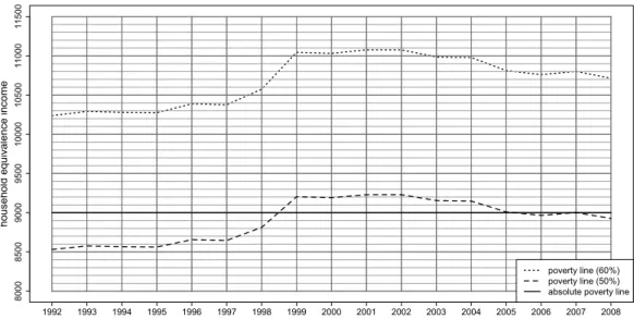
Household-based poverty lines in Germany 1992-2008

In order to classify a household as poor or non-poor we must specify a poverty line. The literature on poverty research distinguishes between absolute and relative poverty lines, where the former is a fixed amount and the latter is determined from the income distribution of the population. In Germany it is common practice to use a relative poverty line, set at either 50% or 60% of the median per capita income (see e.g. Stauder and H¨uning (2004)). The latter are displayed in Figure 2 for the period 1992 to 2008, where time-axes represents the “year of occurence”, and not the survey year. (As explained above, income information

3_{However, if more data are missing then the results could differ substantially. Missing household covariates}

are especially problematic if one only using household covariates for predicting income. Such missing values are less problematic if the previous year income is used in the regression. As we will show, previous income is the strongest predictor of present income.

is only available in the year following the survey.) As our observation units are households the median equivalence income is determined on the basis of households, i.e. one entry per household (Stauder and H¨uning, 2004), where (equivalence) income is determined using the modified OECD household equivalence scales. The 50% poverty line rose quite sharply in 1999, it remained approximately constant until 2004 and then decreased slightly after that. For a discussion of the determinants of these changes see Maiterth and M¨uller, (2009).

In order to estimate vulnerability it is necessary to specify the value of the poverty line in the next period. In the case of relative poverty definition the future value of the poverty line is unknown and so has to be estimated, for example by its current value. To avoid the additional source of variation that arises when forecasting the poverty line, we used an absolute real poverty line in our analysis, namely 9 000e, a value that is reasonably close to the (50% of median) relative poverty line.

1992 1993 1994 1995 1996 1997 1998 1999 2000 2001 2002 2003 2004 2005 2006 2007 2008 8000 8500 9000 9500 10000 10500 11000 11500

household equivalence income

poverty line (60%)

poverty line (50%) absolute poverty line

Figure 2: Relative and absolute poverty lines 1992 to 2008

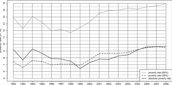
Figure 3 displays the percentage of poor households corresponding to the three poverty lines in Figure 2. The poverty rate corresponding to the absolute poverty line is higher than that for the 50% relative poverty line up to 1998 and then lower until 2006.

1992 1993 1994 1995 1996 1997 1998 1999 2000 2001 2002 2003 2004 2005 2006 2007 2008 5 6 7 8 9 10 11 12 13 14 15 16

poverty rate (in %)

poverty rate (60%) poverty rate (50%) absolute poverty rate

Figure 3: Relative and absolute poverty rates 1992 to 2008

Although “even millionaires are vulnerable to poverty” (see e.g. Pritchett et al.(2000)), we have assumed that few households whose real annual income per adult equivalent exceeds 30 000eare at risk of becoming poor in the immediate future. (In all our samples, comprising between 6 000 and 10 000 households, only between 0 and 10 such households were observed.) The reason for excluding wealthier households is to focus the regression models on the (lower) income range that is of interest here by removing potentially influential observations that are not pertinent to the objective of estimating vulnerability to poverty. We therefore restricted our balanced four-year panel to those households whose per equivalent income is less than 30 000ein each of the four years.

4.3

Descriptive statistics of the poor over time

The probability that households move into or out of poverty over time is obviously relevant for assessment of vulnerability. In situations where the poor stay in poverty, and the non-poor seldom become non-poor, the terms non-poor and vulnerable are effectively synonymous. This is not the case if a substantial proportion of households frequently change between being poor and non-poor. We give some descriptive statistics relating to this issue for our data.

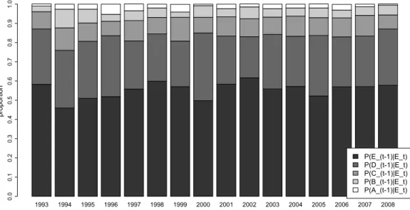
[12 000,18 000), [18 000,22 000), [22 000,30 000); we denote them by E, D, C, B, A. Note that E represents the group that we have defined as poor.

Figure 4 shows the proportion of thecurrently poor decomposed by income categories in theprevious year. Thus, e.g., 58% of the poor in 1993 were poor in 1992, 29% of the poor in 1993 were in group D 1992, 9% were in group C, 3% in B and 1% in A. The decompositions vary over the 16-year-horizon investigated, but not dramatically. They confirm that there is indeed a strong persistence in poverty but that a substantial proportion (around 40%) of poor households were not poor in the previous year.

1993 1994 1995 1996 1997 1998 1999 2000 2001 2002 2003 2004 2005 2006 2007 2008 0.0 0.1 0.2 0.3 0.4 0.5 0.6 0.7 0.8 0.9 1.0 proportion P(E_(t-1)|E_t) P(D_(t-1)|E_t) P(C_(t-1)|E_t) P(B_(t-1)|E_t) P(A_(t-1)|E_t)

Figure 4: Thecurrently poor decomposed by income categories in the previous year

For later explanations, it is also relevant to consider the distribution ofprevious income status forcurrently non-poor households, denoted byN Pt. Figure 5 shows that of the non-poor in 1993 about 5% had been non-poor in 1992, 15% had come from group D, 40% from group C, 22% from B and 18% from A.

1993 1994 1995 1996 1997 1998 1999 2000 2001 2002 2003 2004 2005 2006 2007 2008 0.0 0.1 0.2 0.3 0.4 0.5 0.6 0.7 0.8 0.9 1.0 proportion P(E_(t-1)|NP_t) P(D_(t-1)|NP_t) P(C_(t-1)|NP_t) P(B_(t-1)|NP_t) P(A_(t-1)|NP_t) 0.0 0.1 0.2 0.3 0.4 0.5 0.6 0.7 0.8 0.9 1.0

Figure 5: Distribution ofprevious income status forcurrently non-poor households

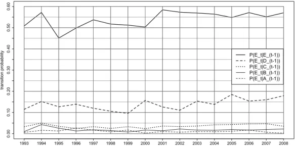
Figure 6 shows the more conventional transition proportions from each of the five income groups in yeart−1 to poverty in yeart. Note that these have a different interpretation to the proportions shown in Figure 3 and that, among other things, these transition proportions need not sum to one, whereas those in Figure 3 do. Summarizing the Figure as a whole: between 45% and 60% of poor households remained poor (in the following year), 10–20% from group D became poor, and less than 5% of households in each of groups C, B and A became poor.

0.00 0.10 0.20 0.30 0.40 0.50 0.60 1993 1994 1995 1996 1997 1998 1999 2000 2001 2002 2003 2004 2005 2006 2007 2008 transition probability P(E_t|E_(t-1)) P(E_t|D_(t-1)) P(E_t|C_(t-1)) P(E_t|B_(t-1)) P(E_t|A_(t-1))

Figure 6: Transition probability of the poor over time

In general we can conclude that although poverty has exhibited strong temporal persis-tence, a substantial proportion of the poor were in one of the non-poor income groups in the previous year. Secondly 40-55% of poor households manage to escape poverty in the following year. Given this high level of mobility in and out of poverty (including from higher levels of incomes), it is clear that we cannot expect a perfect prediction of those vulnerable to poverty.

4.4

Methods

The empirical analysis outlined here was performed using rolling balanced 4-year- panels between 1992 and 2009. We first identified which of the available household variables can be shown to improve the prediction of household income. Tables of typical results are presented in the next section. The information available for the first two years of each panel was used to forecast the income of each household in the third year using each of the models P4 - P6. For models P1 - P3 (which are based on cross-sectional data) only the information from the second year of the panel was used to forecast the income in the third year. For the models P2, P4 and P5 it was assumed that household information (but not the income) was also available for the third year and could be also be used for forecasting the income in that year.

The observed incomes in the third year were then used to determine which households were poor in that year and which were not. The reason why we needed a four-year panel is that the income for the third year is only published in the following year, i.e. in the fourth year. To construct the ROC (a plot of the FPR against the TPR) we simply counted the total number of true positives and the number of false positives in the third year for each possible cutoff (vulnerability line) applied to the predicted income for the third year. As the vulnerability line is increased so both the TPR and FPR also increase.

For the purposes of illustration we focus on the vulnerability line that leads to TPR = 80%, i.e. the vulnerability line is selected so that 80% of the households that are poor in the third year of the panel would have been classified as vulnerable at the end of the second year. (We also consider the case TPR=90%.) Despite the fact that all the models P1 - P6 are estimating the same thing (household income in year 3) the vulnerability lines that lead to TPR=80% can differ from model to model. Consequently the corresponding FPRs differ and, as is shown below, the differences can be substantial. Clearly, for a specified TPR, the model with the smallest FPR is the best, because it identifies the specified proportion of households that are poor in year 3 but leads to the smallest number of false alarms (i.e. households that were classified as vulnerable but did not become poor in year 3).

The above computations were carried out to determine the ROC for each of the six models and for each year in the period 1994 to 2008 and hence, for each model and each of these years:

• the vulnerability lines that lead to TPR=80% and to TPR=90%,

• the relationship between the vulnerability line and the proportion of vulnerable house-holds,

• the FPR associated with TPR=80% and with TPR=90%,

The above refers to the estimation of one-year-ahead vulnerability. We also investigated the accuracy of n-year-ahead vulnerability forn= 2,3,4. Thus, for example, the two-year case is that in which a household was (retrospectively) defined as poor if it was poor in

at least one of the two years subsequent to the vulnerability forecast. Clearly, a longer panel was needed to assess the accuracy of the multi-period vulnerability estimates. As is

to be expected, different horizonsnlead to different ROCs and the accuracy decreases asn

increases.

4.5

Results

In order to apply models in Section 2.2, apart from P3, we first determined which of the avail-able household covariates are useful in predicting household income. These are listed in Tavail-able 1. Several additional covariates were investigated, e.g. employment in the public/private sector, but are not included in the regression because they led either to multicollinearity or their inclusion did not lead to a significant improvement. Here we will give, as an example, details of the forecasts for the year t = 1996 and for the models P1, P4 and P6 which we will label P196,P496and P696, respectively.4

Estimateβ using y(₉₅h)=X₉₅(h)β+e(₉₅h)

Forecast using yˆ₉₆(h)=X₉₅(h)βˆ

(P196)

Estimateβ andγ using y₉₅(h)=γy₉₄(h)+X₉₅(h)β+e(₉₅h)

Forecast using yˆ(₉₆h)= ˆγy₉₅(h)+X₉₆(h)βˆ

(P496)

4 _{A number of different alternatives distributions were fitted to the residuals in the regression models.}

As income is often assumed to be approximately lognormally distributed many authors use the logarithm of income as response variable in the regression. However, with our data that transformation leads to residuals that are obviously not normally distributed; their distribution is skewed, and the kurtosis is not equal to 3. This can be explained by the fact that we only consider households whose annual income is less than 30 000e. As already mentioned, we excluded wealthier households from our analysis in order to remove potentially influential observations that are not relevant to the objective of estimating vulnerability to poverty. In our survey we used homoskedastic regression models in contrast to other surveys (see e.g. Chaudhuri et al. (2002)). We did experiment with various heteroskedastic regression models in which the variance is expressed as a function of the some the covariates, but the improvement in the fit was negligible.

Estimateβ andγ using y₉₅(h)=γy₉₄(h)+X₉₄(h)β+e(₉₅h)

Forecast using yˆ(₉₆h)= ˆγy₉₅(h)+X₉₅(h)βˆ

(P696)

variables description

income equivalence income of the household in the previous year

sex sex of household head

(male, female)

n[0,18) number of individuals aged below 18

n[18,34) number of individuals aged at least 18 and below 34

n[34,59) number of individuals aged at least 34 and below 59

n[59-) number of individuals above 59

family status family status of the household head

(5 levels: married; single; widowed; divorced; separated)

working hours sum of working hours of all household members in the previous year

industry employment sector of the household head

(10 levels: not employed; agriculture; energy; mining; manufac-turing; construction; trade; transport; bank, insurance; services)

owner owner status of residence (3 levels: owner; main-tenant;

sub-tenant) size of residence

size of residence2

size of residence in square meters quadratic term

education highest level of education of the household head

(5 levels: secondary school; intermediate school; a-level or tech-nical degree; other degree; no school degree)

n(full-time work) n(full-time work)2

number of household members in full-time employment quadratic term

n(part-time work) number of household members in part-time employment

Table 1: Description of the variables used in the regression. The baseline levels for the categorical variables are indicated in boldface.

Estimate Std. Error t value Pr(>|t|) (Intercept) 18860.31 494.09 38.17 <0.001 *** sex: female -645.31 185.86 -3.47 <0.001 *** n[0,18) -1603.88 103.94 -15.43 <0.001 *** n[18,34) -1477.45 174.63 -8.46 <0.001 *** n[34,59) -1139.13 187.16 -6.09 <0.001 *** n[59−) -216.37 213.65 -1.01 0.311

family status single -89.85 289.37 -0.31 0.756

family status widowed 298.52 284.71 1.05 0.294

family status divorced -1137.05 286.36 -3.97 <0.001 ***

family status separated -982.72 620.49 -1.58 0.113

working hours in previous year 0.19 0.10 1.92 0.055 .

industry: agriculture -1036.88 751.73 -1.38 0.168 industry: energy 3324.15 843.63 3.94 <0.001*** industry: mining 814.35 1431.17 0.57 0.569 industry: manufacturing 1200.30 331.92 3.62 <0.001 *** industry: construction 1032.68 362.76 2.85 0.004 ** industry: trade 85.65 361.66 0.24 0.813 industry: transport 1524.63 474.78 3.21 0.001 ** industry: bank,insurance 3855.56 641.36 6.01 <0.001 *** industry: services 1044.26 310.57 3.36 <0.001 ***

owner: main tenant -933.66 183.48 -5.09 <0.001 ***

owner: sub tenant -1433.11 416.23 -3.44 <0.001 ***

size of residence 68305.67 6201.06 11.02 <0.001 ***

(size of residence)2 _{-22455.11 4773.50 -4.70 <0.001 ***}

education: intermediate school 1014.66 185.81 5.46 <0.001 ***

education: a-lev./tech. degree 2017.96 226.69 8.90 <0.001 ***

education: other degree -1535.13 474.83 -3.23 0.001 **

education: no school degree -1841.39 560.70 -3.28 0.001 **

n(full-time work) 145517.55 12793.75 11.37 <0.001 ***

n(full-time work)2 _{-37514.93 6852.48 -5.47 <0.001 ***}

n(part-time work) 1145.58 260.20 4.40 <0.001 ***

adjusted R-squared 0.294

no. observations (unweighted) 4493

F-statistic 61.15 (df: 30,4301)5

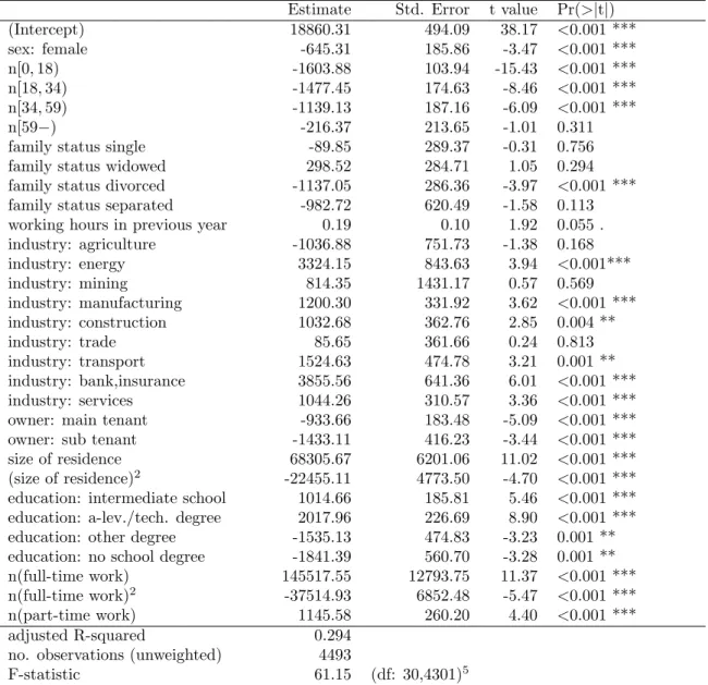
Table 2: Regression results Model P196

Estimate Std. Error t value Pr(>|t|)

(Intercept) 9037.08 449.21 20.12 <0.001 ***

income previous year 0.59 0.01 47.78 <0.001 ***

sex: female -98.63 150.67 -0.65 0.513

n[0,18) -608.48 86.57 -7.03 <0.001 ***

n[18,34) -713.33 142.06 -5.02 <0.001 ***

n[34,59) -608.74 151.70 -4.01 <0.001 ***

n[59−) -441.87 172.76 -2.56 0.011 *

family status: single 263.21 234.03 1.12 0.261

family status: widowed 287.59 230.14 1.25 0.212

family status: divorced -438.70 231.94 -1.89 0.059 .

family status: separated -776.46 501.58 -1.55 0.122

total working hours of previous year -0.37 0.08 -4.54 <0.001 ***

industry: agriculture -28.93 608.02 -0.05 0.962 industry: energy 1995.84 682.50 2.92 0.003 ** industry: mining -89.94 1157.02 -0.08 0.938 industry: manufacturing 454.61 268.75 1.69 0.091 . industry: construction 732.07 293.30 2.50 0.013 * industry: trade 264.75 292.36 0.91 0.365 industry: transport 789.27 384.09 2.05 0.040 * industry: bank,insurance 1764.89 520.27 3.39 <0.001 *** industry: services 354.80 251.46 1.41 0.158

owner: main tenant -640.40 148.44 -4.31 <0.001 ***

owner: sub tenant -1072.11 336.53 -3.19 0.001 **

size of residence 31493.88 5071.40 6.21 <0.001 ***

(size of residence)2 _{-8476.78 3869.65 -2.19 0.029 *}

education: intermediate school 334.75 150.87 2.22 0.027 *

education: a-level/technical degree 676.58 185.38 3.65 <0.001 ***

education: other degree -606.28 384.31 -1.58 0.115

education: no school degree -761.70 453.80 -1.68 0.093 ,

n(full-time work) 102425.57 10380.87 9.87 <0.001 ***

n(full-time work)2 _{-10615.55 5567.63 -1.91 0.057 .}

n(part-time work) 945.36 210.37 4.49 <0.001 ***

adjusted R-squared 0.539

no. observations (unweighted) 4493

F-statistic 164.2 (df: 31,4300)

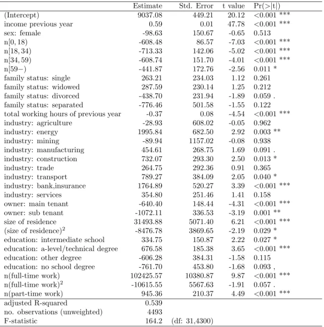
Table 3: Regression results Model P496, which uses concurrent values of the household

Estimate Std. Error t value Pr(>|t|)

(Intercept) 6167.68 466.17 13.23 <0.001 ***

income previous year 0.61 0.01 47.65 <0.001 ***

sex: female -23.98 154.07 -0.16 0.876

n[0,18) -311.02 88.74 -3.50 <0.001 ***

n[18,34) -125.59 140.67 -0.89 0.372

n[34,59) 1.32 150.25 0.01 0.993

n[59−) 218.94 172.50 1.27 0.204

family status: single 873.94 235.33 3.71 <0.001 ***

family status: widowed 325.65 235.60 1.38 0.167

family status: divorced -172.52 239.76 -0.72 0.472

family status: separated 768.38 454.72 1.69 0.091 .

Working hours total of household 0.15 0.08 1.86 0.063 .

industry: agriculture -541.30 635.59 -0.85 0.394 industry: energy 1693.47 638.70 2.65 0.008 ** industry: mining 95.04 986.31 0.10 0.923 industry: manufacturing 544.80 274.63 1.98 0.047 * industry: construction 441.78 298.92 1.48 0.140 industry: trade 252.16 299.53 0.84 0.400 industry: transport 633.47 405.16 1.56 0.118 industry: bank,insurance 1601.72 518.89 3.09 0.002 ** industry: services 278.05 261.43 1.06 0.288

owner: main tenant -620.23 152.85 -4.06 <0.001 ***

owner: sub tenant -1437.91 339.71 -4.23 <0.001 ***

size of residence 23364.76 5184.32 4.51 <0.001 ***

(size of residence)2 _{-5758.70 4013.95 -1.43 0.151}

education: intermediate school 256.92 153.55 1.67 0.094 .

education: a-level/technical degree 701.04 190.56 3.68 <0.001 ***

education: other degree -698.80 389.88 -1.79 0.073 .

education: no school degree -749.81 461.76 -1.62 0.104

n(full-time work) 17258.20 10605.28 1.63 0.104

n(full-time work)2 _{-11713.60 6134.41 -1.91 0.056 .}

n(part-time work) 158.85 218.85 0.73 0.468

adjusted R-squared 0.520

no. observations (unweighted) 4493

F-statistic 152.6 (df: 31,4300)

Table 4: Regression results Model P696 (with previous-year household covariates)

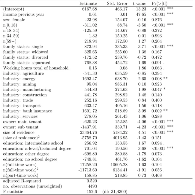
The estimated regression coefficients have the expected signs. Model P496 and Model

P696 have substantially higher coefficients of determination than Model P196, not only for

1995, but for all the years investigated. That gives a clear indication that a household’s (equivalence) income in a given year is an important covariate for predicting its income in the following subsequent year, i.e. that predictions based only on household cross-sectional data are much less accurate than those based on panel data. The ROC analysis that follows

will quantify this difference in more practical terms.

Model P496 and P696 produce similar results, see Tables 3 and 4. A possibility for

this is that most characteristics change little from year to year if the household head does not change. Secondly, it would seem that, for the population of lower-income households investigated here, the available covariates have little explanatory power once previous income has been taken into account.

The results of our analysis of the six models P1 - P6 regarding their relative accuracy in predicting household income can be summarized as follows: Regarding the models based on cross-sectional data, Model P2, which uses actual household characteristics, provides slightly more accurate predictions than Model P1, which is based on previous-year household characteristics. Models P3 - P6 have very similar accuracy and are all much more accurate than P2 and P1.

In order to assess the performance of the vulnerability estimates in more detail, we now consider their (retrospective) ROCs. Figure 7 displays the ROCs for Models P1-P6 for 1996. The ROCs fall into two distinct groups: the four ROCs corresponding to models that make use of previous income information, and the two ROCs corresponding to models that don’t use such information. The latter are very much less accurate.

0.0 0.1 0.2 0.3 0.4 0.5 0.6 0.7 0.8 0.9 1.0 0.0 0.1 0.2 0.3 0.4 0.5 0.6 0.7 0.8 0.9 1.0 fpr tpr P1 P2 P3 P4 P5 P6

As well as comparing the entire ROC curves of the models, it is of particular interest to compare their FPRs at given levels of their TPR, for example 80% and 90% (see Fienberg and Stern (2005)), i.e. to compare the rate of false alarms (classifying subsequent non-poor households as vulnerable) that occurs if one wishes to correctly identify 80%/90% of households that will be poor.

Table 5 lists the Vulnerability Line (VPL) and the TPR for each of the models for the year 1996. In order to have been able to correctly identify 80% of households that were poor in 1996 (using Model P1) all households whose predicted income fell below 15 269e would have been declared vulnerable. The corresponding FPR is 37%. Given that the poverty rate in 1996 was approximately 8%, this means that about 40% of households (0.08·0.8+0.37·0.92) would have been declared vulnerable in order to achieve the prescribed TPR. The corresponding FPR for the best model in 1996 P4 is approximately 15%. Thus 20% (0.08·0.8+0.15·0.92) of all households would have been declared vulnerable, a percentage which is only half as big, but still quite large. Of course if we wished to prescribe a higher TPR, e.g. TPR=90%, then an even higher percentage of households need to be regarded as vulnerable. (See Table 5.) It may be surprising to see that model P3, which predicts the next year’s income is equal to this year’s income (i.e. implying that income follows a random walk), performs so well, barely worse than the models that add covariates to last year’s income. While it is true, as shown above, that many of those covariates have significant coefficients, they only have a very minor impact on improving the predictive accuracy; clearly a significant coefficient even of economically meaningful size using past information does not appear to be a much better predictor than simply assuming no change in income.6 TPR=0.8 TPR=0.9 prediction FPR VPL FPR VPL P1 0.37 15269 0.50 16322 P2 0.34 14964 0.47 16116 P3 0.18 11894 0.34 14169 P4 0.15 12751 0.37 15091 P5 0.20 12300 0.37 14631 P6 0.18 13018 0.37 15003

Table 5: FPR and Vulnerability Line for TPR = 0.8 and TPR = 0.9 in 1996

6_{See Lusardi (1996) who also finds it is hard to predict income change with past variables using the US}

The relationship between the TPR and the FPR quantifies the accuracy of a diagnostic method independent of “prevalence”, which in our application is the poverty rate in the population. However, the relationship between the number of false positives and the TPR (true positiverate) does depend on the poverty rate. This is illustrated in Table 6 which gives counts of the correctly and incorrectly classified households in a hypothetical population of 1000 households for three different poverty rates (10%, 20% and 40%). The counts are given for each of the models P1-P6 using their 1996 ROCs and for TPR=80%.

poverty rate 10% 20% 40%

poor non-poor poor non-poor poor non-poor

true count 100 900 200 800 400 600 model TP FN FP TN TP FN FP TN TP FN FP TN P1 80 20 333 567 160 40 296 504 320 80 222 378 P2 80 20 306 594 160 40 272 528 320 80 204 396 P3 80 20 162 738 160 40 144 656 320 80 108 492 P4 80 20 135 765 160 40 120 680 320 80 90 510 P5 80 20 180 720 160 40 160 640 320 80 120 480 P6 80 20 162 738 160 40 144 656 320 80 108 492

Table 6: Counts of correctly and incorrectly classified households in a hypothetical popula-tion of 1000 households for six different models and for three poverty rates.

The counts in the Table 6 show that, for a fixed (FPR,TPR) pair, thenumber of false positives decreases as the poverty rate increases. In the case of a low poverty rate (10%) the number of false positives is large. In order to identify 80 of the 100 poor households using P1 the vulnerability line must be set so high that 333 of the 900 non-poor households are falsely classified as vulnerable. Thus if only cross-sectional data on household characteristics are available, 333/(80+333)≈81% of the households classified as vulnerable did not become poor. In the best case, Model P4, 135 of the subsequent non-poor households would have to be classified as vulnerable in order to identify 80 of 100 poor households, i.e. 63% of the households declared vulnerable did not become poor. On the positive side, only 20/(20+765)

≈3 % of households that are declared non-vulnerable subsequent became poor. In the case of a high poverty rate (e.g. 40%) the number of false positives are much lower. For example, using P4, 90 households are falsely estimated as vulnerable; i.e. 22% of all households that are classified as vulnerable. However the percentage of households falsely classified as non-vulnerable increases to 14%. Thus in many developing countries, in which the poverty rate stands at 40-60%, the problem of incorrectly classifying households as vulnerable is much

less severe. But then, of course, the numberof households that are incorrectly classified as non-vulnerable is large.

The relative performance of the models can also be interpreted in terms of their implied vulnerability lines, expressed in predicted e, and which vary from model to model, and over time. For example, for a given TPR, the VPLs for models P1 and P2 are much higher than for P3 - P6. The former must classify more households as vulnerable to correctly identify the same proportion of poor households.

We investigated the question as to whether the accuracy of vulnerability estimates can be improved by taking into account the “poverty history” of households in the preceding five years. This was done in two different ways. In the first variant, we included five binary (poor/non-poor) dummy variables in the regression model, one for each of the preceding five years. The second variant was to use the number of years that a household was poor in five previous years. Each of these alternatives led to significant regression coefficients but the resulting improvements in the coefficient of determination and in the ROCs were marginal. This indicates that there is little to be gained by taking account of the poverty history of households beyond information contained in the covariates and income of the previous year. This is fortunate since the multi-wave panel data needed to do that are not available in developing countries.

1994 1995 1996 1997 1998 1999 2000 2001 2002 2003 2004 2005 2006 2007 2008 0.10 0.15 0.20 0.25 0.30 0.35 0.40 0.45 0.50 0.55 time fpr P1 fpr P2 fpr P3 fpr P4 fpr P5 fpr P6

Figure 8: Time series FPR at TPR=80% for P1-P6

The FPRs vary considerably in the period 1994 to 2000 but stabilized after that, which suggests that income changes became slightly more predictable than previously. The four models that take account of past equivalence income provide similar accuracy. Clearly P1 and P2, which do not use past income, are less accurate. In what follows we restrict our attention to P1 and P6 over the 15-year-horizon. These two models are based on the type of data that are more likely to be available, and that are therefore the most frequently applied in studies in developing countries. Figures 9 and 10 show that the ROCs for these two models vary from year to year and that the ROC for P1 varies slightly more than that for P6.

0.0 0.1 0.2 0.3 0.4 0.5 0.6 0.7 0.8 0.9 1.0 0.0 0.1 0.2 0.3 0.4 0.5 0.6 0.7 0.8 0.9 1.0 fpr tpr

Figure 9: ROC curves for 1994 to 2008 by Model P1

0.0 0.1 0.2 0.3 0.4 0.5 0.6 0.7 0.8 0.9 1.0 0.0 0.1 0.2 0.3 0.4 0.5 0.6 0.7 0.8 0.9 1.0 fpr tpr

Figure 10: ROC curves for 1994 to 2008 by Model P6

In practice it is of course necessary to define the VPL ex ante, which can be most easily achieved if this remains approximately constant over time. Figures 11 and 12 display the the VPLs that correspond to TPR=80% and TPR=90% using P1 and P6 for the period 1994-2008. For P1, the 80% VPL fluctuates around 16 000eand for P6 around 13 000e.

Thus in order to correctly identify 80% of households that will become poor using model P1, we must set the VPL at 16 000e; all households, whose predicted income is less than that amount must be regarded as vulnerable. The corresponding VPL using model P6 is 13 000e. 1994 1995 1996 1997 1998 1999 2000 2001 2002 2003 2004 2005 2006 2007 2008 7000 9000 11000 13000 15000 17000 19000 time vulnerability line at tpr = 0.8 P1 vulnerability line at tpr = 0.9 P1 absolute poverty line

Figure 11: Time series of vulnerability lines by Model P1

1994 1995 1996 1997 1998 1999 2000 2001 2002 2003 2004 2005 2006 2007 2008 7000 9000 11000 13000 15000 17000 19000 time vulnerability line at tpr = 0.8 P6 vulnerability line at tpr = 0.9 P6 absolute poverty line

Profiles of vulnerable households

Apart from assessing the accuracy of vulnerability estimates, it is also useful to study the determinats of vulnerability in Germany in the time period studied. To identify vulnerable groups of households we investigated the vulnerability status of households with respect to a number of individual characteristics (see e.g. Ligon and Schechter (2003) or Chaudhuri et al. (2002)): marital status, employment sector of the household head (including information of not being employed) and the federal state in which the household is located. We estimated the income and classified households as vulnerable or not using the VPL corresponding to TPR=80%. For each of these factors we computed the percentage of (projected) vulnerable households for each factor level. The reported percentages are with respect to all households, and not only for households whose annual income was below 30 000e.

The profiles, based on the VPLs estimated using Model P6, are shown in Figure 13 and the Tables 7 and 8. For example (see Figure 13)) the VPL computed using the predicted income for 1996 would have led to 12% of households in which the household head was mar-ried (in 1995) to have been declared vulnerable. The figure shows that a higher percentage of households with a separated or divorced household head would have been estimated as vulnerable than households with a single or married household head. The percentage of households with a widowed household head decreased considerably between 1997 and 2005.

0 10 20 30 40 50 60 1994 1995 1996 1997 1998 1999 2000 2001 2002 2003 2004 2005 2006 2007 2008 time single married separated divorced widowed

Figure 13: Percentage of households that would have been declared vulnerable using Model P6 (for TPR=0.8) for each level of the factor “marital status of household head”, from 1994 to 2008.

Table 7 retrospectively quantifies the effect of the employment sector on vulnerability. As one would expect, the percentage of households with non-working household head (i.e. unemployed or out of the labor force) that would have been classified as vulnerable is high relative to other groups, and it has remained approximately constant since 2000. Of the households in which the head was employed in the services, bank/insurance or energy sectors only a small percentage would have been classified as vulnerable. Note that sample sizes in some groups are small and thus the results from these groups should be regarded with caution. 7

7 _{Concerning employment sectors, very limited data are available for the mining sector which explains}

the high fluctuations in the percentages over time. The same applies to the agricultural and the energy sectors.

industry 94 95 96 97 98 99 00 01 02 03 04 05 06 07 08 not employed 46 43 32 43 24 37 31 28 30 28 26 25 28 25 26 * agriculture 56 44 16 40 32 33 34 16 19 23 32 33 21 5 13 * mining 20 15 16 11 7 27 23 19 14 0 16 2 23 49 0 trade 18 27 14 19 9 19 12 15 15 13 12 15 17 10 16 construction 15 15 8 15 6 18 11 12 9 7 6 4 8 3 4 manufacturing 17 15 7 10 3 13 5 6 7 5 5 4 4 5 3 transport 13 8 5 9 3 12 4 6 5 6 3 9 6 3 3 services 8 6 6 6 3 8 6 7 7 6 7 6 8 6 9 bank,insurance 1 3 2 7 1 0 3 2 1 0 0 3 1 2 0 * energy 2 8 0 0 0 5 1 3 2 5 2 14 3 8 0

Table 7: Percentage of households that would have been declared vulnerable using Model P6 (for TPR=0.8) in each employment sector (of the household head) from 1994 to 2008.

Table 8 shows the proportion of households that would have been declared vulnerable in each federal state. Generally the percentages in the eastern federal states are higher but fell over time in most states, which mostly reflects the increasing ability to predict poverty over time.8

8_{The sample sizes for Bremen and Hamburg are relatively small. Furthermore Hamburg and Bremen are}

city states whose general profiles differ from those of the non-city states (e.g. they have higher population density and deprived areas). We observe much higher percentages of vulnerable in Hamburg (especially at the beginning of the survey) and much lower results in Bremen (especially at the end of the survey) than the “at risk of poverty” quotas reported by the federal statistical office. However, that quota is defined differently.

federal state 94 95 96 97 98 99 00 01 02 03 04 05 06 07 08 Schleswig-Hols. 27 24 15 24 9 21 12 16 12 12 11 11 12 14 15 * Hamburg 37 32 30 45 19 33 28 21 20 15 20 22 19 16 13 Lower Saxony 26 22 18 27 16 21 16 14 15 14 14 14 17 12 13 * Bremen 32 33 24 32 9 32 10 23 22 37 20 13 6 7 7 N-Rhein-Westfa. 25 25 15 22 11 23 16 15 16 14 13 14 15 14 16 Hessen 21 20 16 23 13 20 16 14 19 16 17 18 15 14 15 R-Pfalz,Saarl. 27 28 18 30 17 22 19 20 21 19 18 16 19 17 23 Berlin (West) 16 18 18 16 10 17 18 16 18 22 16 15 20 23 20 Berlin (East) 30 27 19 28 16 18 14 29 23 20 25 25 31 21 29 Mecklenburg-V. 52 45 33 39 26 33 30 31 27 28 22 22 32 23 21 Brandenburg 43 35 23 34 10 28 24 21 23 18 19 21 22 18 20 Saxony-Anhalt 48 38 28 35 19 34 27 28 25 21 23 22 25 20 21 Saxony 50 46 31 36 17 31 26 27 23 22 23 24 29 22 22 Thueringen 49 44 33 43 24 40 29 27 24 21 25 25 32 24 22 Baden-Wuerttemb. 23 22 15 23 12 19 15 13 13 12 10 10 11 11 14 Bavaria 21 22 14 18 13 18 14 13 16 16 13 12 13 10 13

Table 8: Percentage of households that would have been declared vulnerable using Model P6 (for TPR=0.8) in each federal state from 1994 to 2008.

n-year vulnerability

The results described relate to one-year vulnerability, i.e. the question of whether or not a given household might become poor in the succeeding year. We also considered n-year vulnerability, whether the household might become poor in at least one of the succeedingn

years. Figures 14 and 15 and Table 9 show the ROCs of the “n-year” vulnerability estimated using Models P1 and P6 forn= 1, . . .4. The ROCs refer to the years 1996 (n= 1) to 1999 (n= 4) based on data available prior to 1999. Asn increases so the area under the ROC decreases, indicating the deterioration in the performance of the vulnerability estimates in each of the two models.

0.0 0.1 0.2 0.3 0.4 0.5 0.6 0.7 0.8 0.9 1.0 0.0 0.1 0.2 0.3 0.4 0.5 0.6 0.7 0.8 0.9 1.0 fpr tpr n=1 n=2 n=3 n=4

Figure 14: ROC curves forn-year vulnerability for n=1,2,3,4 (1996-1999) using Model P1

0.0 0.1 0.2 0.3 0.4 0.5 0.6 0.7 0.8 0.9 1.0 0.0 0.1 0.2 0.3 0.4 0.5 0.6 0.7 0.8 0.9 1.0 fpr tpr n=1 n=2 n=3 n=4

P1 P6 n FPR VPL FPR VPL 1 0.39 15420 0.24 13852 2 0.5 16158 0.34 14837 3 0.53 16473 0.40 15554 4 0.58 16935 0.45 16075

Table 9: FPR and Vulnerability Line for TPR = 0.8 for 1 to 4 years in the future

5

Summary and Discussion

We investigated the accuracy with which vulnerability to poverty can be predicted when high quality panel data are available. Our premise is that it is not sufficient that a prediction can correctly identify a large proportion of those households that will become poor. It is also necessary that the method does not result in too many false positives; these occur when a household that is classified as vulnerable does not become poor. The ROC was applied to quantify the performance of each method.

For the investigation we used German SOEP data because this is relatively complete, comprehensive, and covers a long period. In particular it allowed us to determine, retro-spectively, which households became poor “subsequent” to being classified as vulnerable or not vulnerable. It allowed us to repeat the assessment over a number of different years; we used rolling four-year panels between 1992 and 2009. We also investigated the accuracy of methods based on cross-sectional data. We considered six different regression models for income that differ mainly in the set of covariates that are assumed to be available. For the analysis we used a fixed poverty line, namely 9 000e.

Our results indicate that vulnerability for Germany (and countries in which the poverty rate is low) could be measured with only limited accuracy, even when panel data were used (the ideal case), and when the best regression model, based on a plentiful supply of covariates, was applied. This is particularly the case if a low poverty threshold is used, as was done in this paper. In contrast, vulnerability to poverty using a higher threshold, leading to a higher poverty rate might be usefully measured if complete and comprehensive panel data for at least 2 waves are available. Thus for developing countries with large poverty rates, it would be possible to predict poverty with useful accuracy. We find that household covariates have little impact on the accuracy of vulnerability estimates. In contrast the current income of

a household substantially improves the accuracy. We determined vulnerability profiles for single characteristics. Our findings are that some groups are more vulnerable than others, i.e. separated or divorced against single or married; unemployed against employment in bank/insurance or the energy sector; east vs. west federal states. As expected, the accuracy ofn-year vulnerability decreases with increasingn.

The SOEP database is more comprehensive and complete than those obtained from typical household surveys. It seems reasonable to expect that estimates of vulnerability will be even less accurate when these are based on less comprehensive data. Consequently vulnerability estimates based on cross-sectional data from developing countries need to be regarded with particular caution.

From a policy perspective, it appears that statistically identifying those that are vulner-able to poverty is thus not necessarily the best approach to identify potential beneficiaries of programs of support to reduce poverty, particular if the overall poverty incidence is low. In those cases, even if perfect targeting of the vulnerable were possible, too many false positives would benefit. This of course also means that shocks that cannot be anticipated from the data are very important in determining poverty outcomes. Identifying the nature and type of these shocks and trying to focus on reducing their incidence or impact might thus be a fruitful avenue of further policy research to reduce poverty risk.

6

References

Calvo, Cesar and Dercon, Stefan (2005): Measuring Individual Vulnerability, Economics Series Working Papers 229, University of Oxford, Department of Economics.

Chambers, Robert (2006): Vulnerability: How the Poor Cope. IDS Bulletin 37 (4), 33-40. (First published 1989 in IDS Bulletin 20 (2), 1-7.)

Chaudhuri, Shubham (2002): Empirical methods for assessing household vulnerability to poverty, Mimeo, Department of Economics, New York, Columbia University. Chaudhuri, Shubham, Jalan, Jyotsna and Suryahadi, Asep (2002): Assessing Household

Vulnerability to Poverty from Cross-Sectional Data: A Methodology and Estimates from Indonesia. Discussion Paper No. 010252, New York, Columbia University.

Christiaensen, Luc and Subbarao, Kalanidhi (2005): Towards an Understanding of

Household Vulnerability in Rural Kenya. Journal of African Economies 14 (4), 520-558. Debels, Annelies and Vandecasteele, Leen (2008): The time lag in annual household-based

income measures: assessing an correcting the bias. Review of Income and Wealth 54 (1), 71-88.

Dietz, Kristina (2006): Vulnerabilit¨at und Anpassung gegen¨uber Klimawandel aus Sozial-¨

okologischer Perspektive. Diskussionspapier 01/06 des Projektes ’Global Governance und Klimawandel’, Berlin.

Link: http://www.sozial−oekologische−f orschung.org/pot/download.php /M i%3A561%20V ulnerabilit%E4t%20und%20Anpassung%20gegen

%F Cber%20Klimawandel%20aus%20sozial−%F6kologischer%20P erspektive/ / intern/upload/literatur/Dietz1.pdf (24.