Georgia Southern University
Digital Commons@Georgia Southern
Electronic Theses and Dissertations Graduate Studies, Jack N. Averitt College of
Spring 2017
A Comprehensive Analysis on EEG Signal Classification
Using Advanced Computational Analysis
Kaushik Bhimraj
Follow this and additional works at: https://digitalcommons.georgiasouthern.edu/etd Part of the Bioelectrical and Neuroengineering Commons, Biomedical Commons,
Computational Engineering Commons, and the Signal Processing Commons
Recommended Citation
Bhimraj, Kaushik, "A Comprehensive Analysis on EEG Signal Classification Using Advanced Computational Analysis" (2017). Electronic Theses and Dissertations. 1581.
https://digitalcommons.georgiasouthern.edu/etd/1581
This thesis (open access) is brought to you for free and open access by the Graduate Studies, Jack N. Averitt College of at Digital Commons@Georgia Southern. It has been accepted for inclusion in Electronic Theses and Dissertations by an authorized administrator of Digital Commons@Georgia Southern. For more information, please contact [email protected].
ADVANCED COMPUTATIONAL ANALYSIS
by
KAUSHIK BHIMRAJ
(Under the Direction of Rami J. Haddad)
ABSTRACT
Electroencephalogram (EEG) has been used in a wide array of applications to study mental disorders. Due to its non-invasive and low-cost features, EEG has become a viable in-strument in Brain-Computer Interfaces (BCI). These BCI systems integrate user’s neural features with robotic machines to perform tasks. An important application of this tech-nology is to help facilitate the lives of the tetraplegic through assimilating human brain impulses and converting them into mechanical motion. However, due to EEG signals being highly dynamic in nature, BCI systems are still unstable and prone to unanticipated noise interference. In the initial work, a novel classifier structure is proposed to classify differ-ent types of imaginary motions (left hand, right hand, and imagination of words starting with the same letter) across multiple sessions using an optimized set of electrodes for each user. The proposed technique uses raw brain signals obtained utilizing 32 electrodes and classifies the imaginary motions using Artificial Neural Networks (ANN). To enhance the classification rate and optimize the set of electrodes of each subject, a majority voting system combining a set of simple ANNs is used. This electrode optimization technique achieved classification accuracies of 69.83%, 94.04% and 84.56% respectively for the three subjects considered in this work. In the second work, the signal variations are studied in detail for a large EEG dataset. Using the Independent Component Analysis (ICA) with a dynamic threshold model, noise features were filtered. The data was classified to a high
precision of more than 94% using artificial neural networks. A decrease of variance in classification accuracies validated, both, the effectiveness of the proposed dynamic thresh-old systems and the presence of higher concentrations of noise in data for specific subjects. Nonetheless, based on the variance and classification, subjects were further categorized into two groups. The lower accuracy group was found to have an increased variance in classification accuracies. To confirm these results, a Kaiser windowing technique was used to compute the signal-to-noise ratio (SNR) for all subjects and a low SNR was obtained for all EEG signals pertaining to the group with the poor data classification. This study not only establishes a direct relationship between high signal variance, low SNR, and poor signal classification but also presents classification results that are significantly higher than the accuracies reported by prior studies for the same EEG user dataset.
Index Words: Electroencephalogram, Brain Computer Interface, Independent Component Analysis, Artificial Neural Network
ADVANCED COMPUTATIONAL ANALYSIS
by
KAUSHIK BHIMRAJ
B.S., Georgia Southern University, 2015
A Thesis Submitted to the Graduate Faculty of Georgia Southern University in Partial Fulfillment
of the Requirement for the Degree
MASTER OF SCIENCE
©2017
KAUSHIK BHIMRAJ All Rights Reserved
A COMPREHENSIVE ANALYSIS ON EEG SIGNAL CLASSIFICATION USING ADVANCED COMPUTATIONAL ANALYSIS
by
KAUSHIK BHIMRAJ
Major Professor: Rami J. Haddad
Committee: Rocio Alba-Flores
Mohammad Ahad
Electronic Version Approved: May, 2017
2
DEDICATION
ACKNOWLEDGMENTS
First, I would like to express my sincere and heartfelt gratitude to my mentor, Dr. Rami J Haddad for believing in me and giving me an opportunity when most thought otherwise. I would next like to express my deepest gratitude to my parents, for doing everything they could to support me at every step. Finally yet importantly, I would like to thank and appreciate my closest colleague and dear friend, Sylvia Bhattacharya for her valuable forethought and camaraderie.
4 TABLE OF CONTENTS Page DEDICATION . . . 2 ACKNOWLEDGMENTS . . . 3 LIST OF TABLES . . . 6 LIST OF FIGURES . . . 7 CHAPTER 1 Introduction . . . 9 2 LITERATURE REVIEW . . . 12
2.1 General Concentrations & Divisions of The Human Brain . . . 12
2.2 Electroencephalography . . . 14
2.3 Applications of Brain Computer Interface . . . 16
2.4 Artificial Neural Networks . . . 17
2.4.1 Structure of Neuron . . . 18
2.4.2 Brief Overview of Neural Networks . . . 18
2.4.3 Feed Forward Network . . . 20
2.4.4 Cost Function & Backpropagation . . . 21
3 Optimization of EEG-Based Imaginary Motion Classification Using Majority-Voting . . . 23
3.1 Overview . . . 23
3.2 Dataset Description . . . 23
3.4 Results & Data Analysis . . . 27
3.5 Further Optimization Using Genetic Algorithm . . . 31
3.6 Summary . . . 34
4 A Comprehensive Study of Motor Imagery EEG-Based Classification Using Independent Component Analysis and Artificial Neural Networks . . . 35
4.1 Overview . . . 35
4.2 Dataset Description . . . 36
4.3 Proposed Noise Extraction Model using Fixed/Variable ICA Thresholding . . . 38
4.3.1 Proposed ICA Model . . . 39
4.3.2 Proposed Autonomous ICA Model . . . 40
4.3.3 Preliminary Results . . . 46
4.4 Various Training Functions and ANN Architecture . . . 49
4.5 Data Classification Results & Analysis . . . 52
4.6 Summary . . . 60
5 Conclusion & Future Work . . . 61
6
LIST OF TABLES
Table Page
3.1 Electrodes & Their Alloted Channel Numbers . . . 24
3.2 Electrode Optimization . . . 31
3.3 Genetic Algorithm Parameters . . . 32
3.4 Weight Factors & Overall Classification Accuracy of the High & Low Groups . . . 33
4.1 Imagery Task Categorization & Subject Details for Dataset . . . 37
4.2 Electrodes & Their Alloted Channel Numbers . . . 38
4.3 Classification Results of the Neural Network . . . 49
4.4 Back-Propagation Perceptron Classifiers and Classification Information. 51 4.5 Task-Specific Classification Results for Fixed Threshold & Variable Threshold . . . 54
4.6 Categorized High & Low Groups and their Averaged Classification Accuracies for Performed Tasks . . . 56
4.7 Weight Factors & Overall Classification Accuracy of the High & Low Groups . . . 57
LIST OF FIGURES
Figure Page
2.1 a. Bones of the cranium and their suture topography b. Regions of brain
pertaining to cranium topography. . . 12
2.2 Lateral view of the Motor, Somatosensory and Occipital areas of the brain 13 2.3 fMRI images from a study conducted by researchers are Dartmouth University of the brain when performing imagery tasks [21]. . . 14
2.4 EEG electrode setup using 10-10 standard system a. Anterior view b. Lateral view . . . 15
2.5 Outline of a brain computed interface system with its three main components. . . 16
2.6 Proposed Classification System Model . . . 18
2.7 Types of transfer functions used in a neuron [28]. . . 19
2.8 Structure of Neuron in an ANN . . . 19
2.9 Feed Forward Neural Network . . . 20
2.10 Backpropagation in a Feed Forward NN . . . 22
3.1 Proposed Classification System Model . . . 25
3.2 Accuracies for Sequential Majority Voted Channel Combinations based on Ranked Individual Channel Accuracies for each of the three Sessions. . . 28
3.3 Individual Channel Classification Accuracy Averaged Across all 3 Sessions for each Subject and their Respective Rank. . . 29
8
3.5 Optimized electrode sets for each subject . . . 30 3.6 Optimized electrode sets for each subject . . . 33
4.1 Arrangement of 64 electrodes on a simulated human scalp using the 10-10 international system. . . 37 4.2 Autonomous noise artifact filtering for EEG signals a) Threshold is
computed to be 2.85µV for data from electrode at P5. b) Signal
above the threshold Jt h is zeroed c) Threshold Jkt h is computed to be 2.80µV. d) All values above the threshold are zeroed. . . 45 4.3 Difference in ANN accuracy for fixed threshold and variable threshold
techniques. a) Classification results of data from Set 1 for 30 subjects. b) Classification results of data from Set 2 for 30 subjects. . . 48 4.4 ANN Architecture . . . 50 4.5 Difference in ANN accuracy for fixed threshold and variable threshold
techniques. a) Classification results of data from Set 1 for 105 subjects. b) Classification results of data from Set 2 for 105 subjects. . . 53 4.6 Imaginary tasks classification of 105 subjects using the LM-ANN
classifier using variable threshold, a) Variance of classification accuracies of Set 1 tasks, b) Variance of classification accuracies of Set 2 task, c) Classification accuracies of Set 1 tasks, d) Classification accuracies of Set 2 tasks. . . 55 4.7 Relationship between 3-session averaged signal-to-noise ratio and overall
classification accuracy of imaginary tasks for a) Top graph shows the SNR results while the bottom graph shows subject accuracy for data from Set 1. b) Top graph shows the SNR results while the bottom graph shows subject accuracy for data from Set 2. . . 58
CHAPTER 1 INTRODUCTION
Non-invasive and cost-effective nature of electroencephalography (EEG) renders it suitable for detecting epilepsy, sleep disorders, brain tumors, and other brain-related conditions. Previous studies have modeled EEG data in brain-computer interface (BCI) systems to perform mechanical motion [1, 2]. Interfacing machines with human cognition provides essential assistance for physically impaired individuals [3]. According to a survey conducted by the Center of Disease Control and Prevention (CDC), 6% of females and 3.5% of males above the age of 18 in the United States suffer from serious physical disability [4]. Amongst these people, some suffer debilitating physical disabilities. Noninvasive Brain Computer Interfacing (BCI) systems have potential as a practical solution to help facilitate these individuals’ lives. These systems interface the non-muscular brain signals with a computing machine to process and identify a user’s intentions and finally convert them to a controlled artificial motion. But brain signals tend to be dynamic and vary across individuals. This hinders the application of BCI systems for assimilating data and recognizing the user’s intended motion becomes a complex task. Using Electroencephalography (EEG), studies have developed interesting methods to test the permanence of identifying people across multiple time-spaced sessions through a comparative analysis using data from multiple classifiers [5]. To recognize and learn such complex patterns of brain activity, a robust classification system is needed.
In 2004, a BCI system was implemented for users to control and guide a mobile robot through a maze using EEG signals [6]. The study outlined a brain-machine interface for future studies and implemented a non-invasive EEG system. The concept of BCI was further explored and used for medical applications wherein a user could control a wheelchair system [7]. The signals were filtered using a bandpass filter and noise was identified to be concentrated below 1 Hz. However, noise was still reported to be persistent within the
10
signals. BCI systems are relatively easy to implement conceptually, but, when implemented they suffer from low accuracy, high muscle contamination, and noise interference that limit their reliability [8].
Classifiers in BCI bolster user’s safety and system reliability through quick and robust classification of data for different neural tasks [9]. Four classifiers namely, support vector machines (SVM), linear discriminant analysis (LDA), statistical classifier (SC), and artificial neural networks (ANN) have proven to be good EEG feature selectors [10]. SVM and LDA classifiers were used with a 10-fold cross validation to classify data from two datasets and resulted in high accuracies with SVM having a higher rate of classification [11]. Here the issue of signal correlation among channels is highlighted which will be further examined in this work. In another study, ANN classification was used along with a fuzzy particle swarm optimization training function to classify EEG signals for 10 subject sample, with 5 subjects being able bodied and the other five suffering tetraplegia [12]. The study provides a comparative analysis for five classifiers and reports its ANN model to have the highest classification accuracy. However, the eye movements were kept to a minimum which does not replicate real world application. In these studies, techniques to classify multidimensional EEG data for BCI systems were explored. However, the scope of these studies have been limited to a few subjects and failed to provide a good reference for reasonable stability in a large scale sample set.
In the initial work, a majority-vote system was implemented to a network of artificial neural networks (ANN) to optimally classify imaginary motions performed by subjects for multiple sessions. The proposed technique optimizes the electrodes used for individual user classification by ranking each electrode’s data based on its individual classification accuracy. The best performing electrodes are identified with a rank-based statistical analysis. In the second work, the use of an automatic feature extracting independent component analysis (ICA) system with an ANN classifier that uses the Levenburg-Marquardt training function
to classify a large scale dataset of 105 subjects is proposed. The work validates the relationship between signal to noise ratio (SNR), signal variance across multiple sessions, and signal classification accuracy. The dataset considered for this work was acquired from PhysionNet and consists of both imagined and actual movements performed by 105 subjects [13, 14]. In a different study, wavelet transform features were extracted from the EEG Movement/Imagery dataset and an ANN was used for classification [15]. This study reported a maximum classification accuracy of 68.21%. A phase locking value system (PLV) was used for the same dataset to classify the β (12-30 Hz) and µ(8-12 Hz) rythms for actual movements (78.95% & 63.73%) and imagery tasks (71.55% & 65.55%) in [16]. Another study using two feature selection processes (ICA and frequency band selection), classified the data using an SVM classifier with a Gaussian kernel and reported a high average accuracy of 69% [17]. The average classification accuracy reported is 11% higher than the highest accuracy reported in all previous studies pertaining to the same dataset. However, in this work, details are presented about the data that has not been presented before and propose a robust system that automatically extracts task features using an ICA and classifies them using an ANN classifier.
The remainder of this paper is organized as follows. Chapter 2 provides the literature review for the thesis and introduces key concepts of research. Chapter 3 presents the proposed majority voting technique and provides results from genetic algorithm. Chapter 4 proposes two autonomous noise removal techniques for ICA components and uses an ANN to validate the techniques. Finally, Chapter 5 concludes the paper with a summary of the proposed classification models and future works.
12
CHAPTER 2 LITERATURE REVIEW
2.1
General Concentrations & Divisions of The Human Brain
The human brain is a vital organ that assists in processing information in order to perform complex day-to-day physical and mental tasks. It is protected within a bone cavity called the cranium. The cranium has several bones that are connected along the suture lines. Pertaining to these suture topographies, the brain regions within the cranium are also classified. The fissures on the grey matter, as shown in Fig 2.1, are divided into several regions, i.e, Frontal lobe, Parietal lobe, Temporal lobe and the Occipital lobe [18]. When observed from the top,
Parietal Bone Occipital Bone Temporal Bone Frontal Bone (a) Frontal Lobe Parietal Lobe Occipital Lobe Temporal Lobe (b)
Figure 2.1: a. Bones of the cranium and their suture topography b. Regions of brain pertaining to cranium topography.
the brain seems to be partitioned into left and right hemispheres and the partitioning fissure is called the Great Longitudinal Fissure. The two hemispheres of the brain tend to mirror each other in patterns with little variation but they are still regarded as distinct regions that process information differently [19]. Furthermore, specific regions in the Frontal lobe have been observed to specialize in speech processing, movements of hand, limb, ocular, facial
and body related movements. Regions in the parietal lobe have been observed to integrate sensory inputs with visual information. The temporal region houses the auditory area that processes signals from the ear into meaningful units of information. Lastly, the occipital region is primarly known to process visual information from the optical nerves [20]. Such localizations in the frontal cortex which are responsible for movement of hand and legs are situated in the region between the frontal and parietal region. The region preceding the motor cortex lies within the parietal cortex and is known as the somatosensory region. These regions together process the pressure and intensity of the movement to coordinate movement-related tasks. In such manner, various regions of the brain seamlessly coordinate to provide complex and calculated responses. In Fig 2.3, the motor, somatosenzsory and occipital regions of the brain are shown with emphasis on the visual cortex. To study such co-ordinations across the regions of the brain, researchers have started analyzing data recorded for performed imagery tasks.
Chapter 51 The Eye: III. Central Neurophysiology of Vision 641
one another in the paired layers, and similar parallel transmission is preserved all the way to the visual cortex.
The second major function of the dorsal lateral geniculate nucleus is to “gate” the transmission of signals to the visual cortex—that is, to control how much of the signal is allowed to pass to the cortex. The nucleus receives gating control signals from two major sources: (1) corticofugal fibersreturning in a backward direction from the primary visual cortex to the lateral geniculate nucleus, and (2) reticular areas of the mes-encephalon. Both of these are inhibitory and, when stimulated, can turn off transmission through selected portions of the dorsal lateral geniculate nucleus. It is assumed that both of these gating circuits help high-light the visual information that is allowed to pass.
Finally, the dorsal lateral geniculate nucleus is divided in another way: (1) Layers I and II are called magnocellular layers because they contain large neurons.These receive their input almost entirely from the large type Y retinal ganglion cells. This magnocel-lular system provides a rapidly conductingpathway to the visual cortex. However, this system is color blind, transmitting only black-and-white information. Also, its point-to-point transmission is poor because there are not many Y ganglion cells, and their dendrites spread widely in the retina. (2) Layers III through VI are called parvocellular layers because they contain large numbers of small to medium-sized neurons. These neurons receive their input almost entirely from the type X retinal ganglion cells that transmit color and convey accurate point-to-point spatial informa-tion, but at only a moderate velocity of conduction rather than at high velocity.
Organization and Function of the Visual Cortex
Figures 51–2 and 51–3 show the visual cortexlocated primarily on the medial aspect of the occipital lobes. Like the cortical representations of the other sensory systems, the visual cortex is divided into a primary visual cortexand secondary visual areas.
Primary Visual Cortex. The primary visual cortex (see Figure 51–2) lies in the calcarine fissure area, extend-ing forward from the occipital pole on the medial Optic radiation Optic chiasm
Optic tract
Optic nerve
Left eye
Right eye Visual cortex
Lateral geniculate body
Superior colliculus
Figure 51–1
Principal visual pathways from the eyes to the visual cortex. (Mod-ified from Polyak SL: The Retina. Chicago: University of Chicago, 1941.) Macula Secondary visual areas Calcarine fissure Primary visual cortex 20∞ 60∞ 90∞ Figure 51–2
Visual cortex in the calcarine fissure areaof the medialoccipital cortex.
Motor cortex Somatosensory area I Form, 3-D position, motion 18 17 Primary visual cortex Secondary visual cortex Visual detail, color Figure 51–3
Transmission of visual signals from the primary visual cortex into secondary visual areas on the lateral surfaces of the occipital and parietal cortices. Note that the signals representing form, third-dimensional position, and motion are transmitted mainly into the superior portions of the occipital lobe and posterior portions of the parietal lobe. By contrast, the signals for visual detail and color are transmitted mainly into the anteroventral portion of the occip-ital lobe and the ventral portion of the posterior temporal lobe.
Figure 2.2: Lateral view of the Motor, Somatosensory and Occipital areas of the brain
Using fMRI imaging procedures, data pertaining to constructing and deconstructing mental images were recorded for 15 subjects [21]. The study not only affirms the active involvement of the visual cortex in constructing complex mental images but it also confirms
14
the co-ordination of other regions of brain in the process. The fMRI results are shown in Fig 2.3. In accordance to the results of this study, this research focuses on analyzing the EEG recordings based on motor imagery.
four conditions. However, because we hypothesized that visual
cortex plays a role in mediating operations on visual imagery, we
included an anatomically de
fi
ned occipital mask in our set of
ROIs. Thus we had 12 ROIs to investigate for informational
content relevant to the mental operations.
We then attempted to decode the particular mental operations
performed by participants based on spatiotemporal patterns of
BOLD responses in each of these 12 ROIs. We carried out
a multivariate pattern-classi
fi
cation analysis (5) within each ROI.
In this analysis, a classi
fi
er algorithm
fi
rst is trained by providing
it with a set of BOLD response patterns from the ROI along with
the mental operation associated with each pattern. Then
a holdout pattern not involved in the training is used to test the
classi
fi
er. If the classi
fi
er can predict above chance the mental
operation associated with the holdout pattern, the ROI contains
information speci
fi
c to that particular mental operation and
likely is involved in mediating that operation. We carried out
two-way classi
fi
cations in each ROI between construct-parts and
deconstruct-
fi
gure conditions and between maintain-parts and
maintain-
fi
gure conditions, with results shown in Fig. 3
A
. To
evaluate the informational content of each ROI in a single
analysis, we constructed the model confusion matrix that would
be expected for regions that mediated the mental operations
(Fig. 3
B
). A confusion matrix indicates the similarity between
patterns from different conditions; if patterns are more similar,
the classi
fi
er will be more likely to confuse them. In this case, we
expected high similarity between patterns from the same
condi-tion, moderate similarity when both patterns were from either
two manipulation or two maintenance conditions, and low
sim-ilarity when one pattern was from a manipulation condition and
the other was from a maintenance condition. We then carried
out correlation analyses between this model and the actual
confusion matrix in each ROI derived from four-way
classi-fi
cations among the conditions (Fig. 3
C
). These analyses
iden-ti
fi
ed a subset of the ROIs, consisting of occipital cortex,
posterior parietal cortex (PPC), precuneus, posterior inferior
temporal cortex, dorsolateral prefrontal cortex (DLPFC), and
frontal eye
fi
elds, in which we could decode the speci
fi
c mental
operations from patterns of neural activity. Additional control
analyses con
fi
rmed that our results were not affected by ROI size
or differences in response times between conditions (
Fig. S1
and
Table S1
).
Each of the four operations followed a three-stage temporal
sequence in which participants encoded an input into a mental
representation, performed a mental operation (construct,
de-construct, or maintain) on that representation, and produced an
output mental representation. Each of these stages entailed
a unique relationship among the mental states associated with
the four conditions (Fig. 4
A
). For example, the inputs to the
construct-parts condition were similar to those of the
maintain-parts condition, the operation performed during the
construct-parts condition was similar to that of the deconstruct-
fi
gure
condition, and the outputs from the construct-parts condition
were similar to those of the maintain-
fi
gure condition. Thus, the
relationship among the conditions evolved throughout the trial
and provided a means of further exploring the informational
content of the mental workspace. To do so, we carried out
a four-way classi
fi
cation among the conditions at each time point
and correlated the resulting confusion matrices with each of the
three model similarity structures in Fig. 4
A
. High correlation
between a confusion matrix and one of the model structures
would indicate that a particular region was carrying out the
corresponding stage of processing at that time. Fig. 4
B
shows the
time course of correlations with each model in occipital cortex.
In Fig. 4
C
, we report peak correlation times in each of the 12
ROIs. In the four regions with highest classi
fi
cation accuracies in
Fig. 3
A
, correlation peaks progressed from input through
oper-ation to output, providing strong evidence that these four areas
directly mediated the mental operations as they unfolded over
time. It should be noted that the differences between test stimuli
could have affected the output correlation time course (orange
trace in Fig. 4
B
) because the output mental representations were
similar to the stimuli presented during the test phase. Our
ex-perimental design did not allow us to evaluate the relative
con-tributions of the output mental representations and of the test
stimuli to the output correlation time course.
The above analyses show that a subset of ROIs supports the
temporal evolution of information necessary to carry out
particular mental operations. However, they do not provide
Fig. 1.
Experimental design. (A) Parts could be constructed into 2
×
2
fi
g-ures, and
fi
gures could be deconstructed into parts. (B) Participants
per-formed four mental operations on stimuli: construct parts into
fi
gure,
deconstruct
fi
gure into parts, maintain parts, or maintain
fi
gure. (C) The
stimulus set of 100 abstract parts, ordered from simple to complex. (D)
Ex-ample of
fi
gures. Parts and
fi
gures ranged from simple to complex according
to an index,
d. This index allowed the dif
fi
culty of the task to be equated
across conditions. (E) Trial schematic. Trials begin with a
fi
gure and four
unrelated parts presented for 2 s, followed by a task prompt for 1 s
con-sisting of an arrow indicating the
fi
gure or the parts and a letter indicating
the task. In this case, the participant is instructed to maintain the
fi
gure in
memory. The task prompt is followed by a 5-s delay period during which no
stimulus is shown and the participant performs the indicated operation.
Fi-nally, a test screen appears for 2.5 s. Depending on the task, four
fi
gures or
four sets of parts are presented, and the participant indicates the correct
output of the operation.
Fig. 2.
Eleven ROIs showing differential activity levels in manipulation and
maintenance conditions. An additional occipital cortex ROI was de
fi
ned
anatomically. CERE, cerebellum; DLPFC, dorsolateral prefrontal cortex; FEF,
frontal eye
fi
elds; FO, frontal operculum; MFC, medial frontal cortex; MTL,
medial temporal lobe; OCC, occipital cortex; PCU, precuneus; PITC, posterior
inferior temporal cortex; PPC,: posterior parietal cortex; SEF, supplementary
eye
fi
eld; THA, thalamus.
2 of 6 | www.pnas.org/cgi/doi/10.1073/pnas.1311149110 Schlegel et al.
Figure 2.3: fMRI images from a study conducted by researchers are Dartmouth University of the brain when performing imagery tasks [21].
2.2
Electroencephalography
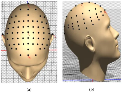
Electroencephalography has been used to study brain functioning by recording electrical activity of the neural tissue. The electrical impulses generated by the neurons in the brain, permeate the bone tissue to the scalp. These low amplitude signals across the scalp are recorded at specific sampling frequencies of 160 - 512 Hz [22]. Numerous electrodes are placed at specific locations on the scalp based on 10-10 and 10-20 placement systems. The number of electrodes can range anywhere from 1 to 128 electrodes. But most studies use a 32 or 64 electrode setup for study. In Fig 2.4, a 64 electrode EEG setup is shown where the electrodes are placed on scalp using a 10-10 positioning system. EEG signals are used to detect mental abnormalities such as sleep disorders, epilepsy, and paralysis. Due to its noninvasive and cost effective features, EEG has been used in Brain Computer
Interface (BCI) systems. Neural signals recorded by EEG are not only used to detect mental abnormalities but are now being used to transfer human thought into computer enabled action [23]. T 9 T 10 Fp z C z I z (a) Fp z Cz (b)
Figure 2.4: EEG electrode setup using 10-10 standard system a. Anterior view b. Lateral view
Signals acquired using EEG can also be represented in the frequency domain within four bandwidths. These bandwidths are categorized as alpha, beta, theta and delta. The alpha waves are rhythmic waves that exist between 8 to 13 Hz. These waves originate mostly in adults while awake and in resting state. The waves are mainly concentrated in the occipital region. At normal and attentive state, the beta waves are generated at frequencies between 14 - 80 Hz. These waves predominantly originate in the frontal and parietal regions of the brain. Theta waves are generated during emotional stress, disappointment and frustration. They also occur between 4 - 7 Hz among people suffering from degenerative brain disorders. Lastly, delta waves are generated during deep-sleep state and infancy at 3.5 Hz. These frequency bandwidths are also used to study and analyze the brain.
16
2.3
Applications of Brain Computer Interface
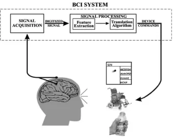
Brian computer interface (BCI), is an interface that extracts, detects, and translates specific neural generated impulses from the brain into machine defined as actions. BCI systems generally consist of three sections, acquisitioning system, feature extraction system, and signal classification system. This outline of a standard BCI system is shown in Fig 2.5. Within these three sections of the BCI system, EEG has become an effective tool to acquire brain signals from the scalp. In the second section, specific neural features that were performed by the subject triggered by specific visual or vocal queues are identified using feature extraction techniques. Some of the feature extraction techniques transform time based EEG signals to the frequency domain. And data at specific frequencies is extracted and re-transformed back into the time domain.
1034 IEEE TRANSACTIONS ON BIOMEDICAL ENGINEERING, VOL. 51, NO. 6, JUNE 2004
BCI2000: A General-Purpose Brain-Computer
Interface (BCI) System
Gerwin Schalk*, Member, IEEE, Dennis J. McFarland, Thilo Hinterberger, Niels Birbaumer, and Jonathan R. Wolpaw
Abstract—Many laboratories have begun to develop
brain-com-puter interface (BCI) systems that provide communication and control capabilities to people with severe motor disabilities. Fur-ther progress and realization of practical applications depends on systematic evaluations and comparisons of different brain signals, recording methods, processing algorithms, output formats, and operating protocols. However, the typical BCI system is designed specifically for one particular BCI method and is, therefore, not suited to the systematic studies that are essential for continued progress. In response to this problem, we have developed a documented general-purpose BCI research and development platform called BCI2000. BCI2000 can incorporate alone or in combination any brain signals, signal processing methods, output devices, and operating protocols. This report is intended to describe to investigators, biomedical engineers, and computer scientists the concepts that the BCI2000 system is based upon and gives examples of successful BCI implementations using this system. To date, we have used BCI2000 to create BCI systems for a variety of brain signals, processing methods, and applications. The data show that these systems function well in online operation and that BCI2000 satisfies the stringent real-time requirements of BCI systems. By substantially reducing labor and cost, BCI2000 facilitates the implementation of different BCI systems and other psychophysiological experiments. It is available with full documentation and free of charge for research or educational purposes and is currently being used in a variety of studies by many research groups.
Index Terms—Assistive devices, augmentative communication,
brain-computer interface (BCI), ECoG, electroencephalography (EEG), psychophysiology, rehabilitation.
Manuscript received June 25, 2003; revised February 15, 2004. This work was supported in part by the National Center for Medical Rehabilitation Re-search, National Institute of Child Health and Human Development, National Institutes of Health (NIH) under Grant HD30146, and in part by the National Institute of Biomedical Imaging and Bioengineering and the National Institute of Neurological Disorders and Stroke, NIH, under Grant EB00856, and in part by the Deutsche Forschungsgemeinschaft (DFG) and the Federal Ministry of Education and Research (BMBF).Asterisk indicates corresponding author.
*G. Schalk is with the Laboratory of Nervous System Disorders, Wadsworth Center, New York State Department of Health, Albany, NY 12201-0509 USA (e-mail: [email protected]).
D. J. McFarland is with the Laboratory of Nervous System Disorders, Wadsworth Center, New York State Department of Health, Albany, NY 12201-0509 USA.
T. Hinterberger is with the Institute of Medical Psychology and Behavioral Neurobiology, Eberhard-Karls-University of Tübingen, D-72074 Tübingen, Germany.
N. Birbaumer is with the the Institute of Medical Psychology and Behavioral Neurobiology, Eberhard-Karls-University of Tübingen, D-72074 Tübingen, Germany, and also with the Center for Cognitive Neuroscience, University of Trento, 38100 Trento, Italy.
J. R. Wolpaw is with the Laboratory of Nervous System Disorders, Wadsworth Center, New York State Department of Health, Albany, NY 12201-0509 USA, and also with the State University of New York, Albany, NY 12222 USA.
Digital Object Identifier 10.1109/TBME.2004.827072
Fig. 1. Basic design and operation of any BCI system. Signals from the brain are acquired by electrodes on the scalp, the cortical surface, or from within the brain and are processed to extract specific signal features (e.g., amplitudes of evoked potentials or sensorimotor cortex rhythms, firing rates of cortical neurons) that reflect the user’s intent. Features are translated into commands that operate a device (e.g., a simple word processing program, a wheelchair, or a neuroprosthesis).
I. INTRODUCTION A. Brain-Computer Interface (BCI) Technology
M
ANY people with severe motor disabilities needaug-mentative communication technology. Those who are totally paralyzed, or “locked-in,” cannot use conventional aug-mentative technologies, all of which require some measure of muscle control. Over the past two decades, a variety of studies has evaluated the possibility that brain signals recorded from the scalp or from within the brain could provide new augmentative technology that does not require muscle control (e.g., [1]–[8]); see [9] for a comprehensive review. These BCI systems mea-sure specific features of brain activity and translate them into device control signals (see Fig. 1, modified from [9]). The fea-tures used in studies to date include slow cortical potentials, P300 evoked potentials, sensorimotor rhythms recorded from the scalp, event-related potentials recorded on the cortex, and neuronal action potentials recorded within the cortex.
These studies show that nonmuscular communication and control is possible and might serve useful purposes for those who cannot use conventional technologies. To people who are locked-in (e.g., by end-stage amyotrophic lateral sclerosis, brainstem stroke, or severe polyneuropathy) or lack any useful muscle control (e.g., due to severe cerebral palsy), a BCI system 0018-9294/04$20.00 © 2004 IEEE
Figure 2.5: Outline of a brain computed interface system with its three main components.
To mitigate noise issues, BCI systems use digital filters or feature selection techniques to remove unwanted artifacts from the EEG data. Sole use of low-pass or band-pass filters, do not remove eye and muscle related contamination present in the signal. However in some EEG recordings for BCI system, users were asked to restrict their eye movements to minimize contamination. This approach is impractical for real world BCI applications. To
remove noise artifacts, blind source separation (BSS) models can be effective. Independent component analysis (ICA) is one such technique which has been successfully used to extract neural related features from contaminated signals [24, 25].
2.4
Artificial Neural Networks
Artificial neural network (ANN) are computation models that mimic the workings of the brain. These models were widely studied in the early eighties and nineties. However, until recently, implementation of this concept had remained a challenge due its computational cost. The ANN models work well for machine learning problems and are better adept to learning and classifying data with complex variations consisting of a large feature sets. The human brain does a marvelous job in learning new things through processing various inputs such as speaking, movement, hearing, sense of touch, sight, listening and complex motor imagery. Scientists hypothesize that brain is highly flexible and can adapt to a new input. In a study, the neural connections between the auditory nerve and the auditory cortex were severed and the optic nerve of the eye was connected to the auditory cortex. Remarkably, the auditory cortex learned to see. In another study, the somatosensroy cortex of the brain which processes the sense of touch was re-wired to receive visual inputs from the optic nerve. The somatosensroy cortex had learned to process the visual signals. These re-wiring experiments establish, that any part of the brain can be used process and learn any kind of input. This encourages researcher to explore a single computational model that can replicate brain’s processing capabilities. On a computer, accomplishing such flexibility in learning can seem challenging and to mimic the brain it is essential to introduce the neuron.
18
2.4.1 Structure of Neuron
The neuron is the main processing unit of brain and there are approximately three trillion neurons in the human brain. The structure of the neuron can be categorized into three parts, the axon, dentrites and the cell body as shown in Fig 2.6. The dentrites connect the cell
Figure 2.6: Proposed Classification System Model
body to other neurons. There can be numerous dentrites to a neuron and can extend upto 0.5 meters in length. Through dentrites signals are carried into the neuron. The axon is another extension of the cell body that is coated with a protein insulation called the Myelin Sheath. The axon is a longer extension and can measure upto one meters in length. The elongation carries signals out of the cell to the axon terminal.
2.4.2 Brief Overview of Neural Networks
Using the structure of neuron, the computational model of the artificial neural network was designed. In 1943, Warren McCulloch and Walter Pitts created a computational model of the neural network [26]. Backpropagation models were later proposed as addtions to the neural network model in 1975 [27]. Within the ANN, the neuron has one output and one input. In the neuron, the input is multiplied to a weight and fed into a transfer function. Three transfer functions are mainly used in NN systems, i.e, the hard-limit transfer function, linear transfer function and log-sigmoid transfer function. The hard-limit transfer function
19
Neuron Model
2-3 All of the neurons in this toolbox have provision for a bias, and a bias is used in many of our examples and will be assumed in most of this toolbox. However, you may omit a bias in a neuron if you want.
As previously noted, the bias b is an adjustable (scalar) parameter of the neuron. It is not an input. However, the constant 1 that drives the bias is an input and must be treated as such when considering the linear dependence of input vectors in Chapter 4, “Linear Filters.”
Transfer Functions
Many transfer functions are included in this toolbox. A complete list of them can be found in “Transfer Function Graphs” in Chapter 14. Three of the most commonly used functions are shown below.
The hard-limit transfer function shown above limits the output of the neuron to either 0, if the net input argument n is less than 0; or 1, if n is greater than or equal to 0. We will use this function in Chapter 3 “Perceptrons” to create neurons that make classification decisions.
The toolbox has a function, hardlim, to realize the mathematical hard-limit transfer function shown above. Try the code shown below.
n = -5:0.1:5;
plot(n,hardlim(n),'c+:');
It produces a plot of the function hardlim over the range -5 to +5.
All of the mathematical transfer functions in the toolbox can be realized with a function having the same name.
The linear transfer function is shown below. a = hardlim(n)
Hard-Limit Transfer Function
-1 n 0 +1 a (a) Hard-Limit
2
Neuron Model and Network Architectures2-4
Neurons of this type are used as linear approximators in “Linear Filters” in Chapter 4.
The sigmoid transfer function shown below takes the input, which may have any value between plus and minus infinity, and squashes the output into the range 0 to 1.
This transfer function is commonly used in backpropagation networks, in part because it is differentiable.
The symbol in the square to the right of each transfer function graph shown above represents the associated transfer function. These icons will replace the general f in the boxes of network diagrams to show the particular transfer function being used.
For a complete listing of transfer functions and their icons, see the “Transfer Function Graphs” in Chapter 14. You can also specify your own transfer functions. You are not limited to the transfer functions listed in Chapter 14.
n
0 -1 +1
a = purelin(n)
Linear Transfer Function
a -1 n 0 +1 a
Log-Sigmoid Transfer Function
a = logsig(n) (b) Linear
2-4
Neurons of this type are used as linear approximators in “Linear Filters” in Chapter 4.
The sigmoid transfer function shown below takes the input, which may have any value between plus and minus infinity, and squashes the output into the range 0 to 1.
This transfer function is commonly used in backpropagation networks, in part because it is differentiable.
The symbol in the square to the right of each transfer function graph shown above represents the associated transfer function. These icons will replace the general f in the boxes of network diagrams to show the particular transfer function being used.
For a complete listing of transfer functions and their icons, see the “Transfer Function Graphs” in Chapter 14. You can also specify your own transfer functions. You are not limited to the transfer functions listed in Chapter 14.
n
0 -1 +1
a = purelin(n)
Linear Transfer Function a -1 n 0 +1 a
Log-Sigmoid Transfer Function
a = logsig(n) (c) Log-Sigmoid
Figure 2.7: Types of transfer functions used in a neuron [28].
outputs is ’0’ when the input is less that zero and outputs a ’1’ when the input is greater than one. Neurons using a linear transfer function use linear approximations or linear filters to provide outputs. Finally, the log-sigmoid transfer function in neurons, takes input values between -∞and +∞and provides outputs in a range between 0 and 1. The sigmoid function is frequently used in backpropagation networks due to the differential properties. The outputs for these functions are shown in Fig 2.7. In the figure, the pre-defined MATLAB functions are also shown. Using these functions the neuron computes its output and feeds it forward to the next neuron. Along with inputs and weights, the neuron can also have a bias associated to it. The bias parameter is used to add further emphasis to the neuron’s output. The structure of a neuron is shown in Fig 2.8.
Input
bias
weight
H(x)
A = f(Input * weight + Bias)
x1
x1
x1
a1
a2
a3
x
H(x)
Θ
2
Θ
1
x0
a0
Bias Terms20
2.4.3 Feed Forward Network
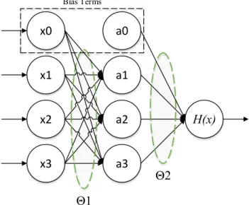
Basic ANN architecture mainly consists of three types of layers, i.e, input layer, hidden layer and the output layer. As seen in Fig 2.9, a simple ANN consists of three types of layers with several nodes, each designated to a neuron. The computation of in each layer can be
Input
bias weight
H(x)
A = f(Input * weight + Bias)
x1 x2 x3 a1 a2 a3 x H(x) Θ2 Θ1 x0 a0 Bias Terms
Figure 2.9: Feed Forward Neural Network
mathematically represented as follows.
a1 =g(θ1 10x0+θ 1 11x1+θ 1 12x2+θ 1 12x3) a2 =g(θ1 20x0+θ 1 21x1+θ 1 22x2+θ 1 23x3) a3 =g(θ1 30x0+θ131x1+θ132x2+θ331 x3) H(x)=g(θ2 10a0+θ 2 11a1+θ 2 12a2+θ 2 13a3)
where x0and a0 are bias parameters andg(x)is the transfer function. Size of the weight
matrix of the layer Θ1 consists of Sj+1 x(Sj +1)values. Here j is the number of layers
in the ANN architecture. The weight matrix changes for each layer. In Fig 2.9, the input layer consists of inputs X = {x0,x1,x2,x3}, the hidden layer nodes are denoted as
the output. In Eq 2.1, the above equations can be represented a vectorized form,
Z =Θ1∗ X (2.1)
whereΘ1is the weight matrix for the hidden layer and X is the matrix containing the input
values. Each of the nodes in the hidden layer compute an output using a transfer function
g(x)as shown in Eq 2.2,
A=g(Z) (2.2)
whereAconsists output values from all the nodes of the hidden layer. The final outputH(x) is computed in Eq 2.3,
H(x)= Θ2∗ A (2.3)
whereΘ2is the weight matrix for the output layer.
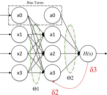
2.4.4 Cost Function & Backpropagation
While the feed forward networks contain neurons that calculate outputs based on the given input, weight and bias parameters, the backpropagation model in the neural networks optimizes a cost function and updates the weights in each layer of the neural network. Before the process of backpropagation is explained, it is necessary to introduce the cost function of a neural network model. The function is similar to the cost function of a logistic regression classifier but the cost J(Θ) in NN models is calculated for all the layers. In Eq 2.4, the cost function is defined as,
J(Θ)= −1 n © « n Õ i=1 T Õ j=1 yijlog(H(xi))j+(1−yij)log(1−H(xi))jª ® ¬ (2.4)
where n is the number of nodes in a layer, T is the number of layers, yij is the expected output of jt h node in theit h layer andH(xi)is the acquired output of the jt h node in theit h layer. Using the above cost function, the backpropagation model seek to optimize weights by minimizingJ(Θ).
22 Input bias weight H(x)
A = f(Input * weight + Bias)
x1 x2 x3 a1 a2 a3 x H(x) Θ2 Θ1 x0 a0 Bias Terms x1 x2 x3 a1 a2 a3 H(x) Θ2 Θ1 x0 a0 Bias Terms
δ3
δ
2
Figure 2.10: Backpropagation in a Feed Forward NN
In Eq 2.5, using the cost function an errorδijin each layer is calculated as, δi j =a i j−y i j (2.5)
where aij is the computed output, yij is the expected output at jt h node in the it h layer. The error in each layer is summed for all the nodes and then multiplied to the error of the previous layer. The errors are from the output layer to the input layer in a backward direction as shown in Fig 2.10. For such network, the backpropagation process is shown in as,
δ3 j = δ i j =a4j −yj δ2 j = (Θ2δ3j) ∗a2j(1−a2j) Using the computed errors the cost J(Θ)is minimized by,
δJ(Θ) δΘ =a n Tδ n T (2.6)
The key computational aspects of the research have been explained in this chapter. The proposed techniques using EEG, augmented BCI with ANN classification is explored in the next chapters.
CHAPTER 3
OPTIMIZATION OF EEG-BASED IMAGINARY MOTION CLASSIFICATION USING MAJORITY-VOTING
3.1
Overview
In this chapter, a majority-vote system was added to a network of artificial neural networks (ANN) to optimally classify imaginary motions performed by subjects for multiple sessions. The proposed technique optimizes the electrodes used for individual user classification by ranking each electrode’s data based on its individual classification accuracy. The best performing electrodes are identified with a rank-based statistical analysis. The remainder of this chapter is organized as follows. Section 3.2 discusses the EEG data used in the experiments conducted to validate the proposed method. Section 3.3 illustrates the proposed method. Section 3.4 reports the results of the proposed method. Section 3.5 introduces the genetic algorithm to optimize electrodes and seeks to further improve classfication accuracy, the findings are also compared for improvements. Finally, the results and findings obtained from these experiments are summarized in the conclusion in section 3.6.
3.2
Dataset Description
Dataset V from the BCI Competition III was used for validation. The data was recorded by the Istituto Dalle Molle di Intelligenza Artificiale Percettiva (IDIAP) research institute in Switzerland [29]. The dataset consists of brain activity pertaining to three specific tasks from three healthy male subjects. These brain signals were recorded in repeated sessions over a course of a single day and the subject’s imagination of three types of exercises included - left hand movement, right hand movement, and imagination of words starting with the same letter. Each of these three sessions lasted for 4 minutes with brief intervals ranging between 5-10 minutes. During each session, the subjects imagined a specific task
24
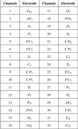
Table 3.1: Electrodes & Their Alloted Channel Numbers
Channels Electrode Channels Electrode
1 FP1 17 O2 2 AF3 18 PO4 3 F7 19 P4 4 F3 20 T6 5 FC1 21 C P6 6 FC5 22 C P2 7 T3 23 C4 8 C3 24 T4 9 C P1 25 FC6 10 C P5 26 FC2 11 T5 27 F4 12 P3 28 F8 13 PZ 29 AF4 14 PO3 30 F P2 15 O1 31 FZ 16 OZ 32 CZ
for a time period of 15 seconds and tasks were changed as indicated by the operator. The voltages across the scalp were measured using the Biosemi portable EEG machine with a sampling frequency of 512 Hz. Thirty two electrodes were used to acquire data and electrodes were placed at specific locations on the scalp using the IEEE 10-20 standard system. Electrodes were assigned a number for ease of reference and the numbers relating to the electrode names are listed in Table 4.2. The raw data from these 3 subjects over the 3 sessions comprise of 3×3×32=288 total data channels.
3.3
ANN Structure & Majority Voting System
The prime focus of this research is to implement a Majority Voting (MV) system to optimize the classification accuracy for each subject. It’s main contribution lies in the unique structure
for this classifier that utilizes a network of relatively simple ANNs with a majority vote circuit. Instead of using a single complicated ANN with 32 inputs, using majority vote simplified the ANN structure. Before the voting system is explained, it is essential to first describe the system structure. The EEG recordings for each of the three subjects contain columns of data acquired from each of the 32 channels. The data from each column is input into an artificial neural network (ANN). These neural networks use back propagation to train, test, and validate the data. In this experiment, 70% of the data was used for training, and 30% was used for testing and validation. The ANN structure has a single neuron assigned for input, while the hidden layer consists of 10 neurons in its first layer and 20 neurons in the second. The output layer was allotted 3 neurons. The outputs acquired from the neural networks were categorized by the MV system into 3 imaginary task categories i.e, class 7, class 2, and class 3.
The process is visually illustrated in Figure 3.1. The acquired ANN data is split into three columns for each of the 32 channels. Across each row of the three columns, the maximum value is replaced with a ’1’, and the rest are changed to ’0’. Next, these binary values are added to the binary values acquired from other channel’s ANN outputs. This process repeated for each row results in a single output that consists of the majority voted data from all of the specified channels.
Majority
Vote Output
... ...
26
Algorithm 1Majority-Vote Model of ANN Outputs.
Precondition: For each subject,{x1,x2, ...xn}is data fromnchannels.
1: functionMajority Vote(x1,x2, ...,xn)
2: fork ←1 tondo .Number of iterations
3: [Ak,yk] ← AN N(xk)
4: end for .Y containsyk outputs and Acontains Ak classification accuracies from
ANN.
5: {z1,z2, ...zn} ←r ank(Y)based on An. . Z hasznranked channels.
6: fori ←1 to N do . N ranked outputs considered.
7: zi ← {ai,bi,ci}
8: {{ai,bi,ci}are 3 imaginary tasks contained inzi.}
9: [r ows,columns] ←size(zi) 10: for j ←1 tor owsdo
11: zi∗←max({ai j,bi j,ci j})=1 and
12: zi∗←nonmax({ai,bi,ci})=0
13: {Row max for 3 tasks replaced with 1, others with 0.}
14: end for
15: δi← sum(zi∗)
16: end for
17: δ← {δ1, δ2, ..., δN}
18: form←1 to N do
19: M a jorityV oted←max(δm)=1 and
20: M a jorityV oted←nonmax(δm)=0
21: end for
Using the MV system, the overall aggregated classification accuracy of all 32 channels was evaluated to obtain a baseline accuracy. Next, all 32 channels were ranked based on their individual classification accuracies and then sorted in a descending order. By using the obtained ranked and sorted sequence, the channels were majority voted in an iterative process starting from the most to the least accurate channel. This process of majority voting is detailed in Algorithm 1. The process continues until the overall aggregated classification accuracy of the majority vote is optimized.
Using this process, the set of electrodes used to generate the maximum classification accuracy was considered as the optimal set for that user. To quantify the effectiveness of the proposed approach, the classification accuracies of the optimized set of electrodes for each user and the overall classification accuracy across all users were obtained and analyzed in Section 3.4.
3.4
Results & Data Analysis
Data for each subject contains 3 sessions of repeated imaginary tasks. Using the major-ity voting system, channel data for each session was ranked and sorted according to the individual ANN channel accuracies. In the channel optimization process, the majority voting process was used twice. The first time, channel optimization was performed for each session separately. Using this method, wide variations were noticed across the three sessions among the optimized channel sets for each subject. This was due to the presence of time and magnitude related variance in the input data itself. The MV accuracies across the 32 iterations are presented in Figures 3.2-(a,b,c) for all three subjects in the dataset. In these plots, the x-axis does not represent 32 separate channels but rather 32 iterations of sequential majority voting of ranked channels based on their accuracies.
In order to mitigate the fluctuations across the subject sessions and stabilize the op-timization process, the majority voting process was used again. However, this time the
28 0 5 1 0 1 5 2 0 2 5 3 0 6 0 7 0 8 0 9 0 1 0 0 1 1 3 2 2 1 5 1 6 6 2 6 1 8 7 3 2 3 12 91 2 1 51 0 3 2 31 12 52 01 7 2 23 02 4 9 1 9 8 2 71 4 4 2 8 1 9 1 8 2 32 1 2 52 72 62 2 9 3 01 1 1 7 1 3 5 3 11 2 6 1 3 7 3 2 2 2 0 1 02 8 4 1 5 8 1 4 2 92 4 1 6 2 4 2 9 2 1 3 1 4 2 8 2 5 3 0 5 1 0 7 2 7 1 7 1 91 32 0 1 11 4 2 1 6 9 3 8 1 52 3 1 1 22 6 3 2 2 2 6 1 8 A c c u ra c y ( % ) N u m b e r o f I t e r a t i o n s S e s s i o n 1 S e s s i o n 2 S e s s i o n 3 (a) Subject 1 0 5 1 0 1 5 2 0 2 5 3 0 6 0 7 0 8 0 9 0 1 0 0 8 2 3 5 3 22 4 1 1 16 1 7 2 22 53 2 42 92 17 2 81 3 1 42 01 81 53 03 19 1 91 22 72 61 01 6 8 5 3 2 2 3 1 32 21 4 6 1 53 11 2 3 02 4 1 2 12 2 71 72 62 81 83 1 99 2 91 11 07 2 02 54 1 6 5 8 2 33 2 1 2 1 31 46 1 52 12 22 53 01 02 4 1 1 72 92 87 3 12 71 61 11 92 63 9 1 82 02 4 A c c u ra c y ( % ) I t e r a t i o n s Session 1 Session 2 Session 3 (b) Subject 2 0 5 1 0 1 5 2 0 2 5 3 0 6 0 6 5 7 0 7 5 8 0 8 5 9 0 9 5 1 0 0 3 0 1 2 6 2 1 0 3 17 6 1 3 2 0 1 5 1 8 2 7 5 2 5 1 1 1 9 1 4 3 1 2 2 9 2 2 2 8 8 1 6 2 3 2 1 3 2 4 9 2 4 1 7 1 0 2 3 0 1 4 2 3 1 2 0 2 4 1 2 9 2 2 1 5 2 9 1 6 2 61 12 81 3 2 12 7 7 1 9 5 3 2 1 7 4 6 3 1 3 1 8 8 2 5 1 4 2 4 1 0 1 5 1 3 1 6 2 0 2 1 1 21 7 3 2 32 11 83 22 8 8 9 5 7 6 4 2 91 12 7 2 62 53 03 12 21 9 A c c u ra c y ( % ) N u m b e r o f I t e r a t i o n s S e s s i o n 1 S e s s i o n 2 S e s s i o n 3 (c) Subject 3
Figure 3.2: Accuracies for Sequential Majority Voted Channel Combinations based on Ranked Individual Channel Accuracies for each of the three Sessions.
individual channel accuracies for each session were averaged and then sorted in decreasing order. The channel sequence obtained was input into the majority voting system. The aver-aged ANN accuracies for each channel is shown in Figures 3.3-(a,b,c) for the three subjects. Their ranks are also specified in the figure. Using these ranks, the MV system evaluated the classification accuracies for each session. The resulting MV accuracies from the 32 iterations were averaged to get the final individual accuracies for each of the subjects. The
1 8 2127 3 1710 32 23221628 4 3130 1814 57 25 2 24 12 20 9 6 15 29 191311 26 0 5 10 15 20 25 30 40 50 60 70 80 90 100 A cc ur ac y (% ) Channel (a) Subject 1 109 22 15 2 5 25 1 3026 16 13 7 8 11 32 12 2827 31 14 6 4 23 18 2924 19201721 3 0 5 10 15 20 25 30 40 50 60 70 80 90 100 A cc ur ac y (% ) Channel (b) Subject 2 42 23 31 2013 10 3027 1 1511 9 5 7 17 32 22 26 6 2524 1214 28 8 182119 3 16 29 0 5 10 15 20 25 30 40 50 60 70 80 90 100 A cc ur ac y (% ) Channel (c) Subject 3
Figure 3.3: Individual Channel Classification Accuracy Averaged Across all 3 Sessions for each Subject and their Respective Rank.
highest accuracy value was considered and the channel combination sequence associated with that accuracy was considered as the optimized channel set for the specific subject. Using the above process, optimized channel sets were obtained for all three subjects.
In Figure 3.4, the highest accuracy can be observed at the 20th iteration, and at this iteration, the first 20 channels among the ranked channels were deemed optimal based on their individual classification accuracies. The classification accuracy of 69.83% was
30 0 5 1 0 1 5 2 0 2 5 3 0 6 0 7 0 8 0 9 0 1 0 0 1 2 1 5 1 31 82 6 1 9 2 2 5 7 3 1 2 3 3 01 72 7 1 1 6 1 62 9 2 4 3 1 0 9 2 22 03 2 4 1 22 81 51 4 8 8 5 3 2 2 3 6 2 2 1 3 1 4 2 1 1 5 1 71 2 2 1 4 1 13 02 52 82 93 1 3 2 42 7 7 1 01 91 82 6 9 2 01 6 1 0 2 3 0 1 1 42 01 52 6 1 3 7 1 2 2 3 6 2 41 13 11 62 72 9 5 2 8 1 8 3 2 22 11 9 9 2 53 2 8 4 1 7 A c c u ra c y ( % ) I t e r a t i o n s Subject 1 Subject 2 Subject 3
Figure 3.4: Subject Optimized Channel Accuracies over 32 Iterations
(a) Subject 1 (b) Subject 2 (c) Subject 3
Figure 3.5: Optimized electrode sets for each subject
achieved. However for Subject 2, a single electrode (C3) was deduced as optimal by the MV system to perform all three tasks and the classification accuracy was 94.04%. This was due to a significantly higher individual channel classification accuracy for that particular channel. Finally, electrodes for subject 3 were optimized to a set consisting of 14 electrodes with a classification accuracy of 84.56%. Table 3.2 summarizes the optimized classification accuracies of the three subjects. The reported overall accuracy calculated by averaging the classification accuracy of all subjects was 82.81% which is higher than the 79.96% accuracy obtained by optimizing a set of electrodes for multiusers [30].
Table 3.2: Electrode Optimization
Subject Classification Accuracy
1 69.83%
2 94.04%
3 84.56%
Average 82.81%
Figures 3.5-(a,b,c) illustrate the placement of these optimized electrodes for subject 1, subject 2, and subject 3, respectively. It is obvious from these results, that each subject utilized a different set of electrodes to obtain the optimal classification accuracy. For subjects 1 and 3, both sides of the brain worked together through corpus callosum with a certain side of the brain being more dominant than the other, while subject 2 was left lateralized. Based on these results, it is evident that subject 1 has prominent activity in the right side of the brain while subject 3 has shown more activity in the left part. Therefore, it can be concluded that people with certain hand affinity have elevated activity in respective brain regions. Figures 3.5-(a,c) illustrate the left-hand dominance and right-hand dominance for subject 1 and subject 3, respectively.
3.5
Further Optimization Using Genetic Algorithm
The genetic algorithm (GA) is a computational model that seeks to find a global minimum of complex function with given parameters and a user-defined cost function. Genetic algorithm has been used in a wide array of applications. In a study genetic algorithm has been used to extract complex features from EEG for BCI application and two classifier were used to classify the data to validate the effectiveness of feature extraction [31]. Features of five mental tasks extracted in this study. In another study, epileptic seizures in EEG signals were classified using wavelet transform and genetic algorithm [32]. They acquired a high
32
classification accuracy of 94.3% and 98% for normal and epileptic features respectively. Using genetic algorithm in optimizing EEG related data classification has always provided higher classification. To further enhance the classification accuracy of this study, the genetic algorithm was employed to the majority voting procedure. Before the process is explain in much detail, the parameters of the genetic algorithm need to be introduced.
Table 3.3: Genetic Algorithm Parameters
GA Options Description Values
Creation Function Creates the initial population. In this case, a random 32-bit [0,1] was created that was used as initial chromosomes.
Crossover Fraction Fraction by which the population characteristics are carried 0.8 to the next generation.
Crossover Function Used to create new chromosomes from the parent chromosomes Default for each generation.
Elite Count Positive integer value that guarantees the amount of chromosomes 0.05 survive to the next generation
Max Generations Maximum number of generations the GA can run 30
Population Size Size of the population 64
Mutation Function This function adds mutations for the GA to come out of local Default minima
The parameters in in Table 3.3, the parameters that were focused are listed along with their description. The algorithm had a creation function that created 64-bit long strings of rendom ’0’ and ’1’. Thirty strings were created for the initial population. These strings were used to choose the electrode data to be used in the majority voting procedure. The majority-voting was used as a cost function. Based on the output accuracy of the majority vote, the chromosomes in the GA were chosen in each generation. The genetic algorithm was set to stall after 30 generations. In this manner, the genetic algorithm was used to optimize the data for all the three subjects in the dataset. From the acquired results of the output, it was noticed that the GA was able to reduce number of electrodes required for
computation by more than 50% in subject 2 and 3. The optimized electrode positions are shown in Fig 3.6 for all the three subjects.
(a) Subject 1 (b) Subject 2 (c) Subject 3
Figure 3.6: Optimized electrode sets for each subject
For subject 1, electrodes were reduced by 50% and classification accuracy was im-proved by an average of 2.51% across all three sessions. Electrode for subject 2, were also reduced by 65.62%. This percent was computed based on the 32 electrodes and not on the results acquired through majority voted results. Accuracy was improved by 0.218% across all the three sessions. Finally for subject 3, the electrodes were optimized to a total of 12 electrodes which is a 62.50% reduction in the number of electrodes used. The classification accuracy was improve by an average of 1.9%. The optimized electrode sets and classification accuracies for each subject can be seen in Table 3.4.
Table 3.4: Weight Factors & Overall Classification Accuracy of the High & Low Groups
Optimized Electrode GA - Optimized Majority-Vote Improvement Channel
Set Accuracy (%) Accuracy (%) (%) Reduction
Subject 1 1 2 5 7 10 13 18 19 20 21 23 24 25 29 30 31 72.35% 69.83% 2.51% 20%
Subject 2 1 4 5 8 10 18 22 23 29 30 32 94.25% 94.04% 0.218% -9.09%
Subject 3 1 2 9 10 13 14 17 23 24 29 30 31 86.414% 84.56% 1.9% 40%
34
3.6
Summary
In this chapter, majority vote system was applied to a system of neural networks in order to optimally classify three imaginary tasks performed by three subjects. This proposed approach optimized the electrodes for each individual user by ranking the electrodes based on their individual classification accuracies. Averaging the electrode accuracies reduced the variance across the sessions and by implementing the majority vote the best performing electrodes are shortlisted for each user. It was observed that using a network of simple neural networks along with the majority vote system improved the classification accuracy of each subject significantly. In addition, the averaged overall classification accuracy of all three subjects increased from 79.96% to 82.81%. Using the genetic algorithm, the acquired accruacy from the majority vote was further optimized to 84.34% which is 1.56% greater. The number of electrodes used in the computation was also reduced by more than 50% with this process. In this work it can concluded that not only accuracy was improved but also the computation time was effective reduced through electrode optimization by using majority voting and genetic algorithm. By this it is evident that classification accuracy is user-dependent and hence each user has a different set of optimal electrodes. To further validate and investigate this technique, the majority voting system should be tested on a much larger EEG dataset.
CHAPTER 4
A COMPREHENSIVE STUDY OF MOTOR IMAGERY EEG-BASED CLASSIFICATION USING INDEPENDENT COMPONENT ANALYSIS AND
ARTIFICIAL NEURAL NETWORKS
4.1
Overview
In this chapter, robust technique is proposed that combines the use of an automatic feature extracting independent component analysis (ICA) system with an ANN classifier that uses the Levenburg-Marquardt training function to classify a large scale dataset of 105 subjects. The work validates the relationship between signal to noise ratio (SNR), signal variance across multiple sessions, and signal classification accuracy. The dataset considered for this work was acquired from PhysionNet and consists of both imagined and actual movements performed by 105 subjects. In a different study, wavelet transform features were extracted from the EEG Movement/Imagery dataset and an ANN was used for classification. This study reported a maximum classification accuracy of 68.21%. A phase locking value system (PLV) was used for the same dataset to classify the β (12-30 Hz) and µ(8-12 Hz) rythms for actual movements (78.9


![Figure 2.7: Types of transfer functions used in a neuron [28].](https://thumb-us.123doks.com/thumbv2/123dok_us/421811.2548416/24.918.211.726.110.262/figure-types-transfer-functions-used-neuron.webp)