Collaborative Recurrent Neural Networks for
Dynamic Recommender Systems
Young-Jun Ko youngjun.ko@epfl.ch
Lucas Maystre lucas.maystre@epfl.ch
Matthias Grossglauser matthias.grossglauser@epfl.ch
´
Ecole Polytechnique F´ed´erale de Lausanne, Switzerland
Editors:Robert J. Durrant and Kee-Eung Kim
Abstract
Modern technologies enable us to record sequences of online user activity at an unprece-dented scale. Although such activity logs are abundantly available, most approaches to recommender systems are based on the rating-prediction paradigm, ignoring temporal and contextual aspects of user behavior revealed by temporal, recurrent patterns. In contrast to explicit ratings, such activity logs can be collected in a non-intrusive way and can offer richer insights into the dynamics of user preferences, which could potentially lead more accurate user models.
In this work we advocate studying this ubiquitous form of data and, by combining ideas from latent factor models for collaborative filtering and language modeling, propose a novel, flexible and expressive collaborative sequence model based on recurrent neural networks. The model is designed to capture a user’s contextual state as a personalized hidden vector by summarizing cues from a data-driven, thus variable, number of past time steps, and represents items by a real-valued embedding. We found that, by exploiting the inherent structure in the data, our formulation leads to an efficient and practical method. Furthermore, we demonstrate the versatility of our model by applying it to two different tasks: music recommendation and mobility prediction, and we show empirically that our model consistently outperforms static and non-collaborative methods.
Keywords: Recurrent Neural Network, Recommender System, Neural Language Model, Collaborative Filtering
1. Introduction
As ever larger parts of the population routinely consume online an increasing amount of digital goods and services, and with the proliferation of affordable storage and computing resources, to gain valuable insight, content-, product- and service-providing organizations face the challenge and the opportunity of tracking at a large scale the activity of their users. Modeling the underlying mechanisms that govern a users’ choice for a particular item at a particular time is useful for, e.g., boosting user engagement or sales by assisting users in navigating overwhelmingly large product catalogs through recommendations, or by using profits from accurately targeted advertisement to keep services free of charge. Developing appropriate methodologies that use the available data effectively is therefore of great practical interest.
In recent years, the recommendation problem has often been cast into an explicit-rating-prediction problem, possibly facilitated by the availability of appropriate datasets (e.g.,
Bennett and Lanning, 2007; Miller et al., 2003). Incorporating a temporal aspect into the explicit-rating recommendation scenario is an active area of research (e.g., Rendle,
2010;Koren,2010;Koenigstein et al.,2011;Chi and Kolda, 2012). However, concerns are increasingly being raised about the suitability of explicit rating prediction as an effective paradigm for user modeling. Featuring prominently among the criticism are concerns about the availability and reliability of explicit ratings, as well as the static nature of this paradigm (Yi et al.,2014;Du et al.,2015), in which the tastes and interests of users are assumed to be captured by a one-time rating, thus neglecting the immediate context of the rating at the instant it is issued by the user.
In contrast, the implicit-feedback scenario is advantageous due to abundantly available data that can be gathered unintrusively in the background (Rendle et al.,2009). Although methods for processing implicit feedback often only consider a static aggregate (e.g., Ko and Khan,2014), the raw data typically consist of user activity logs, i.e., sequences of user interactions with a service, and is thus a far more suitable basis for dynamic user models. Data of this form is generated in many domains where user interactions can range from navigating a website by following links, to consuming multi-media content on a streaming site or to announcing the current physical locations on social media, thus making appropriate methods widely applicable. Moreover, a user’s behaviour is intimately linked to the context in which it is observed: factors such as mood, current activity, social setting, location, time-of-day etc. can temporarily cause a shift in a user’s item preferences. While the relevant contextual factors themselves are hard to observe or even to define, their effect might be visible in the form of particular temporal patterns in the activity logs, the exploitation of which would then lead to more fine-grained and accurate user models. The purpose of this work is therefore to develop and evaluate methods for analyzing activity sequences generated by a heterogeneous set of users.
In the remainder of this section, we will introduce the problem more formally, state the contributions in the context of related work and outline the rest of the paper.
1.1. Preliminaries
Let U denote a set of users of cardinality |U | = U and let I denote a set of items of cardinality |I|=I. As usual, the sets of users and items are assumed to be fixed. We use indices uand ito refer to users and items, respectively. For every user u∈ U we observe a sequence x(u) = [x(1u), . . . , x(Tu)
u] with elements x (u)
t ∈ I, i.e., each event in a user sequence
is an exclusive choice over the set of items. We will refer to a user making such a choice as consuming the item. Simlar to (Rendle et al., 2010), we focus on sequences without taking into account the absolute time at which the events occurred, because here, we are interested in exploiting temporal patterns expressed by the ordering of events1. We denote by x(<tu) = [x1(u), . . . , x(tu−)1] and x(≥ut) = [xt(u), . . . , x(Tu)
u] subsequences up to and from index t,
respectively.
The basic query a sequence model should support is the quantification of the likelihood of a user u to consume items at t = k, k+ 1, k+ 2, . . . given access to the history x(<ku) of events.
Our approach for such prediction tasks is to model the observed sequences probabilisti-cally. Given the ordering imposed by time, it is reasonable to choose a factorization of the joint distribution over a sequence that respects that order:
Pθ(x(u)) = Tu Y t=1 Pθ(x (u) t |x (u) <t), (1)
whereθ denotes a set of model parameters.
As we model a discrete set of outcomes, the conditionals are multinomial distributions overI, represented by probability vectorsp(tu) of dimensionI, whose concrete parameteri-zation and form is determined by the assumptions that underlie a particular model:
Pθ(x(tu)|x (u) <t) =p (u) t (θ,x (u) <t). (2)
The evaluation metric we report is the average negative log likelihood computed for a held-out part of the sequence: For every user, we splitx(u) intox<r(u)u andx(≥ur)
u at 1< ru≤
Tu and define the error as
E(x(1)≥r 1, . . . ,x (U) ≥rU |θ) =− 1 U X u∈U 1 Tu−ru+ 1 logPθ(x (u) ≥ru). (3)
The desired traits of a model for this kind of data are (1) flexibility, (2) the ability to model complex, potentially long-range dependencies in the sequences, and (3) collaboration between users.
Flexibility. Although we often have at our disposal datasets richer than the sequences described above, these sequences are a common denominator for many applications. Thus, we devise practical methods suitable for processing sequences, but with the flexibility for handling different tasks with minor modifications, ideally in an end-to-end fashion, and for tapping into existing sources of metadata to augment the sequences.
Long-range Dependencies. The model needs to be powerful enough to represent com-plex dependencies within long sequences that might be of different length, in contrast to methods that, in order to achieve scalability, have to make compromises regarding the number of past events taken into account (Rendle et al.,2010;Wang et al.,2015).
Collaboration. Conceivably, there are two extreme cases: each individual user’s behavior is modeled in isolation, or all users are described by a single prototypical behavioral profile. There are several drawbacks to both extremes: the former approach clearly relies on the sufficient availability of observations about each user, whereas realistically, the distribution of ratings over users is often heavily skewed in favor of a few very active users. Furthermore, users typically only access a subset of the items, thus making it difficult to recommend anything outside of this subset in a data-driven way. The latter approach, i.e. ignoring to the concept of individual users, lies on the other end of the spectrum and implies that all
sequences are pooled together. Although pooling mitigates the sparsity problem, it is a strong assumption that neglects potentially important differences in user behavior. Neither extreme satisfies the assumptions we stated previously. Instead, our model needs to be personalized yet collaborative to make efficient use of the available data by identifying parameters that can be learned across users.
In this work, we develop a model that fulfills these requirements based on recurrent neural networks (RNN, Rumelhart et al.,1988;Werbos,1990).
1.2. Contributions
Using ideas from language modeling and the collaborative-filtering literature, we propose a novel collaborative sequence model that, based on RNNs, makes efficient use of the multi-user structure in the data. We study different architectural variants of our model and find that including the collaborative aspect can lead to an efficient, practical method. To test the viability of our approach, we conduct a broad empirical study on two very different real-world tasks. We find that the new model significantly outperforms various baseline methods.
Related Work. As previously mentioned, there has been much work dedicated to the rating-prediction problem. Some of these methods also take into account the effect of time (Rendle,2010;Koren,2010;Koenigstein et al.,2011;Chi and Kolda,2012). The difference is that recurrent temporal patterns are not apparent in the underlying datasets, because ratings are one-time events. Du et al.(2015) propose a model for recurrent user activities, but use a fundamentally different approach: they use continuous-time stochastic processes to explicitly model time and tie the recommendation to a specific point in time and focus more on modelingwhen the next event might occur by using the self-excitation property of the Hawkes process. A problem closely related to our setup is the next-basket prediction for e-commerce applications (Rendle et al., 2010; Wang et al., 2015), which models sequences of sets of items that represent the contents of shopping carts bought by users. Wang et al. (2015) learn a hierarchical latent-factor representation reminiscent of a multi-layer perceptron arguing that the non-linearity in their model is a crucial component. Rendle et al. (2010) use a Markov chain per user and assume low-rank structure for the transition tensor and optimize a BPR-inspired objective (Rendle et al., 2009). Our work differs in mainly two ways: first, we model events at a finer granularity, i.e., per event, which is more appropriate for the applications we considered. Second, the use of RNNs enables us to model long-range dependencies, whereas their models use much stricter factorzation assumptions for computational reasons. To the best of our knowledge, this is the first use of RNNs in this context.
Outline. This paper is organized as follows. In Section 2, we begin by motivating our approach and then presenting various baseline methods that comply with our framework. Next, we introduce RNN-based language models that serve as the basis for our collaborative RNN model. We describe the learning algorithm we use and architectural variants. We present the experimental evaluation in Section 3. In Section 4, we summarize and discuss our work and give an outlook on future extensions.
2. The Collaborative Recurrent Neural Network Model
We adopting a generative view on sequences and in the same spirit as latent factor models (Koren et al., 2009) and word embeddings (Mikolov et al., 2013), we postulate a latent feature embedding that characterizes the items and that can be considered static for the time-scale of interest. Then, it is plausible that a user’s subsequent choice is determined by the user’s internal state, describing her current valuation of the item features. This internal state is hidden and can only be inferred from recent activity and could be due to a mechanism too complicated to explicitly describe. Recurrent neural networks are powerful sequence models that operate in precisely this way: They maintain a hidden state that is updated by a complex, non-linear function learned from the data itself when the next element in the input sequence is presented to the network.
In recent years, practical advances in the area of recurrent neural networks and their variants (Hochreiter and Schmidhuber, 1997; Cho et al., 2014b) have led to enormously successful methods to tackle various interesting, yet extremely challenging, tasks that are inherently sequential in nature, most prominently in, but not restricted to, the area of Nat-ural Language Processing (NLP). The success of RNN-based models in these applications demonstrates their versatility, flexibility and ability to capture complex patterns that re-quire the model to retain information gathered at various previous time steps, possibly in the distant past. Therefore, in spite of shortcomings such as the lack of theoretical guar-antees on the performance, we deemed RNNs to be a solid foundation on top of which we developed a model that fulfills the previously posed requirements.
Next, we briefly present the RNN Language Model (RNNLM, Mikolov et al.,2010) in Section 2.2, the main source of inspiration for this work, as we find their formulation to closely match our setup. In their setup, I represents the vocabulary, and user sequences are sentences. The crucial difference to our setup is that the goal in language modeling is to learn asingle underlying concept that ties together all sequences: a generative model for the language. Thus, it makes sense to not seek to model the dynamics per sequence, but to do so for the whole corpus. The necessary model-complexity for capturing the nuances of a language is achieved by adding more layers (Graves et al., 2013; Sutskever et al.,2014). This perspective is to an extent supported by the type of data itself: For language models, a corpus consists of a plethora of relatively short sequences from the same language, whereas in our case, sequences are very long and are expressions of relatively few distinctly individual preferences. This difference in perspective underlies our approach in Section2.3.
2.1. Baseline Models
Many approaches to specify a model within the framework of Eq.1come to mind. Here, we present several straightforward models, that differ on whether or not they have a mechanism to represent dynamics and collaboration, and against which we will benchmark our method.
Static Uniform. As a trivial example, consider the uniform distribution over I. P(x(tu)|x<t(u)) =P(x(tu)) = 1
I. (4)
n-grams. n-gram models, popular in NLP (Brown et al., 1992), are distributions over co-occurrences of n consecutive items and thus have to maintain O(In) parameters. Due
to data sparsity, we consider only n = 1 (unigram) and n = 2 (bigram). We define the following quantities: ci = X u∈U Tu X t=1 1(x(tu)=i), bij = X u∈U Tu X t=2 1(x(tu) =i, xt(−u)1=j). (5)
Then, we define the unigram model as
P(x(tu)=i|x(<tu)) =P(x(tu)=i) = P ci+
k∈I(ck+)
. (6)
Similarly, the bigram model is defined as
P(x(tu)=i|x<t(u)) =P(xt(u) =i|xt(−u)1 =j) =P bij+
k∈I(bkj+)
, (7)
where we added Laplace-smoothing parameterized by .
Matrix Factorization. Methods based on matrix factorization have become a widely used tool for collaborative filtering due to their early success for recommender systems (Koren et al.,2009). Although the low-rank representation of a rating matrix is helpful for sparse static rating data by transferring knowledge between similar users and items, they are less suitable for sequential data. Approaches, such as tensor factorization (Pragarauskas and Gross,2010;Chi and Kolda,2012) generalize matrix factorization to more than two dimen-sions, one of which can be used to represent time under the assumptions that observations per user are temporally aligned. Related to this issue is the a-priori unknown optimal size of time slices for grouping together related observations. These challenges could greatly increase the complexity of the model or of the processing pipeline. Nevertheless, a static method based on matrix factorization is an interesting baseline to compare against in order to study the effect of a collaborative component in isolation. From the sequential data, we construct a matrix of log-counts2, i.e., we construct a (sparse) matrix M with entries miu = log
c(iu)+ 1. Then, we compute the low-rank decomposition of M ≈VTU with
V ∈RD×I andU ∈
RD×U by solving the weighted-λ-regularized formulation byZhou et al.
(2008): min U,V X (i,u):miu>0 miu−vTi uu 2 +λ X u∈U dukuuk2+ X i∈I dikvik2 ! , (8)
where with a slight abuse of notation, we denote by du = Pi∈I1(miu > 0) and di =
P
u∈U1(miu>0). Next-step distributions can then be defined as
P(x(tu)|x<t(u)) =P(xt(u)) =g(zu), zu =VTuu, (9) g(z) = ( exp(zi) P jexp(zj) ) ∀i . (10)
2. We use log counts to combat over-dispersion due to the heavy-tailed nature of the data. Note that as a side effect the output of the softmax (Eq.9) can then be intepreted as a ratio of pseudo-counts.
This model is collaborative and makes the whole set I accessible for each user, but it neglects the sequential nature of the data.
Hidden Markov Model (HMM). Another natural candidate for comparing against is the HMM. We consider a standard formulation and refer toRabiner and Juang (1986).
2.2. The RNN Language Model (RNNLM)
Generally, RNNs compute a mapping from the input sequence to a corresponding sequence of real-valued hidden state vectors of dimensionD:
RNN ([x1, . . . , xT]) = [h1, . . . ,hT], ht∈RD. (11)
The hidden state is a very flexible representation that enables us to use the network for different tasks by defining an appropriate output layer on top. To obtain a multinomial distribution over the next item, we can simply apply a matrix Wout ∈RI×D and pass the
output vector yt∈RI through the softmax functiong(·) from Eq. 10:
yt=Woutht, (12)
P(xt|x<t) =g(yt). (13)
The ability of RNNs to model sequences comes from explicitly representing dependencies between hidden states at different times. In graphical terms, they are a generalization of the directed, acyclic graph structure of feed-forward networks by allowing cycles to represent dependencies on the past state of the network. The RNNLM (Mikolov et al., 2010) uses a simple network architecture3 that goes back to Elman (1990) and expresses the past dependency through the following recursive definition of the hidden state vectors:
at=Whht−1+Winδxt, (14)
ht=f(at). (15)
The recurrence is initialized by a constant vector h0 with small- or zero components. The matrices Wh ∈ RD×D and Win ∈ RD×I are parameters of the RNN and f(·) is a
non-linear function that is applied element-wise to its input, such as the logistic sigmoid, the hyperbolic tangent or, more recently, the rectified linear function. The input is presented to the network as one-hot encoded vectors denoted byδxt, in which case the corresponding
matrix-vector productWinδxt reduces to projecting out thext-th column ofWin. Note, that
the network can be trivially extended to accept arbitrary side information that characterizes the input at timet.
Parameter Learning. We focus on how RNNLM processes a single sequence as we will use this procedure as a building block later on. For the loss functionMikolov et al. (2010) use the log-probability of sequences (see Eq. 1), which is differentiable with respect to all parameter matrices. The network is trained using backpropagation through time (BPTT,
Williams and Zipser,1995). BPTT computes the gradient by unrolling the RNN in time and by treating it as a multi-layer feed-forward neural network with parameters tied across every
layer and error signals at every layer. For computational reasons, the sequence unrolling is truncated to a fixed sizeB. This is a popular approximation for processing longer sequences computationally more efficiently. This method is summarized in Algorithm1. To train on a full corpus, Algorithm1is used on individual sentences in a stochastic fashion. The learning rule in the original RNNLM is a gradient descent step with a scalar step size4. The training process is regularized by using early stopping and small amounts of Tikhonov regularization on the network weights.
Algorithm 1 processSequence()
Input: Sequence x,θ ={Win,Wh,Wout}, batch sizeB
Output: Updated parametersθ
1: B ←Split x into sub-sequences of lengthB
2: h0←1
3: forb∈ B do
4: h1, . . . ,hB ←RNN (b,h0;θ) (Forward pass using Eq. 15)
5: ∇θlogE ←BPTT (b,h1, . . . ,hB;θ) (Backward pass, see Appendix A) 6: θ ←LearningRule (∇θ,θ)
7: h0 =hB 8: end for
2.3. The Collaborative Recurrent Neural Network (C-RNN)
We explained previously that our model needs to represent hidden contextual state that can vary per user:
C-RNN[x(1u), . . . , x(Tu) u] = hh(1u), . . . ,h(Tu) u i , h(tu) ∈RD. (16)
Using a RNNLM-type network per user would result in several problems: the limitations to individual item libraries and excessive, potentially redundant, parameterization, with potentially insufficient data to learn the parameters effectively. Concretely, we would have to handle O(2DIU+U D2) parameters, where the problem stems from the IU term as in generalDI.
We propose the following compromise: the input and output parameter matrices Win
and Wout can be thought of as real-valued embeddings, akin to latent factors in matrix
factorization models (Koren et al.,2009) or word embeddings (Mikolov et al.,2013). With this interpretation, we assume that such latent factors embody certain global traits of items, valid across users and static on the time-scale of interest, and we attribute the dynamics to users by maintaining per-user the part of the model responsible for capturing the dynamics, i.e., the relatively small matrixWh. The parameterization is thus reduced to
a more tolerable5O(2DI+U D2), i.e.,θ =nWin,Wout,Wh(1), . . . ,W
(U)
h
o
. Correspondingly, the forward equations become personalized:
4. There are more nuances to their algorithm, but for the purpose of our development this basic exposition is sufficient.
at(u)=Wh(u)h(t−u)1+Winx(tu), (17)
h(tu)=f(a(tu)) (18)
y(tu)=Wouth(tu), (19)
P(x(tu)|x<t(u)) =g(y(tu)). (20)
Regularization and Learning Algorithm. We train the network by using Algorithm
2 that uses the BPTT procedure from Algorithm1 as a building block. For the learning rule, we found it more effective to use RMSprop (Tieleman and Hinton, 2012). For the regularization, we use early stopping and dropout (Srivastava et al., 2014), following the insights about its application to RNNs presented by Zaremba et al. (2014). Similarly to
Jozefowicz et al. (2015), we initialize the weights by randomly drawing each component i.i.d. from N(0, D−1).
Algorithm 2 Collaborative RNN Training
Input: Sequences x(1), . . . ,x(U), Batch sizeB
1: Initθ =
n
Win,Wout,Wh(1), . . . ,Wh(U)
o
2: repeat
3: R=randperm(U) (process users in random order)
4: for u∈ R do 5: θu ← n Win,Wout,Wh(u) o 6: Win,Wout,Wh(u)←processSequence x(u),θu, B (Algorithm1) 7: end for
8: untilEarly Stopping Criterion holds
2.4. Variants
Recently, since the RNNLM was first introduced, great strides have been made in the area of RNNs. Special attention has been paid to the fact that RNNs are known to be difficult to train due to vanishing and exploding gradients (Hochreiter et al.,2001).
Among the approaches to mitigating this issue (Pascanu et al., 2012; Mikolov et al.,
2014), architectural modifications to the standard RNN stand out as being easily adoptable and effective in practice. The Long Short-Term Memory (LSTM) cell introduced by Hochre-iter and Schmidhuber (1997) is the first and best-known variant, specifically designed to counteract the vanishing-gradient problem by including a gating mechanism to enable the network to retain information in a data-driven way. This method is especially appealing as it requires virtually no modifications to standard stochastic gradient descent-based learning techniques, but this comes at the cost of an increased parameterization.
In this work, we choose to use the Gated Recurrent Unit (GRU, Cho et al., 2014a), a simplified architecture that is similar in spirit to the LSTM cell and that works well in
practice (Jozefowicz et al.,2015). The forward equations for the Collaborative GRU are z(tu) =σ Wzh(u)h(t−u)1+Wzixt , (21) r(tu) =σWrh(u)h(t−u)1+Wrixt , (22) ˜ h(tu) =g(Wh(r(tu)◦h (u) t−1) +Winxt), (23) ht(u) = (1−zt(u))◦h(t−u)1+z(tu)h˜(tu). (24) Therefore, the number of parameters is increased by a small factor toO(4DI+ 3U D2).
2.5. Implementation Details
We implement the learning algorithm by using Theano (Theano Development Team,2016) and execute the code on NVIDIA Titan X GPUs on Intel Xeon E5-2680 servers with 256 GB of RAM. As we back-propagate on the fixed-sized sub-segments of the original sequence6, we can unroll the Theano scan operation, trading a minor increase in compilation time for significant speedups in execution.
3. Empirical Evaluation
In this part, we present our experimental findings. We begin by introducing the datasets that we use in Section3.1 and then address the following points. In Section3.2, we inves-tigate the influence of the RNN architecture, as well as that of the collaborative aspect of the model in contrast to the user-agnostic version. In Section3.3, we show the comparison against various baselines. Lastly, in Section 3.4 we shed some light on the difficulty of the problem by characterizing the dependence of the performance on properties of the user profile.
3.1. Datasets
We used two publicly available datasets for our evaluation: Brightkite7 (BK) and LastFM8 (LFM).
Brightkite, discontinued in 2011, used to be a location-based social network where users could actively announce (“check in”) their location and find their nearby friends. For our purposes, we focus on the check-in logs consisting of triplets of the form (user id, location id, check-in time).
The LastFM9 dataset consists of sequences of songs played by a user’s music player collected by using a tracking plug-in. In our evaluation, we consider the sequences of artists.
We apply the following preprocessing steps: AsRendle et al.(2010), we start with a 10-core subset10 and remove pathologically homogeneous user profiles (e.g., overall reporting
6. In our experiments we use a window of length 128. 7.https://snap.stanford.edu/data/loc-brightkite.html
8.http://www.dtic.upf.edu/~ocelma/MusicRecommendationDataset/lastfm-1K.html 9.http://last.fm
only a single place but hundreds or thousands of times). We prepare test sets that consist of the last 2.5% of the data clipping their length to the interval [3,500]. Additionally, in the case of LFM, we restrict the maximum sequence length to 5120, because we did not find qualitative differences beyond that length. The set of items I is taken to be the union of the individual training sequences. The resulting datasets, along with the error of a uniform baseline predictor, are summarized in Table1. We see that the total number of events of the two datasets differ by an order of magnitude, suggesting that results on the LFM dataset might be more meaningful.
Users Items Events EUnif.
BK 1 679 23 243 599 618 10.05
LFM 954 48 188 4 320 170 10.78
Table 1: Summary of the datasets. EUnif. is the negative log probability assigned to a
sequences by the uniform baseline given in Eq. 4.
3.2. Comparison of RNN Variants
The aforementioned difficulties in training RNNs has sparked numerous architectural vari-ants of the basic tanh RNN. Understanding their effect on performance is an interesting aspect in its own right with major relevance for practitioners. Therefore, e.g., Jozefow-icz et al. (2015) conducted large empirical studies comparing many thousands of variants, focusing on modifications of the original LSTM cell (Hochreiter and Schmidhuber, 1997) in comparison to the GRU (Cho et al., 2014b). Although they did not idenfify a single best model, they corroborated the observation that such advanced RNN architectures as the GRU and LSTM outperform the tanh RNN. We choose GRUs over LSTMs for their simpler formulation and parameterization and state-of-the-art performance for many tasks, and we compared it to the collaborative tanh RNN (C-tanh). We found that the advantage of the gated version over the basic RNN carries over to our setup.
Furthermore, we compared our collaborative model to the user-agnostic GRU model that we will refer to as pooled RNN (P-RNN). It is conceivable that a RNN with a large-enough number of hidden units can eventually capture even distinct, user-specific patterns. However, we found that for our problem the collaborative RNN, taylored to the structure of the problem, is far more efficient in terms of computation. This is due to the fact that, whilst the collaborative RNN maintains recurrent connection matrices per-user thus more parameters in absolute numbers, each of these matrices can be of smaller dimension. As the learning algorithms are otherwise virtually equivalent, the pooled model incurs a major performance hit. At this point, we do not rule out that the P-RNN can match the collaborative version. But with the large running times required, due to the large number of hidden units required to come close to the performance of the collaborative model, thorough model selection for even higher-dimensional models becomes extremely cumbersome. We summarize these findings in Figure 1.
In a side note, another advantage of the collaborative model, apart from the com-putational aspect, is that it meets the potential requirement of discovering user specific embeddings.
P-GRU C-tanh C-GRU
BK 6.45 6.08 6.02
LFM 4.58 4.90 4.51
0
500
1000
1500
2000
2500
Time per Epoch (seconds)
C-GRU@128 C-tanh@256
P-GRU@768
Figure 1: Left: Errors of different RNN models on the two datasets. Right: Running time comparison of a single Epoch of different RNN models on the larger LFM dataset, demonstrating the difference in the number of hidden units for each model to perform well. We found that the P-RNN achieves a similiar performance requiring an excessive amount of hidden units (D = 768). The negative impact on running time prevented us from exploring even higher-dimensional models.
3.3. Baseline Comparison
In this part, we present the comparison of our model against the various baselines that we introduced earlier. The static methods, i.e., those that do not take into account time (unigram, matrix factorization), do not perform very well, whereas the simple bigram model does (Table2).
For HMM we used the GHMM11 library and for MF we used the parallel coordinate descent algorithm byYu et al.(2012) implemented in the libpmf12 library.
1-gram MF HMM 2-gram C-GRU
BK 9.53 9.40 8.81 6.73 6.02
LFM 8.60 8.86 7.66 5.87 4.51
Table 2: Comparison with baseline methods on different datasets.
3.4. Characterization of Error
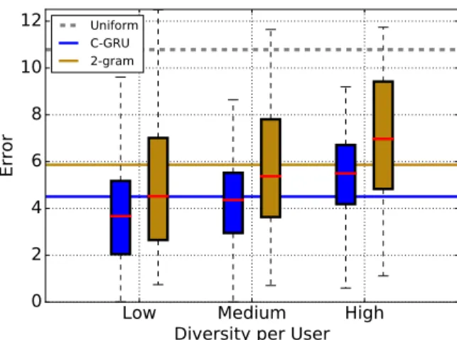
To conclude this section, we examine the error incurred on individual users and relate it to a notion of difficulty. An intuitive way to quantify the difficulty of predicting the behavior of a user is to use the Shannon entropy of the empirical distribution of items. A lower value corresponds to a lower difficulty with a lower bound of 0, which corresponds to a user having consumed the same item at all times. We divided users into three equally sized bins, according to the entropies of their sequences; in Figure2we show the distribution of errors in each bin. Unsurprisingly, there is a distinct correlation between our proxy for difficulty and the median error. We see that the C-RNN not only outperforms the closest competing baseline on average, but also in terms of variability of the errors over all bins.
11.http://ghmm.org
Low
Medium
High
Diversity per User
0
2
4
6
8
10
12
Error
Uniform C-GRU 2-gramFigure 2: LFM: Distribution of errors per user for three different difficulty regimes. These regimes were found by dividing the users into three equally-sized groups according to the entropy of their sequences. Solid lines indicate the mean errors across all users. The dashed line is the error associated with the uniform baseline. Errors are correlated with difficulty. The RNN-based model appears to not only incur a lower error on average, but also to perform more consistently.
4. Conclusion
We presented a novel collaborative RNN-based model to analyze sequences of user activity useful for modern recommender systems based on specific assumptions and modeling goals. We empirically showed that these models consistently outperform straightforward baseline methods on two real-world datasets. The model is practical in that it can be scaled to large datasets by using techniques such as those ofChen et al.(2015) for the sub-linear evaluation of the output layer in case of large item sets, or those of Recht et al. (2011) to parallelize training.
Future Work. We would like to investigate ways to incorporate into the model the abso-lute time that, in the case of activity logs, can be assumed to be available. One way could be to augment the input by the time passed since the last event. Another way could be to introduce a special symbol (similar to an end-of-sequence or unknown-word symbol in language models) to indicate a gap.
Acknowledgments We thank Holly Cogliati-Bauereis for careful proofreading. References
J. Bennett and S. Lanning. The netflix prize. In Proceedings of the KDD Cup Workshop 2007. ACM, 2007.
Peter F Brown, Peter V Desouza, Robert L Mercer, Vincent J Della Pietra, and Jenifer C Lai. Class-based n-gram models of natural language. Computational linguistics, 18(4), 1992.
Xie Chen, Xunying Liu, Mark JF Gales, and Philip C Woodland. Recurrent neural network language model training with noise contrastive estimation for speech recognition. InIEEE ICASSP, 2015. Eric C Chi and Tamara G Kolda. On tensors, sparsity, and nonnegative factorizations. SIAM
Journal on Matrix Analysis and Applications, 33(4), 2012.
Kyunghyun Cho, Bart van Merrienboer, Dzmitry Bahdanau, and Yoshua Bengio. On the properties of neural machine translation: Encoder-decoder approaches. In Proceedings of SSST@EMNLP 2014, Eighth Workshop on Syntax, Semantics and Structure in Statistical Translation, 2014a. Kyunghyun Cho, Bart van Merrienboer, C¸ aglar G¨ul¸cehre, Fethi Bougares, Holger Schwenk, and
Yoshua Bengio. Learning phrase representations using RNN encoder-decoder for statistical ma-chine translation. CoRR, abs/1406.1078, 2014b.
Nan Du, Yichen Wang, Niao He, Jimeng Sun, and Le Song. Time-sensitive recommendation from recurrent user activities. In Advances in Neural Information Processing Systems 28. 2015. Jeffrey L Elman. Finding structure in time. Cognitive science, 14(2), 1990.
Alex Graves, Abdel-rahman Mohamed, and Geoffrey Hinton. Speech recognition with deep recurrent neural networks. InIEEE ICASSP, 2013.
Sepp Hochreiter and J¨urgen Schmidhuber. Long short-term memory. Neural computation, 9(8), 1997.
Sepp Hochreiter, Yoshua Bengio, Paolo Frasconi, and J¨urgen Schmidhuber. Gradient flow in recur-rent nets: the difficulty of learning long-term dependencies, 2001.
Rafal Jozefowicz, Wojciech Zaremba, and Ilya Sutskever. An empirical exploration of recurrent network architectures. InProceedings of the 32nd International Conference on Machine Learning, 2015.
Young Jun Ko and Mohammad Emtiyaz Khan. Variational gaussian inference for bilinear models of count data. InProceedings of the Sixth Asian Conference on Machine Learning, 2014.
Noam Koenigstein, Gideon Dror, and Yehuda Koren. Yahoo! music recommendations: modeling music ratings with temporal dynamics and item taxonomy. In Proceedings of the fifth ACM conference on Recommender systems. ACM, 2011.
Yehuda Koren. Collaborative filtering with temporal dynamics. Communications of the ACM, 53 (4), 2010.
Yehuda Koren, Robert Bell, Chris Volinsky, et al. Matrix factorization techniques for recommender systems. Computer, 42(8), 2009.
Tomas Mikolov, Martin Karafi´at, Lukas Burget, Jan Cernock`y, and Sanjeev Khudanpur. Recurrent neural network based language model. In INTERSPEECH, volume 2, 2010.
Tomas Mikolov, Kai Chen, Greg Corrado, and Jeffrey Dean. Efficient estimation of word represen-tations in vector space. arXiv preprint arXiv:1301.3781, 2013.
Tomas Mikolov, Armand Joulin, Sumit Chopra, Michael Mathieu, and Marc’Aurelio Ranzato. Learn-ing longer memory in recurrent neural networks. arXiv preprint arXiv:1412.7753, 2014.
Bradley N Miller, Istvan Albert, Shyong K Lam, Joseph A Konstan, and John Riedl. Movielens unplugged: experiences with an occasionally connected recommender system. In Proceedings of the 8th international conference on Intelligent user interfaces. ACM, 2003.
Razvan Pascanu, Tomas Mikolov, and Yoshua Bengio. On the difficulty of training recurrent neural networks. arXiv preprint arXiv:1211.5063, 2012.
H Pragarauskas and Oliver Gross. Temporal collaborative filtering with bayesian probabilistic tensor factorization. 2010.
Lawrence Rabiner and B Juang. An introduction to hidden markov models. IEEE ASSP Magazine, 3(1), 1986.
Benjamin Recht, Christopher Re, Stephen Wright, and Feng Niu. Hogwild: A lock-free approach to parallelizing stochastic gradient descent. InAdvances in Neural Information Processing Systems, 2011.
Steffen Rendle. Time-variant factorization models. In Context-Aware Ranking with Factorization Models. Springer, 2010.
Steffen Rendle, Christoph Freudenthaler, Zeno Gantner, and Lars Schmidt-Thieme. Bpr: Bayesian personalized ranking from implicit feedback. In Proceedings of the Twenty-Fifth Conference on Uncertainty in Artificial Intelligence, 2009.
Steffen Rendle, Christoph Freudenthaler, and Lars Schmidt-Thieme. Factorizing personalized markov chains for next-basket recommendation. InProceedings of the 19th International Confer-ence on World Wide Web. ACM, 2010.
David E Rumelhart, Geoffrey E Hinton, and Ronald J Williams. Learning representations by back-propagating errors. Cognitive modeling, 5(3), 1988.
Nitish Srivastava, Geoffrey E Hinton, Alex Krizhevsky, Ilya Sutskever, and Ruslan Salakhutdinov. Dropout: a simple way to prevent neural networks from overfitting. Journal of Machine Learning Research, 15(1), 2014.
Ilya Sutskever, Oriol Vinyals, and Quoc V Le. Sequence to sequence learning with neural networks. InAdvances in Neural Information Processing Systems, 2014.
Theano Development Team. Theano: A Python framework for fast computation of mathematical expressions. arXiv e-prints, abs/1605.02688, May 2016.
Tijmen Tieleman and Geoffrey Hinton. Lecture 6.5-rmsprop: Divide the gradient by a running average of its recent magnitude. COURSERA: Neural Networks for Machine Learning, 2012. Pengfei Wang, Jiafeng Guo, Yanyan Lan, Jun Xu, Shengxian Wan, and Xueqi Cheng. Learning
hierarchical representation model for nextbasket recommendation. In Proceedings of the 38th International ACM SIGIR Conference on Research and Development in Information Retrieval, 2015.
Paul J Werbos. Backpropagation through time: what it does and how to do it. Proceedings of the IEEE, 78(10), 1990.
Ronald J Williams and David Zipser. Gradient-based learning algorithms for recurrent networks and their computational complexity. Back-propagation: Theory, architectures and applications, 1995.
Xing Yi, Liangjie Hong, Erheng Zhong, Nanthan Nan Liu, and Suju Rajan. Beyond clicks: dwell time for personalization. In Proceedings of the 8th ACM Conference on Recommender systems. ACM, 2014.
Hsiang-Fu Yu, Cho-Jui Hsieh, I Dhillon, et al. Scalable coordinate descent approaches to parallel matrix factorization for recommender systems. InIEEE 12th International Conference on Data Mining, 2012.
Wojciech Zaremba, Ilya Sutskever, and Oriol Vinyals. Recurrent neural network regularization. arXiv preprint arXiv:1409.2329, 2014.
Yunhong Zhou, Dennis Wilkinson, Robert Schreiber, and Rong Pan. Large-scale parallel collab-orative filtering for the netflix prize. In Algorithmic Aspects in Information and Management. Springer, 2008.
Appendix A. Backpropagation Through Time
We derive the BPTT equations for the gradient computations in Algorithm 1. Recall the forward equations: at=Whht−1+Winδxt (25) ht=f(at) (26) yt=Woutht (27) P(xt|x<t) =:Pt=g(yt) (28) `t= logPt(xt+1) (29) L=PBt=0−1`t (30)
The purpose here is to find the gradients∇atL,∀t. The forward equations reveal the
dependen-cies on a particularat as being two-fold: both`t andat+1 contribute to the gradient. Therefore, the gradient∇atLis given by (assuming row vectors)
∇atL=∇at`t+ X k ∂L ∂at+1,k ∂at+1,k ∂at =∇at`t+ (∇at+1L)(∆atat+1) (31)
The recursion is initialized by ∇aB−1L =∇aB−1`B−1 since only the output `B−1 depends on the last activation. The gradient and Jacobian used above are given by:
∇at`t= X i ∂`t ∂yt,i ∂yt,i ∂at = (δxt+1−Pt) TW outdiag (f0(at)) (32) ∆atat+1=Whdiag (f 0(at)) (33)
Now, the parameter gradients can be easily obtained using ∇W·L=
P t,k ∂L ∂at,k ∂at,k ∂W· and ∂at,k ∂Wh = ∂ ∂Wh δkT(Whht−1+Winxt) =δkhTt−1 (34) ∂at,k ∂Win = ∂ ∂Win δkT(Whht−1+Winxt) =δkxTt (35)
Plugging this in, we get
∇WhL= X t (∇atL)h T t−1 (36) ∇WinL= X t (∇atL)x T t (37) The output weights are not affected by the recurrent structure:
∇Wout`t= ∇yt`t