RA Computer Science and Applications
Applying Mean-field
Approximation to Continuous
Time Markov Chains
Anna Kolesnichenko
Alireza Pourranjabar
Valerio Senni
IMT LUCCA CSA TECHNICAL REPORT SERIES 08 June 2013
#08 2013
IMT LUCCA CSA TECHNICAL REPORT SERIES #08/2013 © IMT Institute for Advanced Studies Lucca
Piazza San Ponziano 6, 55100 Lucca Research Area
Computer Science and Applications
Applying Mean-field
Approximation to Continuous
Time Markov Chains
Anna Kolesnichenko
Department of Design and Analysis of Communication Systems, University of Twente
Alireza Pourranjabar
Laboratory for Foundations of Computer Science, School of Informatics, University of Edinburgh
Valerio Senni
Applying Mean-field Approximation to
Continuous Time Markov Chains
Anna Kolesnichenko1, Alireza Pourranjabar2, and Valerio Senni3 1
DACS, University of Twente, The Netherlands [email protected]
2 LFCS, University of Edinburgh, UK
3 IMT Institute for Advanced Studies, Lucca, Italy
Abstract. The mean-field analysis technique is used to perform anal-ysis of a systems with a large number of components to determine the emergent deterministic behaviour and how this behaviour modifies when its parameters are perturbed. The computer science performance mod-elling and analysis community has found the mean-field method useful for modelling large-scale computer and communication networks. Applying mean-field analysis from the computer science perspective requires the following major steps: (1) describing how the agents populations evolve by means of a system of differential equations, (2) finding the emergent deterministic behaviour of the system by solving such differential equa-tions, and (3) analysing properties of this behaviour either by relying on simulation or by using logics. Depending on the system under analy-sis, performing these steps may become challenging. Often, modifications of the general idea are needed. In this tutorial we consider illustrating examples to discuss how the mean-field method is used in different ap-plication areas. Starting from the apap-plication of the classical technique, moving to cases where additional steps have to be used, such as systems with local communication. Finally we illustrate the application of the simulation and fluid model checking analysis techniques.
1
Introduction
Mean Field Approximation originated in statistical physics [1] and it allows to find an estimate of the mean of a hard to compute distribution. This technique is useful to study the behavior of stochastic processes with a very large state space (e.g. in the study of systems with a large number of particles), where Monte Carlo simulations are impractical. In those systems, a first approximation of the behavior is obtained by replacing the effect of the other particles over a given particle by a single averaged effect and studying this two-body problem [29,37]. Beyond physics, this approximation technique finds applications in studies of epidemics models [30], queueing theory [6,1], and network performance [36,15].
The stochastic systems we are interested in this tutorial typically consist of a relatively small number of particle types replicated many times to form large
populations. Mean-field approximation is used to model and analyze efficiently the emergent behavior of such large-scale systems. Classical applications of this technique are generally based on two abstractions. The first one ignores agents identities and, rather than looking at the individual agent behavior, observes the system at the level of populations [28]. The second abstraction ignores the spatial distribution of the agents across the system locations, and the particles are assumed to be uniformly spread across the system space (in chemistry this idea is embodied in the notion of well-stirred chemical reaction [22,43]). In this tutorial we illustrate both a classical application in full details (Section 4) and a more sophisticated modeling of space that consider the effect agents locations have on the emergent behavior of the system (Section 5).
The core idea of mean-field approximation is to approximate the mean dy-namics of a Markov population process through a system of differential equa-tions [33]. This is a reliable approximation if the considered system shows an emergent behavior (e.g. by showing convergence to zero of variance) and when the population size is sufficiently large. Under those conditions the random dy-namics of the Markov process are very close to the deterministic dydy-namics de-fined through the differential equations. A further interesting property is that the joint probabilities of assuming a certain state configuration become disjoint and, thus, one can focus on one particular individual rather than on the popu-lation dynamics, given in terms of the solution of a differential equation. This gives enormous benefits in terms of cost of the analysis.
A closely related approximation technique is known asmoment closure[21]. This technique allows to estimate the moments of a stochastic process by trun-cating the moment equations. This results in a closed system of equations whose solution can be attempted. Mean-field approximation can be seen as a form of moment closure where the second moment (variance), as well as the higher mo-ments, have been truncated (i.e. set to zero). The first-order approximation is often very coarse and can lead to misleading results [39]. In practice, however, it can be used to gain some insights about the average, global behavior of the system at a relatively low cost. Then, further study of the system is required, for example considering approximations of higher moments.
When first-order or mean-field approximation is applied, the resulting model can be described in terms of a deterministic system, as mentioned previously. This is often referred to, in the literature, asdeterministic approximation[4,11]. Another related technique is calledlinear noise approximation, which is fre-quently used to find approximate solutions of the Chemical Master Equation by giving an estimate of the second moment of this equation [43].
Depending on the type of Markov process one considers, as well as on how the model scales with increasing population, one needs to rely on different mean field results. In particular, if we consider Discrete Time Markov Chains (DTMC), we can have either mean field limits in discrete time (where all individuals try to perform a transition at each step, thus assuming a synchronous semantics) or in continuous time (where a few individuals try to perform a transition, thus assuming anasynchronous semantics). If we consider Continuous Time Markov
Chains (CTMC) we have only limits in continuous time. The first result on the deterministic approximation of a sequence of CTMC models can be found in Kurtz [33]. For the case of DTMC models (which we do not treat in this tutorial) one can refer to [3,36]. On the basis of the limit one obtains, the approximating dynamical system will be expressed either in terms of finite-difference equations, for discrete time, or ordinary differential equations, for continuous time.
Continuous Time Markov Chains are often used to provide a stochastic se-mantics to process algebras used in performance modelling of computer sys-tems [26]. However, stochastic process algebra models of realistic size can easily result in underlying state spaces of intractable size. In that context a technique called fluid-flow approximation [27] has been used to construct a continuous state-space representation of the underlying discrete state-space, and ordinary differential equations are used to describe the dynamics of these systems. This technique is justified by results on mean-field approximation of Continuous Time Markov Chains [42,28,25]. Indeed, the notion of fluid approximation has been used in various contexts such as Petri Nets, and relies on the idea that a discrete variable can be approximated using a continuous variable [40]. In the context of mean-field approximation of Continuous Time Markov Chains, the fluidification is essentially involved when discrete stochastic variables counting the popula-tions are replaced by continuous variables.
In our tutorial we focus on CTMC models and their continuous-time ap-proximation using ordinary differential equations. The goal of this paper is to provide an example-guided tutorial to the application of fluid approximation, including fluid model checking [8]. The interested reader can find very complete and detailed tutorials in [10,11], treating both Continuous Time Markov Chains and Discrete Time Markov Chains. A more technical survey of the topic and related mathematical results can be found in [18].
2
Preliminaries
In the attempt of providing a self contained introductory tutorial to mean field approximation of Continuous Time Markov Chains and in order to allow the reader to follow the details of the examples we present, we briefly recall in this section the principal mathematical notions used in this tutorial.
Let us consider a countable domain D (we assume D ⊂ Rn). A discrete
random variable is a distribution over the discrete domain D. For a thorough treatment of the theory of probability the reader can refer to [5]. We follow the notation of [11].
A CTMC is a (dense) time-indexed family of discrete random variables (i.e. distributions) over a countable state space. It can be seen as a description of the evolution in (continuous) time of a discrete random variable.
Definition 1 (Continuous Time Markov Chain).AD-valued homogeneous Continuous Time Markov Chain (CTMC) X(t) is an R≥0-indexed family
1. P{X(tk) =dk|X(t0) =d0, . . . ,X(th) =dh}=P{X(tk) =dk|X(th) =dh},
fort0< . . . < th< tk ∈Randd0, . . . , dh, dk∈ D, and (memoryless)
2. P{X(t+δ) =d1|X(t) =d1}=P{X(u+δ) =d2|X(u) =d2},
fort, u, δ∈Randd1, d2∈ D. (time homogeneity)
For a CTMC, we can define the initial probability distributionπ(0) :D →[0,1] and the probabilistic transition matrix P:D2→[0,1], which, relying on
prop-erties (1) and (2) above, can be defined asP(d1,d2) =P{Xδ =d2|X0 =d1},
for any d1,d2 ∈ D and δ > 0 ∈ R. This transition probability depends on δ,
that represents the time spent atd1before the transition takes place. With each
statedwe can associate a continuous random variableXdrepresenting the time
spend indbefore any outgoing transition occurs, called the sojourn time. One can show that memoryless of Markov chains entails that sojourn time is an ex-ponentially distributed continuous random variable, with a given rate λd. Let
Λ:D →R>0be the exit rate function, we can define theinfinitesimal generator matrix Q : D2 →
Ras Q(d1,d2) = Λ(d1)·P(d1,d2), for d1 6=d2 ∈ D, and
Q(d,d) =−P
d06=dQ(d,d0).
As a consequence of these observations, a given CTMC can be equivalently represented either as the tuplehD,P, Λ, π(0)ior as the tuplehD,Q, π(0)i[35]. In the rest of the paper, depending on the context, we rely on both representations of CTMCs. A CTMC can be labelled, that is, it can include a state-labelling functionL:D →2AP assigning to each state a set of atomic properties inAP.
In this paper we consider population models, that are Markov chains mod-elling the evolution of the number of individuals living within a fixed number of classes. These models are used in biology and chemistry, as well as in telecommu-nications and queueing theory [3,16,28,41]. Population models are also adopted as abstractions of large Markov models, e.g. obtained by parallel composition of several CTMC models. Such large models are unmanageable for the purpose of analysis, due to known problems of state space explosion, and are not suitable for direct application of classic analysis techniques such as simulation and model checking.
Population models are obtained from the original models through two ab-straction steps [42]. The first abab-straction consists in identifying a number of classes or macro-states and representing thenumber of processesin a given class rather than the state of each process, thereby loosing the identity of the single process. The second abstraction consists in considering the so-called occupancy measure, that is the fraction of the population rather than the actual amount of individuals. This second abstraction can also be thought of as a normaliza-tion step, that allows us to compare populanormaliza-tion models with different initial populations.
Example 1. Consider a system with N agents, where Si(N)(t) ∈ {1, . . . , n} de-notes the state of agent i at timet. The first abstraction discussed above con-sists in considering the quantityX(iN)(t) =PN
j=11{S (N)
the number of processes in state i at time t (1{ϕ} is the function equal to 1 when the property ϕholds, known as indicator function). The second abstrac-tion consists in considering the fracabstrac-tion X(iN)(t) = 1
NX
(N)
i (t) of the processes
in state i. As a consequence of these abstractions, while the size of the state
S(N)(t) =hS(N)
1 (t), . . . ,S (N)
N (t)i of the system depends on the population, the
size of the state hX(1N), . . . ,X(nN)i of the model is independent of the
popula-tion. On the contrary, while the state space of S(iN)(t) ranges on the fixed set {1, . . . , n}, the state of the abstraction ranges over the set {0, 1
N,
2
N, . . . ,1} n,
which in the limit becomes the continuous interval [0,1]n⊆
Rn.
In the following we assume this abstraction has already been done and we discuss directly of quantities X(N) and X(N). Sections 4 and 5, dealing with
concrete systems and their models, provide more details and examples concerning these two abstraction steps. Let us now formalize these notions and discuss some global measures of population models that allow us to analyse emergent behaviours of these models.
Definition 2 (Population Continuous Time Markov Chain Model). A Population Continuous Time Markov Chain (PCTMC) model X is a tuple
hX,D,T,d0isuch that:
1. X= (X1, . . . , Xn)is a vector of variables, taking values in a countable
do-mainDi⊂R,
2. D=Q
iDi is the state space of the model,
3. T ={τ1, . . . , τm} is a set of transitions such that τi=h`,v, riand
`is the transition label,
v∈Rn is the state-change vector,
r:D →R≥0is the transition rate function, such thatr(d) = 0 if d+v∈ D/ ;
4. d0∈ Dis the initial state of the model.
Let us describe this model. Xi(t) indicates the number of individuals
resid-ing in state i ∈ {1,2, . . . , n} at time t. The system population at time t is
N(t) =Pn
i=1Xi(t), the initial population isX(0) =d0. The execution of a
tran-sitionτconsists in performing an action with label`which modifies the current population dinto the new population d0, where d0−d=vτ and vτ is the
cor-responding state-change vector. No assumptions on balance in these transitions is taken since, in general, we allow the modelling of birth/death processes and the population need not be preserved. The population can also be modified in terms offractionsof individuals, but the condition on the transition rate function ensures the reachable states belong to the fixed, countable state space.
A PCTMC model X = hX,D,T,d0i has an underlying CTMC process
X(t) = hD,P, Λ, π(0), Li, where P and Λ are obtained by computing the in-finitesimal generator matrix as described below. The initial probability distribu-tionπ(0) :D →[0,1] is such thatπ(0)(d0) = 1 andπ(0)(d) = 0 for anyd6=d0.
The transition rate fromdtod0is the sum of the rates of the outgoing transitions fromdwhose state-change vector leads tod0:Q(d,d0) =P
{τ∈T |d0=d+vτ}rτ(d),
ifd0 6=d, andQ(d,d) = −P
d06=dQ(d,d0) otherwise. We also assume to have
a state-labelling functionL:D →2AP.
When studying systems with a large number of components, we consider a sequence (X(i))
I =X(i0)X(i1). . .of PCTMC models, indexed over a set I⊆N.
The notation X(i) =hX(i),D(i),T(i),d(i)
0 iindicates that all the components of
a PCTMC model depend on the parameter i, for i ∈ I. To each model X(i)
we associate a size γi, provided by a functionγ : I → R≥0. In most cases the
sequence of PCTMC models is indexed over the entireNand the size is exactly
the population, that is the total number of components/agents in the system. We indicate this choice by (X(i))
N, and fixing the size γi to be the population
N. However, in general the population may depend on time (such as in the
birth/death processes), thus not being a constant of the model.
We now introduce some notions to describe theglobalbehavior of a PCTMC model X. The exit rate RX : D → R describes the rate of the event that an
outgoing transition happens from a given state.
RX(d) =
X
τ∈T
rτ(d)
In [3] this notion is called intensity.
Themean increment µX :D → Rn describes the average variation of each
variable in a discrete PCTMC step, and it is defined as the sum of the variations induced by each transition, multiplied by the probability for that transition to happen. µX(d) = X τ∈T vτ rτ(d) R(d)
where we assumeR(d)>0. Finally, we consider themean dynamics(also called
drift) FX : D →Rn that describes the average local variation of the PCTMC
with respect to the time elapse.
FX(d) =RX(d)µX(d) =
X
τ∈T
vτrτ(d)
Any modelX(i) of a sequence (X(i))
I has his own parametersRX(i), µX(i),
FX(i). In the mean-field approximation theorem we are interested into param-eters R(X(i))I, µ(X(i))I, F(X(i))I characterizing a sequence of PCTMC models. Indeed, if such parameters exist and satisfy certain scaling assumptions, we are able to characterize the limit behaviour of the sequence (X(i))
I in terms of those
parameters. In the following section we provide sufficient conditions under which those parameters can be found and a theorem that allows us to define the dy-namics of the sequence (X(i))
I using those parameters.
Indeed, in order to be able to compare models of different size, we need to transform each model X(i) = hX(i),D(i),T(i),d(i)
the corresponding, normalized modelX(i)=hX(i),D(i),T(i),d(0i)i, obtained by applying a normalizationoperator ·, defined as follows:
1. X(i) is the new vector of state variables, 2. D(i)={d |d∈ D(i)}, whered= 1
γid, for everyd∈ D,
3. T ={τ |τ ∈ T(i)},
where for a transition τ = h`,v(i), r(i)i the normalized transition is τ =
h`,v(i), r(i)i, withv(i)= 1
γiv
(i) andr(i)(d) =r(i)(γ
id), for every d∈ D.
As an effect of normalization, we have the relation X(i)= 1
γiX
(i) between the
state-space of the normalized model and that of the non-normalized one. The normalized state spaceX(i)is also known in the literature asoccupancy measure. As a consequence of normalization, any modelX(i)of a sequence (X(i))
I has his
own parametersR
X(i),µX(i), FX(i).
3
Mean-field Approximation
The core idea of the mean-field approximation is that, under certain assumption on the dynamics of the population and when the size of the PCTMCs grows (i.e. in the limit), the drift vectors become coherent. In particular, thevariance
of the system becomes zero so the approximation over the average behaviour is faithful. Therefore, the average behaviour can be modelled considering the
unique solutionof a system of Ordinary Differential Equations defined by using the limit mean dynamics (the drift) of the PCTMC family.
The ODE approximation of the sequence of CTMC models is defined on a continuous domain, while each model in the sequence has its state space on a countable domain. To re-conciliate these two domains, we consider aclosed set
E⊂Rnthat contains the state space of each model in the sequence:SID
(i)
⊆E. An important requirement for the mean-field approximation theorem is con-vergence of initial conditions, which can be understood as the need for the all the PCTMC models of a sequence to have the same proportion of individuals among the various populations. The limit of these initial conditions constitute the initial condition for the ODE that approximates the mean dynamics.
Definition 3 (Convergence of Initial Conditions).A sequence(X(i))
I
sat-isfiesconvergence of initial conditionsif there is a pointd0∈E such that, when considering the initial conditions of the normalized models, limi→∞d
(i) 0 =d0.
3.1 Density Dependence
As a first step, we consider a restricted version of the mean-field approxima-tion theorem, applicable to the so-calleddensity dependentsequences of models, defined as follows.
Definition 4 (Density Dependence). The sequence (X(i))
I =X(i0)X(i1). . .
of PCTMC models is density dependent if and only if: 1. the size grows linearly ini:γi∈Θ(i);
2. for any transition, the corresponding state-change vector is independent of the parameter of the sequence:
for any transitionτ there is a vectoruτ such that, for anyi∈I,v
(i)
τ =uτ;
3. the rate functions depend on the parameterionly in terms of normalization: for any transitionτ there is a function gτ :E→Rsuch that, for anyi∈I,
rτ(i)(d) =γigτ(γ1
id), for alld∈ D (i).
Density dependent sequences of PCTMC have rates and mean dynamics that scale together with the model size so that in the normalized models they are independent of the size. This allows to find easily the limit of the mean dynam-ics and to use it to define the field for the ODE that approximates the mean dynamics. These observations are formalized by the following properties.
A normalized modelX(i)of a density dependent sequence has the following (global) properties:
1. for any state, the exit rate grows linearly with the model size:
R X(i)(d) = X τ∈T(i) r(τi)(d) = X τ∈T(i) γigτ(d) (†)
therefore, sincegτ does not depend on i and the size is linear ini, in the
normalized domainR
X(i)∈Θ(i);
2. the mean dynamics does not depend oni:
F X(i)(d) = X τ∈T(i) v(τi)r(τi)(d) = X τ∈T(i) uτgτ(d) (‡) let us denote byF(X(i))
I the mean dynamics of the sequence (X (i))
I.
In [3], property (1) above corresponds to the notion of vanishing intensity. As a consequence of those properties, under density dependence, we are able to calculate a mean dynamics which is common to all the models of the sequence. The following step is now to evaluate the behaviour of each model of the sequence w.r.t. the limit mean dynamics. The mean-field approximation theorem that we are going to introduce states that the variance of the trajectories becomes small as the size of the model grows and converges to the limit mean dynamics.
Let us now fix some notation for the remaining part of this section. Assume (X(i))I is a sequence of normalized population models, X
(i)
be one of these models, and X(i)(t) be the underlying Markov process. Finally, let x(t) the so-lution of the initial value problem dxdt(t) =F(x(t)) andx(0) = d0, for a given
(Lifschitz-continuous) fieldF.
We now state a first version of the mean-field approximation theorem, based on density dependence and assuming globally Lipshitz-continuous dynamics.
Furthermore, in Figure 1 we recapitulate how the main notions illustrated in this section are combined into a systematic approach to applying mean-field approximation to PCTMCs.
Theorem 1 (Mean-field Approx. of Density Dependent PCTMCs).Let the sequence (X(i))
I = X(i0)X(i1). . . of PCTMC models be density dependent
and enjoy convergence of initial conditions to the point d0 ∈ E. Let the drift
F(X(i))
I be a Lipschitz-continuous vector field andx(t)the solution of the initial value problem x(0) =d0 and dxdt(t) = F(X(i))I(x(t)). Then, for any finite time
horizon T <∞
P{lim
i→∞( sup0≤t≤TkX
(i)
(t)−x(t)k) = 0}= 1 The theorem states that the sequence (X(i))
I of population modelsconverges
almost surely [5] to the dynamics of the ODE. That is, if we compare the be-haviour of the underlying Markov process X(i)(t) with the solution x(t) of the dynamical systems defined through the limit mean drift field, we observe that, as the model size grows, the worst mean square distance converges to zero almost surely for any finite time horizon. As a consequence, as the model size grows,
the dynamics of the PCTMC becomes deterministic and can be faithfully
ap-proximated by the (possibly nonlinear) dynamics ofx(t).
We are now ready to describe a systematic approach to the application of the mean-field approximation, illustrated in Figure 1. The first step consists in definig a sequence (X(i))
I of population models parameterized in their size as
indicated in Def. 2. One can also rely on higher-level languages such as those based on process algebras. A notable example is PEPA, that has a stochastic, lumped semantics based on the idea of counting process types which is close to that of Def. 2, from which ODEs are derived [42].
The second step consists in choosing appropriate initial conditions, according to Def. 3. Then, it is necessary to check satisfaction of Def. 4. If all the require-ments are satisfied, we can derive a limit drift matrix as indicated by (‡) which must be checked for Lipschitz continuity. The initial conditions together with the limit drift are then used to define the initial value problem of Theorem 1, which is ensured to be coherent to the dynamics of (X(i))
I for large i.
In Sec. 4 we illustrate an application of this systematic approach on a concrete example modeling the spread of computer viruses.
3.2 Beyond Density Dependence
For models considered in practice, however, the assumption of density depen-dence may be too restrictive [18]. Furthermore, also the assumption of (global) Lipschitz continuity of F(X(i))I can be unrealistic [7]. Therefore, we now con-sider a more general version of the mean-field approximation theorem, having less strict requirements and applied toprefixesof trajectories rather than to full model trajectories.
1. Define a sequence of (normalized) population models (X(i))I,
in terms of aparameterizedmodelX(i) defined following Def. 2;
2. Choose initial conditionsd0 satisfying Def. 3;
3. Check density dependence of (X(i))I according to Def. 4;
4. Apply (‡) to compute the drift matrixF
X(i) and construct the system
of Ordinary Differential Equations with initial conditionsd0;
5. Check Lipschitz-continuity ofFX(i);
6. Analyze the solution x(t) of this initial value problem, which
approxi-mates the mean behavior ofX(i) for large values ofias in Theorem 1.
Fig. 1: The general procedure for applying mean-field approximation.
We consider a set S which isopen relatively to the set E and contains the state-space of the family of PCTMC models under consideration4. We formulate
all the scaling assumptions w.r.t. dynamics of the family of PCTMC models that live withinS. In particular, we consider the parametric spaceS(i)=D(i)∩S.
The first requirement concerns the behaviour of the system mean dynamics (drift) when the size grows.
Definition 5 (Convergence of Drift).A sequence(X(i))
I of PCTMC models
satisfies convergence of drift if there exists a Lipschitz vector field F :E→Rn such that the mean dynamics F(
X(i))I of the normalized sequence converge uni-formly toF: lim i→∞ sup d∈S(i) kF (X(i))I(d)−F(d)k= 0
In this definition we require Lipschitz continuity of F and convergence only
within S(i). If convergence of drift is satisfied, we can study, within S(I), the behaviour of the solution of the initial value problem dxdt(t) = F(x(t)) with
x(0) = d0, rather than the original model X (i)
. However, we are unable to evaluate the error we commit in this approximation.
The second requirement concerns the effect on exit rates and jump magnitude of model size growth. In particular, we require that the variance of the system dynamics (which is considered to be noise w.r.t. to the deterministic dynamics) goes to zero.
4 Recall that sets are defined to be open w.r.t. a topology: here we assume the
topolog-ical spaceRn. IfEis a subset ofRn, then a setSisopen relativelytoEifS=U∩E,
for some open setU inRn. As a simple example, let S be the set (0,1) ⊂Q (the
rational numbers). Now, ifE =Q thenS is open w.r.t.E, but ifE=RthenS is
Definition 6 (Convergence to Zero of Noise).A sequence(X(i))
I of PCTMC
model satisfiesconvergence to zero of noiseif, once normalized:
(1) the exit rate is bounded, for any sizei:
for anyi∈I, there is Λi∈Rsuch that Λi<∞ and supd∈S(i)RX(i)(d) =Λi;
(2) the magnitude of jumps goes to zero, as iincreases: for anyi∈I, there isJi∈Rsuch that maxτ∈T(i)kv
(i)
τ k=Ji and Ji ∈O(i−1);
(3) jump magnitude and exit rate satisfyJi2Λi ∈O(i−1).
The notions of convergence of drift and convergence to zero of noise depend and are limited to the restricted state space S(i). One can prove that density dependence implies convergence of drift and convergence to zero of noise.
Let us assume that we are given a relatively open subset S of the state spaceE, a vector fieldFLifschitz inS, and an initial valued0∈S. The following,
more general version of the mean-field approximation theorem holds for prefixes of the PCTMC behavior that live within S. In particular, it relies on a notion of exit timefrom the region S: let the exit time from S of the markov process
X(i)(t) be defined asζ(i)(S) = inf{t≥0|X(t)6∈S} and the exit time fromS of
the ode solutionx(t) be defined asζ(S) = inf{t≥0|x(t)6∈S}.
Theorem 2 (Mean-field Approximation of PCTMCs). Let the sequence
(X(i))
I = X(i0)X(i1). . . of PCTMC models and a given vector field F
(Lifs-chitz in S) satisfy convergence of initial conditions, convergence of drift, and convergence to zero of noise. For any finite time horizonT < ζ(S):
1. limi→∞P{ζ(i)(S)< T}= 0
2. for allε∈R>0,limi→∞P{sup0≤t≤TkX
(i)
(t)−x(t)k> ε}= 0
This theorem states that, for any horizon within the exit timeζ(S), (i) when the size of the model grows, the probability the PCTMC model exitsS before the exit time of the ode solution is zero, and (ii) the sequence (X(i))
I of
pop-ulation models converges in probability[5] to the dynamics of the ode. That is, the probability of observing a difference bigger than ε between any point of a trajectory of the Markov process and the solution of the ode goes to zero as the size grows.
In opposition to Theorem 1, this theorem allows to restrict the approxima-tion to a prefix of the trajectories, while beyond the exit timeζ(S) one can say nothing. This relaxed assumption allows to find piece-wise deterministic approx-imations [7] (called hybrid limits therein) also for PCTMC sequences that do not satisfy the assumptions of Theorem 1. However, Theorem 2 ensures a weaker form of convergence than Theorem 1, since almost sure convergence implies con-vergence in probability [5].
In both theorems nothing is said about asymptotic behaviour. This is a rel-evant topic, that allows to perform several studies such as steady state analysis of the population models as well as model checking [8]. In [3] the reader can find
a discussion on conditions under which one can draw conclusions also on the behaviour forT equal to∞.
As a further remark we want to point out that Theorems 1 and 2 allow to establish that, in the limit, the error of deterministic approximation goes to zero. However, we are not able to quantify the error committed considering an intermediate system size. Details on worst-case bounds on this error can be found in [23]. A detailed proof of Theorem 2 can be found in [17,18].
3.3 Fast Simulation and Fluid Model Checking
An interesting consequence of the mean-field approximation theorem is the so-calleddecoupling of joint probability(for details, please refer to [3,36]). LetS(i)(t)
be the (parameterized) state of the system at timet, whereS(ki)(t)∈ {1, . . . , n} is the state of the k-th object, andSk(t) be the state ofk in the limit model.
Then, for any set of agents 1, . . . , hand statess1, . . . , sh∈ {1, . . . , n}, for largei:
P{S(1N)(t) =s1, . . . ,S (N)
h (t) =sh} ≈P{S1(t) =s1} ·. . .·P{Sh(t) =sh}
That is, in the limit the joint probability distribution of the states becomes equal to the (product of the) independent probabilities of the states of the single agents. Therefore, we can approximate a single probability using the ODE solution as follows:P{S1(t) =s1}=xi(t). This holds because the limit is deterministic and
the objects are abstracted w.r.t. their identities. However, since the mean-field approximation theorems hold for finite time horizon, we have no guarantee on the validity of decoupling also in the steady state, forT =∞.
The decoupling of probabilities is a relevant property in many applications such as fast simulation [18,20] and fluid model checking [8]. The central idea of fast simulation is to abstract the system into its fluid approximation and to study the evolution of a single agent (or a fixed set of gents) as executed in parallel with the approximation. The advantage is that, rather than considering/simulating the entire system, it is sufficient to consider the abstract average behaviour of the system and observe a single agent interacting with it, by decoupling its evolution from the evolution of the remaining agents. This is a faithful approximation since, by Theorems 1 and 2 the dynamics of a single agent depend on the other agents only through the global system state.
This idea is further exploited in fluid model checking [8], where one studies
properties of a single agentin time, within a large population. In particular, fluid model checking takes advantage of fluid approximation to obtain a more efficient stochastic model checking technique [35]. In [8] the authors develop novel CSL model checking algorithms for ICTMC models and show how to exploit fast simulation in this setting.
In this tutorial we illustrate an application of this technique in Section 6 by considering the system that we describe in the following Section 4.
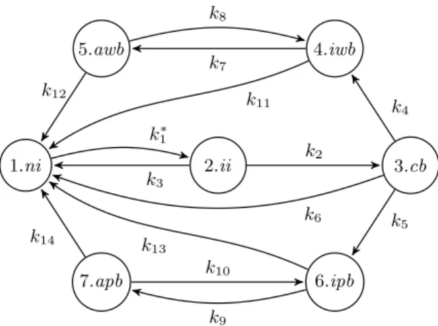
1.ni 2.ii 3.cb 4.iwb 6.ipb 5.awb 7.apb k∗1 k2 k3 k6 k4 k5 k11 k7 k13 k9 k12 k8 k14 k10
Fig. 2: Possible states of a computer in the network. The shorthand names
are defined as follows: ni=NotInfected, ii=InitialInfection, cb=ConnectedBot,
iwb=InactiveWorkingBot, awb=ActiveWorkingBot, ipb=InactivePropagationBot, and
apb=ActivePropagationBot.
4
Mean-field Analysis of a Bot-net
In this section we discuss the applicability of the mean-field method to modeling peer-to-peer botnet, similarly to [31] . In Section 4.1 we discuss the character-istics of the botnet, which are important for modeling. Section 4.2 describes the mean-field model of the botnet spread. The performance evaluation results are presented in Section 4.3, together with an example of wider usability of the mean-field model.
4.1 Description of the system
Let us describe the steps each computer goes through during the botnet spread. The computer which is inNotInfected state (S1) enters theInitialInfection(S2)
state with rate k1∗. Then, it connects to the other bots in the botnet, going to
ConnectedBot state (S3), and it downloads the program containing the malware
with rate k2. If the computer, for some reason, is not able to download the
malware, it returns to the stateNotInfected with ratek3.
After downloading the malware, the computer joins the botnet either as In-activeWorkingBot (S4) or asInactivePropagationBot (S6) with ratesk4andk5,
respectively. If downloading the malware is not possible, for example, because the connection has failed, the computer moves back to the NotInfected state with rate k6. Once the bot becomes either an InactiveWorkingBot or an In-activePropagationBot it never switches between the Working- or Propagation -classes. In order not to be detected, the bot is inactive most of the time and it only becomes active for a very short period of time. Transitions from Inactive-PropagationBot toActivePropagationBot(S7) and back occur with ratesk9and
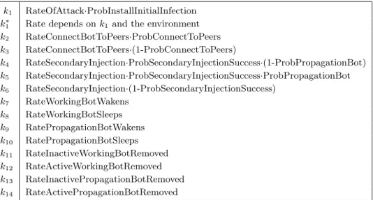
k1 RateOfAttack·ProbInstallInitialInfection
k1∗ Rate depends onk1 and the environment
k2 RateConnectBotToPeers·ProbConnectToPeers
k3 RateConnectBotToPeers·(1-ProbConnectToPeers)
k4 RateSecondaryInjection·ProbSecondaryInjectionSuccess·(1-ProbPropagationBot)
k5 RateSecondaryInjection·ProbSecondaryInjectionSuccess·ProbPropagationBot
k6 RateSecondaryInjection·(1-ProbSecondaryInjectionSuccess) k7 RateWorkingBotWakens k8 RateWorkingBotSleeps k9 RatePropagationBotWakens k10 RatePropagationBotSleeps k11 RateInactiveWorkingBotRemoved k12 RateActiveWorkingBotRemoved k13 RateInactivePropagationBotRemoved k14 RateActivePropagationBotRemoved
Table 1: Transition rates for a single computer.
k10, respectively. The transition rates for moving from InactiveWorkingBot to ActiveWorkingBot (S5) and back are denoted k7 andk8, respectively.
The computer can recover from its infection, e.g., if an anti-malware soft-ware discovers the virus, or if the computer is physically disconnected from the network. In these cases, it leaves theInactivePropagationBot or the Active-PropagationBot state and moves to the NotInfected state with rates k13, k14,
respectively. The same holds for the working bots: the transition rates from
InactiveWorkingBot andActiveWorkingBot arek11,k12, respectively.
The model we construct considers several computers in a network, each of them being in one of the above mentioned statesS1, .., S7, depicted also in
Fig-ure 2. The rates of transitions between states may depend on several factors, e.g., probability of a successful connection between initially infected computer and another infected computer, while moving from the stateInitialInfection to the
ConnectedBot state; or the probability of ConnectedBot to become Porking or
Propagationbot, respectively. Table 1 provides the description of the transition rates for one computer model, while numerical values are given in Table 2. Rates
k2. . . k14 are constant for each computer, while rate k∗1 to move from the Not-Infected state (S1) to the InitialInfection state (S2) is not constant. This rate
depends on k1 and on the number of computers in the ActivePropagationBot
state, which are responsible of spreading the malware.
4.2 Mean-field Model
We study the spread of the botnet in a network of N computers by using the mean-field approximation method for finding the (average) deterministic dy-namics of the system. The mean-field model captures the number of objects in a particular state, rather than considering the state of each single object. The mean-field state vectorX=hX1, X2, . . . X7icounts how many computers are in
We first construct the rate matrix, which collects the rates with which pos-sible transitions take place. Transition rates may depend on time as well as on the stateX(t) of the system. The rate matrixR(X(t)) of the model is given as:
R= 0 k∗1(X(t)) 0 0 0 0 0 k3 0 k2 0 0 0 0 k6 0 0 k4 0 k5 0 k11 0 0 0 k7 0 0 k12 0 0 k8 0 0 0 k13 0 0 0 0 0 k9 k14 0 0 0 0 k10 0 (1)
The|X|×|X|infinitesimal generator matrixQ(X(t)) is given as follows:Q(s1,s2)
is equal to the transition rateR(s1,s2) to move from the states1 to the state
s2 and Q(s,s) is equal to the reciprocal of the sum of all the rates in row s.
In a given example the only rate which depends on a state of the system is the infection rate k∗1(X(t)), which depends on the number of computers (bots) actively spreading infection. The total rate of infections produced by all bots that are in the active propagation state isk1·X7(t). These infections are spread
out randomly over all not-yet infected computers, whose number is denoted by
X1(t)5. Hence, the infection ratek∗1 perceived by each individual computer is
given by the ratio:
k∗1(X(t)) = k1·X7(t)
X1(t)
. (2)
which entails thatQsatisfies density dependence, as given in Definition 4. One we have constructed the infinitesimal generator matrixQ, we can use it to construct the set of Ordinary Differential Equations whose solution represents the average dynamics of the system. In particular, the drift matrixF is exactly the matrixQ. The state vector on the continuous state space isx=hx1, . . . , x7i.
Therefore, the initial value problem we study is defined as follows:
dx(t)
dt =x(t)Q(x(t)), with initial conditionx(0). (3)
The system of equations we obtain is:
˙ x1(t) = k3x2(t) +k6x3(t) +k11x4(t) +k12x5(t) +k13x6(t) + (k14−k1)x7(t) ˙ x2(t) = −(k2+k3)x2(t) +k1x7(t) ˙ x3(t) = k2x2(t)−(k4+k5+k6)x3(t) ˙ x4(t) = k4x3(t)−(k7+k11)x4(t) +k8x5(t) ˙ x5(t) = k7x4(t)−(k8+k12)x5(t) ˙ x6(t) = k5x3(t)−(k9+k13)x6(t) +k10x7(t) ˙ x7(t) = k9x6(t)−(k10+k14)x7(t) (4)
5 In the considered example the propagation bots are “smart” enough to spread
Experiments
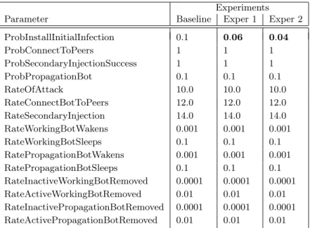
Parameter Baseline Exper 1 Exper 2
ProbInstallInitialInfection 0.1 0.06 0.04 ProbConnectToPeers 1 1 1 ProbSecondaryInjectionSuccess 1 1 1 ProbPropagationBot 0.1 0.1 0.1 RateOfAttack 10.0 10.0 10.0 RateConnectBotToPeers 12.0 12.0 12.0 RateSecondaryInjection 14.0 14.0 14.0 RateWorkingBotWakens 0.001 0.001 0.001 RateWorkingBotSleeps 0.1 0.1 0.1 RatePropagationBotWakens 0.001 0.001 0.001 RatePropagationBotSleeps 0.1 0.1 0.1 RateInactiveWorkingBotRemoved 0.0001 0.0001 0.0001 RateActiveWorkingBotRemoved 0.01 0.01 0.01 RateInactivePropagationBotRemoved 0.0001 0.0001 0.0001 RateActivePropagationBotRemoved 0.01 0.01 0.01
Table 2: Setup for the three experiments. Bold indicates differences w.r.t. baseline. The equations can be solved analytically, however the closed forms are impracti-cally large. We used Wolfram Mathematica [45] to obtain the analytical solution.
4.3 Results
In this section we discuss the mean-field results in detail and compare them to the simulation results, the chosen parameters for all these experiments are given in Table 2. We essentially experimented considering different infection rates, denoting possible user behaviors, and their impact on the system behavior.
The simulation of the model was done using the Moebius tool [19] as in [44]. Each experiment covered one week of simulated time. Each experiment was repli-cated 1000 times; the mean values and 95% confidence intervals of the measures of interest are shown. The initial conditions for each experiment are as follows: 200 computers are located in the placeActivePropagationBots.
We use Mathematica [45] to obtain solutions for the set (4) of differential equations coupled with the transition rates from Table 2. Given an overall popu-lation ofN = 107, the fraction of computers in the stateNotInfectedis initialized
as x1(0) = (N−200)/N, the fraction of computers in the state ActivePropaga-tionBot is initialized as x7(0) = 200/N, and the fractions of computers in all
other states are initialized as zero.
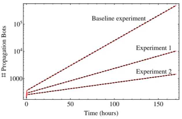
Figure 3 shows the number of the propagation bots along time. The number of propagation bots (both active and inactive) has been taken as measure of interest since they actively infect “healthy” computers. A logarithmic scale has been chosen for the number of propagation bots, in order to better visualize the exponential growth. The figure depicts the mean-field results of the Baseline
ex-Baseline experiment Experiment 1 Experiment 2 0 50 100 150 1000 104 105 TimeHhoursL ð Propagation Bots
Fig. 3: Number of propagation bots over time in the Baseline experiment and exper-iments 1 ad 2 obtained from mean-field approximation together with the confidence intervals obtained from the simulation.
Experiment Simulation Mean-field
Baseline 5 d 3 h 25 min 1 sec
Exp. 1 9 h 51 min 1 sec
Exp. 2 5 h 37 min 1 sec
Table 3: Time spent on simulation and mean-field approximation.
periment together with the 95% confidence intervals of the Moebius simulation. As can be seen, the mean-field results are very accurate in this case, since they lie mostly within the confidence intervals, even though the confidence intervals are very narrow.
To investigate how a reduced infection spread would influence the growth of botnets, Experiments 1 and 2 were done in [44]. The “user factor” ( ProbInstal-Infection) is reduced to 60% and 40%, respectively, as compared to the Baseline experiment to represent a lower probability of, e.g., opening infected files. The results are, together with those from the Baseline experiment, presented in Fig-ure 3. For both experiments, the results obtained with the mean-field model are very accurate and lie well within the confidence intervals most of the time.
One of the advantages of the mean-field method is that the time, needed for obtaining the means of the model is much smaller than the time, needed for the simulation (as shown in Table 3). The timings were obtained on a i7 processor with 3 GB RAM and 4 hyper-threading cores. The baseline experiment took 5 days 3 hours and 25 minutes, while the mean-field analysis was completed in one second. The difference between the simulation time for the different experiments is due to the dependency of the rates on a number of computers in ActiveProp-agationBots state. In the Baseline experiment the number of these computers is large, hence, the rate of infection becomes very large and more time is needed to simulate the resulting large number of events. The time spent on the simulation of the experiments with a lower number of computers involved is reasonably smaller; however the mean-field approximation is still much faster in all cases.
We do not provide all the experiments from [44] and [31] since they lie out of the scope of interest of this tutorial. Note, however, that the accuracy of the results and the speed of calculation hold for all the experiments, provided in the papers, mentioned above.
The speed of the mean-field results calculation allows us to use the mean field method to address problems which are not feasible using simulation: (i) we study the dependence of the botnet spread on two parameters, while the previous results are only functions of time for a given set of parameter values, (ii) and we study the behavior of the botnet in the presence of cost constraints. The purpose of the following is to show the difference between the simulation and the mean-field capabilities, and, at the same time, to show the advantages of the fast analysis.
We calculate the number of propagation bots as a function of k13 and k14
(see Figure 4). As one can see, there is no considerable difference in a relative increase of one or the other parameter. It is known that inactive computers are much harder to detect (increasingk13is more difficult), therefore the above
results might be helpful for the antivirus software developers to find the better strategy for botnet removal.
Next, we introduce a cost concept to analyze the economical side of an infec-tion. Two types of costs are considered: (i) the cost of a computer being infected, for example due to the loss of information or productivity, and (ii) the cost of more frequent checking with antivirus software. On one hand the number of infected computers, and hence their cost grows if computers are not frequently checked. On the other hand, if computers are checked too often the botnet is not growing, but running the antivirus software becomes very expensive. We analyze this trade-off in more detail in the following. We calculate the cumulative cost betweent0 andt1 as follows:
C(t0, t1, RR, D1, D2) = Rt1
t0 (D1·IC(t, RR) +D2·RR·AC )dt (5) whereRRis the change in removal ratesk11, ..., k14with respect to the rates in
the baseline experiment, i.e. k11 =RR·k11,baseline (similarly fork12, k13, k14);
D1 is the cost of infection; IC(t, RR) is the number of infected computers for
a given RR, at time t, including active and inactive working and propagation bots; D2 is the cost of one computer being checked, which probably is much
lower than the cost of infection (D1); AC is the number of the computers in the network. We calculate the cumulative cost of the system performance for three days. ForRR from the interval [0.001; 5] we calculate the cost as a function of time for given D1 and D2. Results are depicted in Figure 5 and, one can see,
that the cost grows exponentially with time and almost linearly with decreasing
RRif the computers are not checked frequently (for the RR between 0 and 1). However, if antimalware software is used too often (RR above 2), the cost grows linearly withRR.
We see that the mean-field method can be easily used for finding the removal rates which minimize the cost at a given moment of time. It can help network managers with careful decision-making, based on the situation at hand. Even
Fig. 4: Number of propagation bots for (k13, k14)∈[8·10−5; 10−3]×[8·10−3; 10−1]
at time T = 3days, all other parameters
are the same as for baseline experiment (see Table 2).
Fig. 5: Cost of the system performance for
D1= 0.01, D2= 4·10−5.
though not all parameters might be known in reality, such analysis can help to obtain a better understanding of the characteristics of botnet spread.
In this section the basic mean-field example was described together with the possible extensive use of the mean-field model. An example of using mean-field approximation for more sophisticated systems is given in the next sections.
5
Spatial Mean Field Models
Early use of the mean-field analysis technique stems from the fields of physics (e.g. when studying gas dynamics) and systems biology (e.g. studying how con-centrations of reactants behave in a solution). In those domains, the spatial dis-tribution of particles/molecules across the system is not described in the model. Indeed, they assume that particles/molecules are uniformly spread across the space, thus ignoring the effect locations have on the overall dynamics. Systems where this assumption is realistic are often referred to ashomogeneous, in physics, andwell-stirred, in chemistry. In practice, this assumption implies that a single rate can be assigned for each type of particle-to-particle interaction, regardless of the spatial structure, and the interactions have the same probability to take place at any location.
In this section we focus on the appropriateness of this abstraction in the mean-field method, particularly in the context of modelling computer and com-munication networks. Depending on the nature of a given system, ignoring lo-cations might be a suitable simplifying step. In our previous example, where we studied the spread of a virus in a network, the decision was made not to include the location of the computers. This led to a state vectorξ which only counted how many agents are in each of the states ni,ii,cb,iwb,awb,ipband apband the transition rate functions did not depend on distribution of computers across different geographical locations. Nevertheless, there exist systems whose dynam-ics and emergent behaviour are in fact, significantly dependent on locations. For such systems, if the model does not take into account such a spatial aspect,
the system behaviour may not be captured effectively. In such cases, the model should include an appropriate notion of agent location.
In this section, we consider an example of a large-scale peer-to-peer gossip network [14] where the emergent behaviour of the system significantly depends on locations. We describe, for this example, how the mean-field equations are constructed in a way that they also capture the effect that locations have on the system behaviour.
A second extension we present in this section concerns the application of the deterministic approximation theorem touncountabledomains. In Section 4 we il-lustrated an application of mean-field approximation to a finite-domain CTMCs. However, Kurts Theorem [33], as well as derived theorems (see Section 3), can be applied to Markov chains on countable domains [38]. The example considered in this section falls outside the scope of those results as it is applied on a Markov stochastic process on acontinuousdomain. Indeed, individuals (that is, taxis in this case) hold information concerning their location, that ranges on a finite set, and on the age of certain information they carry, that ranges on positive, real numbers. We will not address the technicalities related to this extension, but we point out this result, which in [14] is proved for the specific model considered and, in general, can not be obtained in a straightforward way. The uninterested reader can simply ignore this aspect and focus on the modelling of space.
5.1 The Age of Gossip
We consider the example from [14], which models a peer-to-peer communication network where two types of agent are present: some can move through different locations (mobile) and some others are stationary (base stations). The base stations transmit fresh updates on a piece of data through radio waves and these updates are received by the mobile agents. The data is time-stamped. The age of a piece of data on an agent is defined to be the time elapsed since last emission from a base station. Theage of data received by an agent from a base station iszero. Agents are capable of radio communication between themselves. If two mobile agents get close enough, the agent who has the most recent version of data transmits the data to the other agent. The data exchange between two entities (a mobile agent receiving data from a base station or a mobile agent communicating with another mobile agent) takes place when the entities get close enough to establish a radio connection.
The system consists of a finite number oflocationsthrough which the agents can move. Each mobile agent can only be in one location at any time. The base stations in location c can establish radio communication only with agents who are in the same location. The data exchange between two mobile agents can take place either when the communicating agents both belong to the same location or when they are in two different locations. The latter type of communication captures, for example, the situation when two nodes from different locations are at the borders of adjacent locations and exchange data. We are interested into studying how, in each location, the age distribution of agents evolves over time.
A Formal Description. Let L = {1,2, . . . C} denote the set of locations
and assume that there are N mobile agents who are moving across these
lo-cations. Let us define the variable Xi to represent the age of the ith node
and ci to represent the location of node i. Hence, the state vector is ξ =
hX1, X2, . . . XN, c1, c2. . . cNi, Xi ∈ R≥0, and ci ∈L. We define the transitions
and the rate function associated with each transition:
1. Mobility.A node can move from a locationcto another locationc0(c, c0∈L,
c6=c0) with rateρ
c,c0. When there areNc nodes in locationc, the total rate
at which nodes from locationcmove to locationc0 isNc×ρc,c0.
2. Contact with base.An agent i with age Xi in location c ∈ L can
com-municate with a base station in locationcand get fresh information. As the result of this data exchange,Xi becomes zero. For each locationca
param-eterµc describes the rate at which a node in locationc can get information
directly from base stations. If there is no base station inc, thenµc= 0.
3. Opportunistic contact within location.An agenti in location c com-municates with another agent in the same location with rate 2ηc/(N−1).
For each locationc, there exists a parameterηc, given by the modeller. This
parameter is not dependent on the population of agents in that location. Even when two locations have the same population level, the rate at which the agents interact in those locations may not be the same. Indeed, the topo-logical structure ofc might encourage the agents to meet more frequently thanc0 and consequently, one will observe a higher interaction rate incthan inc0. The total interaction rate in locationc is a function of both the popu-lation in that location (Nc) andηc. Defining such a constant will particularly
be useful when the modeller possesses real data about the execution of the system and wants to find parameters fitting the given data. If there areNc
nodes in locationc, the total rate at which two nodes communicate is:
Nc 2 × 2ηc (N−1) = (Nc)×(Nc−1) N−1 ηc.
This total rate includes the interaction of a node with nodes of any age. 4. Opportunistic contact across locations.A mobile agent in locationccan
communicate with a mobile agent from a neighbouring locationc0, (c6=c0). This transition happens with rate 2βc,c0/(N−1). For eachcandc0, (c6=c0),
βc,c0 describes a constant which affects the rate at which the agents in c
communicate with the agents inc0. The communication takes place only if there is at least one agent inc and one inc0.
State Space Representation - Choices. The location of each agent is one of its properties. For agent i, its location is in L = {1,2, . . . C}. If we con-sider only this property of the agents, then the state vector would be ξ0(t) = hξ10(t), ξ20(t), . . . ξC0 (t)i where for each location i, ξ0i represents the population count at that location. Such population counts change over the course of time as the agents move between locations.
Let us assume that we use the state vector ξ0 to model the peer-to-peer network and study how the system evolves. In the mean-field method, for each population count one differential equation is constructed. Therefore, givenξ0, the system of differential equation will haveCequations. The state space representa-tionξ0 and the corresponding set of differential equations capture the evolution of agents only with respect to their locations. Using such a state representation, the other important property of the agents, i.e. their ages, is ignored.
Let us now consider how to model the other property of the agents, their age. The age of an agent can take values inR≥0. An agent has age zero if it has
just had a communication with one of the base stations. The state of the system at timetcan be characterized by a continuous distributionξ00(z, t) with domain
R≥0. ξ00(j, t) captures how many agents have age (around) j at time t. Using
the state representation ξ00(j, t), one can construct a set of partial differential equations, over the dimensions j and t, which captures how the agents evolve in terms of their age distribution as the time elapses. The shortcoming of this analysis is that the location of the agents, which has significant effect on how the age distribution evolves, is completely ignored.
In order to faithfully capture the dynamics of the considered system, a com-bination of both state representations ξ0 and ξ00 is needed, to consider both properties of the agents: their locations and their ages.
Mean Field State Space Representation. Consider a location c. For the
ith agent, who has ageX
i, let us define the distribution δXi which is a Dirac
mass atXi. At a timet, the age distribution of agents in locationc acrossR≥0
is characterized byMN c (t): McN(t) = N X i=1 1{ci=c}δXN i (t).
which is a continuous distribution denoting the number of agents who have age (around)z at locationc and timet. The vector of continuous distributions
MN(t) =hM1N(·, t), M2N(·, t), . . . , MCN(·, t)i is defined in term d of the distributions MN
c (z, t), for each location c ∈ L,
discussed above. This vector captures both location and age of an agent and is used, in the rest of this section, for mean-field analysis.
5.2 Mean-Field Limit Behaviour
In order to find the deterministic limit behaviour of the system, we first focus on the dynamics of the population moving across locations.
Mobility of the Agents. Let U(t) = hU1(t), U2(t), . . . , UC(t)i be a vector
such that Uc(t) denotes the number of agents in location c at timet. The
¯ UN(t) = U(t) N =hU¯ N 0 (t),U¯ N 1 (t), . . . ,U¯ N C(t)i.
indicating the fraction of agents per location, at timet. Assume that, forN → ∞, the sequence ¯UNc (0) converges to a unique limit (Definition 3):
lim N→∞ ¯ UN(0) = lim N→∞ U(0) N = U1(0) N , U2(0) N , . . . , UC(0) N = ¯ u0 1,¯u02, . . .u¯0C =¯u0
Following [14], since convergence of initial occupancy measure holds and since constant mobility rates imply density dependence, we can apply Kurtz Theo-rem [34] (TheoTheo-rem 1), and prove thatat any time t >0, forN → ∞, the pro-cesseU¯N(t) converges to a deterministic processu¯(t) = hu¯1(t),u¯2(t), . . .¯uC(t)i
where ¯uc(t)c∈L is the solution of the following initial value problem:
∀c∈L, ∂ ¯uc(t) ∂t = X c06=c ρc0,cu¯c0 − X c06=c ρc,c0 ¯uc (6) ∀c∈L, ¯uc(0) = ¯u0c
The first term on the right hand side of Equation (6) indicates the increase of ¯
uc due to agents coming from adjacent locations. Similarly, the second term
indicates the decrease of ¯uc due to agents going towards adjacent locations.
According to [14], by the Cauchy-Lipschitz theorem, for any initial condition ¯
u0=h¯u0
cic∈L, the above initial value problem admits a unique solution.uc(t|¯u0)
denotes the deterministic value of the location occupancy measure at timetgiven the initial condition ¯u0. In [14] the system behavior is studied at stationary
mobility regime. For this purpose one can use the fixed point method: ∀c∈L, ∂ ¯uc(t) ∂t = 0 ⇒ (7) ∀c∈L,u˜c X c06=c ρc0,cuc0 = X c06=c ρc,c0 u˜c , X c∈C ˜ uc= 1
The solution of the above equation, ˜u, shows how the agents are spread across the locations when the system reaches its equilibrium.
Propagation of Information - Age Distribution. Consider the state vector
M. For an agent populationNand a timet, let us define the system’s occupancy measure as a vectorM¯N of continuous distributions:
¯
MN(t) =M N(t)
N =hM¯1(·, t),M¯2(·, t), . . . ,M¯C(·, t)i
For locationc, ¯MN
c (z, t) denotes thedensity of agents in locationcwith agezat
timet. For ¯MN
c (t), one can define its cumulative distribution functionFcN(z, t):
∀c∈L, FcN(z, t) =McN(t)[0 :t] =
Z z 0
¯
For location c, age z and timet,FN
c (z, t) tells us what proportion of the total
population, at timet, is in class c with the ageless than or equal to z.
We assume that, for N → ∞, similarly to U¯N(0) → ¯u0, the vector of the occupancy measuresM¯N(0) converges to a unique limit vectorm¯0:
lim
N→∞
¯
MN(0) =m¯0
This means that for each location, the corresponding occupancy measure ¯MNc (0)
converges to a unique limit distribution m¯0c (Definition 3):
∀c∈L , lim N→∞ ¯ MNc (0) = ¯m 0 c
As a consequence, at any given timet >0 and for allc∈L, whenN gets large, the density ¯MNc (t) converges to ¯mc(t), where ¯mc(t) is the solution of the following
partial differential equation. In the following equation, ¯uc(t) is the solution of
Equation (6), the population of agents in locationc at timet. ¯ mc(0, t) =µc×u¯c(t) (8) ∂m¯c(z, t) ∂t =− ∂m¯c(z, t) ∂z −µc×m¯c(z, t) +X c06=c ρc0,cm¯c0(z, t)− X c06=c ρc,c0 m¯c(z, t) +2ηc[(+1)×(uc(t)−Fc(z, t))·m¯c(z, t) + (−1)×m¯c(z, t)·Fc(z, t)] +X c06=c 2βc,c0(+1)×(uc(t)−Fc(z, t))·m¯c0(z, t) + (−1)×m¯c(z, t)·Fc0(z,t)
The formal proof of convergence is presented in [14]. However, here we use a more intuitive description, also presented in [14], to understand how the equations above are constructed.
Equation (8) can be formed by considering how much each ¯mc(z, t)c∈Cchanges
in a small period of time∂t(the left hand side). Consider locationc. During∂t, agents with agez, which have been accounted for by ¯mc(z, t), will become older.
Consequently, such agents need to be removed from ¯mc(z, t). On the other hand,
agents who currently have the age z− 4z will become older and therefore, the density ¯mc(z− 4z, t) will be added to ¯mc(z, t). Hence, the rate of change of
mc(z, t) caused only byaging is:
lim 4z→0 |m¯c(z− 4z, t)−m¯c(z, t)| 4z = ∂m¯c(z, t) ∂z
This is captured by the first term on the right hand side of Equation (8). The second term reflects the communication of agents, accounted by ¯mc(z, t), with
one of the base stations in their same location. Communicating with one of the base stations reduces the agent’s age to zero and hence, such agents have to
be removed from ¯mc(z, t). If there are ¯mc(z, t) agents in location c, given that
the rate of communication with a base station in c is µc, then, in a period of
∂t, µc ×m¯c(z, t)×∂t of the agents will communicate with the base stations
and hence, have to be removed from ¯mc(z, t). The rate of the change is then
calculated asµc×m¯c(z, t).
The third expression shows the flow of agents into ¯mc(z, t) as a result of
agents with age z moving from neighbouring locationsc0 into c, (c6=c0). For a givencandc0, such movement decreases ¯mc0(z, t) and increases ¯mc(z, t).The flow
rate from ¯mc0(z, t)c0∈Linto location ¯mc(z, t) at time t isρc,c0m¯c0(z, t). Similarly,
the fourth term reflects the movement of some of the agents contained in ¯mc(z, t)
out ofcinto the adjacent locations. The flow rate is calculated similarly. The fifth term has two parts. The first, 2ηc×(uc(t)−Fc(z, t)).m¯c(z, t), shows
the rate of flow into ¯mc(z, t) because of agents with the age higher than z inc
communicating with agents who have agezin the same location. When an agent of age higher thanz communicates with an agent of agez, the age of the older one reduces toz. The total density of agents in locationcat timet is ¯uc(t) and
the density of agents whose age is less than or equal to zis Fc(z, t). Therefore,
the density of agents with age higher thanz in c is (uc(t)−Fc(z, t)). The rate
expression depends on the density of population of agents in c with age higher thanz, the density of agents incwith the agez and additionally, onηc.
The second part:−2ηc×( ¯mc(z, t))×Fc(z, t) shows the drift out of ¯mc(z, t) as a
result of agents with the agezinccommunicating with the agents of lower age in the same location. The interpretation of the sixth term is similar, the difference being that it captures the communications which take place between the agents who belong to two different locations c and c0 as opposed to a communication where two parties belong to the same location.
If we simplify the equation above and integrate overz, we obtain the following equation forFc(z, t): ∀c∈L: ∂ Fc(z, t) ∂t = −∂ Fc(z, t) ∂z + X c06=c ρc0,cFc0(z, t) − X c06=c ρc,c0 Fc(z, t) (9) + (uc(t|d)−Fc(z, t))(2ηcFc(z, t) +µc) + (uc(t|d)−Fc(z, t)) X c06=c 2βc,c0Fc0(z, t) ∀c∈L,∀t≥0 :Fc(0, t) = 0 ∀c∈L,∀z≥0 :Fc(z,0) =Fc(z)
Note that this model relies on the assumption that the agents’ movements do not depend on the information propagation scheme. Therefore, the set of ODEs (6) which capture the evolution of the location occupancy measure can be constructed and solved independently.
5.3 Solution of the Equations
Let us now describe how the solution of Equation (9) is obtained for the case
where there is only one location in the system and assuming that when the
system starts att= 0, every agent has age zero.
The solution is found by introducing a change of variables. Let us define the spaceA={(x, y)∈R×R|x≥0, x+y≥0}. The functionG(x, y) :A→[0,1] is
defined asG(x, y) =F(x, x+y). Therefore, in order to knowF(z, t) it is enough to calculateG(z, t−z). For a functionGdefined as follows:
∂G(x, y) ∂x = ∂F(z, t) ∂z (x,x+y)+ ∂F(z, t) ∂t (x,x+y) .
Rearranging the terms in Equation (9), we obtain:
∂G(x, y)
∂x = (1−G(x, y))(2η G(x, y) +µ) for G(0, y) = 0 (10)
The assumption that at timet= 0, no gossip exists in the network leads to the conclusion that at any given time z < t and y = t−z > 0. For an arbitrary value ofy∈R+, let us definegy:x7→G(x, y). Therefore:
∂gy(x)
∂x = (1−gy(x))(2ηgy(x) +µ) for gy(0) = 0
By Cauchy-Lipschitz Theorem, this equation has a solution. Once the value of
gy(x) for a givenxis found, the correspondingF(z, t) can be easily calculated.
Single Location - Analytical Solution. In this case, the ODE can analyti-cally be solved and leads to the following solution:
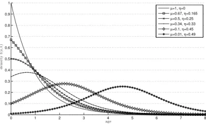
F(z, t) = 1− 2η+µ 2η+µe(µ+2η)z if z≤t 1− 2η+µ 2η+21ηF−(Fz(−zt,−0)+t,0)µe(µ+2η)t if z > t (11)
Consider that above, we illustrated the reasoning behind the first case of the solution (when z ≤ t). The second case (z > t), corresponds to the situation where in the initial configuration of the system some agents have age greater than zero. Therefore, at some time t, it is possible that some of the agents in the system have ages higher than t. The proportion of the agents who at time
t have age z > tdepends on the proportion of the agents who had age at least (z−t) in the system initial configuration.
Performance Evaluation of Peer-to-Peer Dynamics. In terms of perfor-mance, a well designed peer-to-peer opportunistic network should guarantee
![Fig. 4: Number of propagation bots for (k 13 , k 14 ) ∈ [8 · 10 −5 ; 10 −3 ] × [8 · 10 −3 ; 10 −1 ] at time T = 3days, all other parameters are the same as for baseline experiment (see Table 2).](https://thumb-us.123doks.com/thumbv2/123dok_us/434300.2550155/21.918.208.716.192.338/fig-number-propagation-bots-parameters-baseline-experiment-table.webp)
![Fig. 8: The green solid line shows P rob M l (s 1 , not infected U [0,1] infected, t 0 , t).](https://thumb-us.123doks.com/thumbv2/123dok_us/434300.2550155/42.918.220.721.357.531/fig-green-solid-line-shows-rob-infected-infected.webp)