A Tutorial on Machine Learning for Failure Management in Optical Networks

04 August 2020

Repository ISTITUZIONALE

A Tutorial on Machine Learning for Failure Management in Optical Networks / Musumeci, F.; Rottondi, C.; Corani, G.; Shahkarami, S.; Cugini, F.; Tornatore, M.. In: JOURNAL OF LIGHTWAVE TECHNOLOGY. ISSN 07338724. -ELETTRONICO. - 37:16(2019), pp. 4125-4139.

Original

A Tutorial on Machine Learning for Failure Management in Optical Networks

ieee Publisher: Published DOI:10.1109/JLT.2019.2922586 Terms of use: openAccess Publisher copyright

copyright 20xx IEEE. Personal use of this material is permitted. Permission from IEEE must be obtained for all other uses, in any current or future media, including reprinting/republishing this material for advertising or promotional purposes, creating .

(Article begins on next page)

This article is made available under terms and conditions as specified in the corresponding bibliographic description in the repository

Availability:

This version is available at: 11583/2768632 since: 2019-11-25T15:26:17Z

1

A Tutorial on Machine Learning for Failure

Management in Optical Networks

Francesco Musumeci

, Cristina Rottondi

, Giorgio Corani

, Shahin Shahkarami

, Filippo Cugini

, and

Massimo Tornatore

_{Politecnico di Milano, Italy,}

_{Dalle Molle Institute for Artificial Intelligence (IDSIA)}

_{Consorzio Nazionale Interuniversitario per le Telecomunicazioni (CNIT)}

Abstract—Failure management plays a role of capital impor-tance in optical networks to avoid service disruptions and to satisfy customers’ service level agreements. Machine Learning (ML) promises to revolutionize the (mostly manual and human-driven) approaches in which failure management in optical networks has been traditionally managed, by introducing au-tomated methods for failure prediction, detection, localization and identification. This tutorial provides a gentle introduction to some ML techniques that have been recently applied in the field of optical-network failure management. It then introduces a taxonomy to classify failure-management tasks and discusses possible applications of ML for these failure management tasks. Finally, for a reader interested in more implementative details, we provide a step-by-step description of how to solve a representative example of a practical failure-management task.

Index Terms—Machine Learning; Failure Management.

I. INTRODUCTION

The importance of failure management in Optical Networks (ONs) is superior to any other network domain, as failures in ONs can induce service interruption to thousands, if not millions, of users. Consider, e.g., the case of the fiber cuts in Mediterranean Sea in 2008 that caused loss of 70% of Egypts connection to outside world and more than 50% of Indias connectivity on the westbound route [1]. Even in much less disruptive scenarios, the ability of an ON operator to quickly recover a failure is crucial to meet Service Level Agreements (SLAs) to its customers.

Despite its importance, ON Failure Management (ONFM) still often requires complex and time-consuming human in-tervention, and increased automation of failure recovery is a fundamental element in operators’ roadmaps for the years to come. A promising direction moves towards the utilization of advanced statistical/mathematical instruments of Machine Learning (ML) to automate the ONFM tasks.

The application of ML in ONFM is challenging for several reasons: i) the quantity of data that can be monitored in modern ONs is enormous, and scalable “analytics” techniques must be considered [2], [3]; ii) several kinds of failures (not only fiber cuts, but also equipment malfunctioning and misconfiguration, network ageing, etc.) can affect an ON connection (lightpath); iii) failure management in ONs tends to be more challenging than in other domains (e.g., at IP-level) as ONFM is inherently cross-layer, i.e., it must jointly consider physical-layer and network-layer aspects. To deal with this multifaceted problem, effective ONFM shall be constituted

by several sequential tasks, in each of which ML can play an important role towards automation. To provide a complete introduction to the topic, in this tutorial:

• we motivate the usage of ML in ONFM and provide a

gentle introduction to the main ML principles and cat-egories of ML techniques, focusing on those algorithms that have been already used in previous works,

• we categorize the various phases of ONFM as opti-cal performance monitoring, failure prediction and early detection, failure detection, failure localization, failure identification and failure magnitude estimation,

• for each of category, we provide a description and some examples, and we discuss which ML methodologies can be applied for solving them,

• we finally provide a step-by-step description of how to practically solve a representative ONFM procedure, breaking down the various steps (collection and prepara-tion of data, algorithm design, performance analysis). While surveys summarizing existing proposals for ML ap-plications in ONs have recently appeared [4], [5], this paper adopts a more tutorial style and is intended to offer a specific introduction to the application of ML methodologies for failure management. We also refer the readers to other two recent tutorials (Refs. [6] and [7]) that comprehensively cover ML applications in the field of optical networking and optical communications, respectively, but do not provide the same focus on failure management.

The paper is structured as follows. Section II elaborates on the main motivations for the application of ML in ONFM. Section III provides basic notions on the most-promising ML algorithms for ONFM. Section IV presents our taxonomy for ONFM tasks and discusses, for each task, some proposed ML solution. In Section V we describe, step-by-step, how a comprehensive ML-based solution, covering the task described in Section IV, can be structured. Finally, section VI discusses some future directions and current standardization activities.

II. MOTIVATION

A. Why ML?

Why ML, a very well-investigated methodological area (its first applications date back to the 60s), has been attracting attention for ONFM only in recent years? While the answer in not necessarily purely technical, we can identify some recent technological trends in ONs that are paving the way

(a) supervised learning for fault identification

(b) unsupervised learning for fault detection and localization Fig. 1: Supervised vs. unsupervised learning in ONFM

towards effective ML applications:

i) Modern optical equipment (transceivers, reconfigurable optical add-drop multiplexers, amplifiers) are now installed with built-in monitoring capabilities [8], and they are capable to generate a large amount of data, which can be leveraged to automate ONFM using ML.

ii) The large amount of data collected through such monitors can now be collected and elaborated in (at least logically) centralized locations thanks to new advanced control/management solutions, as network telemetry, SDN [9] and/or orchestration frameworks [10].

iii) Network intelligence (computing capabilities) can now be placed virtually everywhere (e.g., leveraging Network Function Virtualization and/or Mobile Edge Computing).

B. How does ML work?

ML algorithms aim at extracting knowledge from data, based on some characterizing inputs, often referred to as attributes or features. Depending on the available data and on the objective of the model to be developed, ML techniques can be classified at high level in the following categories:

• Supervised ML algorithms are given as input labelled data, i.e., there is a set of historical training data

sam-ples containing both the input values (features) and the corresponding output, namely the labels. Such labels can be either numerical values in a continuous range or discrete/categorical values. In these two cases, supervised learning takes the form of a regression or classification problem, respectively. Consider e.g., the case in Fig. 1a, where the objective is to identify the nature of a fault based on a series of Bit Error Rate (BER) measurements collected at the receiving nodes of various lightpaths during past fault events. Each ligthpath is characterized by a set of features including route, modulation format, wavelength used for transmission and observed BER trend. The ML algorithm learns how to associate such features to the correct failure cause (e.g., an amplifier malfunctioning or a fiber bending).

• In unsupervised ML algorithms, data is not labelled. Now, given the available/collected data, the objective is to identify if there are useful similarities among data (this is usually referred as clustering) or if there are notable exceptions in the data set (this is usually referred to as “anomaly detection”). An intuitive application is shown in Fig.1b, where the objective of applying ML is to detect a failure based on historical BER measurements. After collecting enough data representing faulty and faultless lightpaths, the algorithm learns to discriminate where a fault is occurring (in this case on the path A-B-C-D). After detection, failure localization can also be performed by correlating the faulty and faultless routes: since paths A-B-C and A-D-C are faultless, the only possible location of the failure is on link B-D.

• Semi-supervised algorithms are hybrid of the previous two categories. These algorithms lend themselves to solve problems where only few data points are labelled and most of them are unlabelled (consider, those cases when labelled data are scarce or expensive, e.g., when labelled data require ad-hoc probing). Their application is particularly promising in the field of ONFM, as will be discussed later.

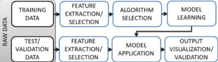
• Reinforcement learning (RL) is another area of machine learning in which an agent learns how to optimally behave (i.e., how to maximize the reward obtained over a certain time horizon) by interacting with the environment, receiv-ing a feedback after each action and updatreceiv-ing accordreceiv-ingly its knowledge. Yet, RL is not covered in this tutorial. In particular, in the case of supervised learning (see the first row of Fig. 2), the training phase includes the following steps:

• Raw training data are preprocessed to extract and select

features containing useful information for the regres-sion/classification task, i.e., showing statistical correlation with the output value/class.

• A suitable learning algorithm is selected. Several learn-ing algorithms, with different characteristics in terms of achievable accuracy, scalability and computational effort, have been proposed. In the next Section, we overview the most widely-adopted methods in ONFM.

• The chosen algorithm learns the regression/classification model, i.e., a mapping between the space of features and

3

Fig. 2: ML model construction and test workflow.

the associated outputs.

• To assess and improve the generalization properties of the algorithm developed at training phase, the ML algorithm can be applied over one or more validation datasets for which labels are also known, in order to fine-tune the algorithm parameters so as to avoid overfitting.

Once the training phase is concluded, the ML algorithm can be used over a test dataset containing new instances characterized by the same type of features of the training set (see second row of Fig. 2) and for which the corresponding outputs are known (i.e., they represent the ground truth), but are not used to perform the prediction. In general, in the test phase, the following steps are performed:

• Data are preprocessed for feature extraction and selection.

• The learned model is applied on the test dataset.

• The outputs provided by the algorithm are elaborated to be visualized and/or validated, by comparing the output of the model with the ground truth. To do this assessment, a wide set of metrics are used [11] (see Sec. III-G). On the other hand, in the case of unsupervised learning, the training phase is typically skipped and only the test phase is performed. However, note that in some cases, e.g., when performing anomaly-detection, a training phase can be present also in unsupervised algorithms.

Note that, in general, a ML algorithm is only part of a complex ONFM procedure, where the outputs of the ML algorithm (e.g., the output of a regression, a classification or a clustering algorithm) are exploited to perform further tasks. As an example, when considering ONFM, a ML algorithm can be developed and adopted to accurately identify the location of a failure within the network, i.e., to detect which network device is affected. After knowing the location of the failure, i.e., exploiting the output of the ML algorithm, the operator can take further actions (e.g., perform lightpath re-routing to bypass the failed network element), exploiting a different approach, not relying on ML (e.g., select the new path based on a precomputed list of alternative paths, or calculate the new path via other routing algorithms such as Dijkstra).

In summary, ML algorithms can become useful ONFM tools whenever an unknown relation between a set of input features (e.g., a set of alarms) and their corresponding output (e.g., if a certain element of the network must be substituted before it fails) must be identified. In the next section, we will outline the main ML algorithms used in ONFM.

III. BACKGROUND ONML TECHNIQUES FORFAILURE

MANAGEMENT

This section provides a high-level introduction to some ML techniques adopted in ONFM. We assume the reader to be already familiar with basic concepts such as decision trees, decision boundaries, and linear models for regression and classification. A gentle introduction to these topics is given in [12]. We also recommend the website [13], which provides tutorials on the most important ML algorithms.

A. Bagging and Random Forests

Bagging combines the predictions of different models into a single decision. In case of classification, it takes a vote: the prediction is the class predicted by most models. In the case of regression, the prediction is the average of the predictions of the different models. Bagging creates different models by training them on training data sets of the same size, which are obtained by modifying the original training data. In particular, some instances are randomly deleted while some others are randomly replicated; this resampling procedure is called bootstrap. Bagging creates via bootstrap B different training sets, with B being typically between 20 and 100. It then learns a different decision tree on each training set. Bagging is generally more accurate than a single decision tree. As we have seen, bagging generates an ensemble of classifiers by randomizing the original training data.

Differently from bagging, in Random forest (RF) the di-versity among the decision trees is increased by randomizing the feature choice at each node. In particular, the generation (“induction”) of decision trees requires selecting the best attribute to split on at each node; it is randomized by first choosing a random subset of attributes and then selecting the best among them. The RF algorithm usually achieves better accuracy than bagging, both in regression and in classification. An empirical comparison of different implementations of RF, with recommendations about default settings, is given by [14]. See [11, Chap.15] for a more detailed discussion of RF. In ONFM, RFs are applied for classification or regression tasks on time series constituted by samples of the monitored network parameters (e.g., BER, received power, etc.). Classification algorithms can be adopted, e.g., to distinguish between dif-ferent root causes of failures occurring in optical networks (failure identification). Instead, regression might be used to predict the future values of an observed network parameter based on a historical trend, so as to possibly raise alarms if the predicted value falls above/below given thresholds (failure prediction/early detection).

B. Bayesian Networks

A Bayesian Network (BN) is a compact representation of the joint distribution of multiple discrete variables. As-sume the involved discrete variables to be X, Y and Z; for simplicity, assume that each variable has cardinality k. The joint distribution P(X, Y, Z) assigns a probability to each possible combination of values of X, Y and Z; thus it requires storing k3 values. The size of an explicit rep-resentation of the joint distribution increases exponentially

Fig. 3: Example of a feed-forward NN with one hidden layer.

with the number of variables, and it is generally infeasible in real-world problems. Yet a BN efficiently represents the joint distribution of even thousands of variables by exploiting the conditional independences that exist among variables. IfXand

Y are independent given Z (i.e., X andY are conditionally independent), then the joint distribution can be factorized as

P(X, Y, Z) =P(Z)P(X|Z)P(Y|Z), which requires storing onlyk+ 2k2_{values. By exploiting conditional independences,}

a BN model sharply decreases the number of values that is needed to represent the joint distribution. Such independences can be either discovered from data or suggested from experts. The independences are then encoded into a directed acyclic graph. As BNs are typically learned on discrete data, they are typically adopted in classification tasks.

Once the network is learned, we can use it for making predictions, for instance computing the posterior probability for the remaining unobserved variables. This task is called inference. The most recent advances [15] allow learning and performing inference with Bayesian networks also in domains containing thousands of variables. See [16] for a book focused on modeling and inference with Bayesian networks; see [17] for a book which covers also other types of probabilistic graphical models. In the context of ONFM, BNs are applied for failure localization and root cause identification purposes, as they can capture correlations among thousands of interde-pendent networks components.

C. Artificial Neural Networks (ANN)

ANNs are a powerful tool for estimating unknown relations between features and outputs. An ANN is constituted by connected units (neurons), that are organized into layers (Fig. 3). Each neuron receives a set of values, one from each neuron of the previous layer. It computes a weighted sum of such values and it applies a non-linear transformation (sigmoid, Rectified linear unit (Relu), tanh, etc. [11]); the output of this function is then passed to the neurons of the next layer. Given a large enough number of neurons, the ANN model can approximate any function with arbitrary precision, thus constituting a universal approximator.

The estimation of the weights between the layers of an ANN is performed through the back-propagation algorithm. Finding the optimal architecture of the network (e.g., deciding how many neurons to place in each layer) has to be done via trial-and-error, paying attention to avoid overfitting (which implies poor predictions on instances which have are not present in

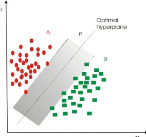
Fig. 4: The optimal hyperplane in a problem with two linearly separable classes. The margin of the optimal hyperplane is denoted by ρ. Picture taken from [21].

the training set). See [18, Chap.5] for a detailed discussion of training ANNs. Similarly to RF, ANN are mainly applied for failure prediction and identification in optical networks.

When ANNs are characterized by multiple hidden layers, they are referred to as Multi-Layer Perceptron (MLP). More-over, Deep Neural Networks (DNNs) constitute a particular form of MLP, where a high number of hidden layers are used. In general, adopting several hidden layers as happens in DNNs, increases the flexibility of the model, i.e., with DNNs more accurate models of complex input/output relations can be obtained. In simpler “shallow” ANNs, a hand-designed selection of input features is typically performed, so an accu-rate knowledge of the problem to be solved is required from a human expert. On the contrary, leveraging their multiple-hidden-layer hierarchy, DNNs enables an automatic learning of the importance of each input feature onto the output variables, thus simplifying the process of features selection [19].

For these reasons, DNNs excel in pattern recognition tasks [20], such as the extraction of features from images, the recog-nition of handwritten character recogrecog-nition, the processing of natural language. In the context of OFNM, the advantage of deep ANN is that they can be directly fed with raw measurements acquired from optical monitors, without need of feature extraction and selection procedures.

D. Support Vector Machines

Support vector machine (SVM) is a kernel methods [22]. Consider a bunch of points being classified into two classes by a single straight line as shown in Fig. 4. In this case, we can say that the two classes are separable. In an n-dimensional space, the optimal hyperplane is the one that represents the largest separation (margin) between the two classes. The instances that are closest to the maximum-margin hyperplane are called support vectors. SVMs identify such maximum-margin hyperplane and then use it as decision boundary. SVMs extend [12, Chap.7.2] the linear models (e.g., linear and logistic regression) as they learn the decision boundary in a high-dimensional space derived from the problem features.

5

A picture

Fig. 5: Relations between various regression and classification methods; picture taken from [26].

Note that, while data might be not separable in the original low-dimensional space of the attributes, they often become separable in an induced high-dimensional space. The function used to map an observation of the original attributes into a higher-dimensional space is called kernel function. Different kernel functions can be adopted with SVMs, such as, e.g., linear, polynomial or radial basis function kernels [11]. SVMs tend to be slower than other algorithms, but they often produce accurate classifiers. Like RFs and ANNs, SVMs are mainly applied in failure prediction and root cause identification. E. Gaussian Processes

The Gaussian process (GP) is a state-of-the-art approach for regression and classification; it can be seen as a Bayesian kernel method (Fig.5). A comprehensive book about GPs is [23] while many tutorials can be found in [24]. The optimiza-tion problems required for training SVMs and GPs are similar [23, Chap.6]; yet GP is a fully probabilistic model, hence its predictions are naturally accompanied by an assessment of their uncertainty. An interesting link can be drawn also with ANNs, as it has been shown that certain ANNs with one hidden layer are equivalent to a Gaussian process (but they lack the uncertainty assessment of the GP) [23, Chap. 7]. Another important advantage of the GP is that it can be trained without overfitting also on small data sets, unlike neural networks. On the other hand, the training procedure becomes heavy on very large data sets as its computational complexity increases cubically with the number of instances (sparse GPs algorithms have been developed recently to deal efficiently with big data [25]).

Given the probabilistic characterization of their output, GPs are particularly useful in ONFM whenever an assessment on the reliability of a classification/regression is required. As GPs return the probability that the instance belongs to one class,

depending on such outcome, different actions could then be triggered: for example, if the probability associated to class yes is99%, traffic rerouting would be applied, whereas if the probability is 51%, it could be better to wait for additional measurements before rerouting.

F. Network Kriging

Network Kriging (NK) is a mathematical framework that aims at individuating correlations among linear parameters. It was initially proposed in [27] to evaluate performance metrics of transmission paths spanning multiple links of a given network topology: NK considers path level measurements of a given performance metric, which is assumed to be a linear function of the values of the same metric measured along each link composing the path. As path monitoring in ONFM requires expensive equipment, NK is aimed at identifying a subset of deployed paths to be monitored: the choice of the monitored lighpaths is performed in such a way that deduction of path-level metrics of the non-monitored lightpaths is possible, based on the measurements collected on the monitored ones.

This technique finds direct application in ONFM, since optical monitors are typically placed at receiver nodes and thus provide path-level metrics, whereas link-level metrics (which are of more interest for, e.g., failure localization) can be directly obtained only at the price of installing additional monitoring devices at intermediate nodes. However, kriging works only under assumption that a linear relationship holds between link-level and path-level metrics. Such assumption typically does not hold for BER and Q-factor.

G. Cross-validation and statistical analysis of the results The classical method for estimating the accuracy of a ML algorithm is k-folds cross-validation (CV) [12, Chap. 5.4]. First, the data are split into k non-overlapping partitions (folds). At the i-th iteration, (k-1) folds are joined, forming the training setDi

tr; the remaining fold constitutes instead the test setDi

te. The classifier is learned onDtri and its accuracy is assessed onDi

te. Such training / test procedure is repeated several times, until each fold has been used once as test set. Sometimes, Leave One Out Cross Validation (LOOCV) is adopted. It corresponds to n-fold cross-validation, where

nis the number of instances in the dataset. Each instance in turn is left out, and the classifier is trained on all the remaining instances. See [12, Chap 5.4] for a more detailed discussion of the statistical properties of LOOCV.

The simplest measure of the quality of a classifiers is the accuracy, i.e., the proportion of instances which are correctly classified. Using cross-validation, the accuracy that will be achieved on future unseen data is estimated by averaging the accuracies obtained on the different test sets.

However, accuracy assumes that all errors are equally bad, while usually different types of error have different costs. For simplicity, assume the classification problem to be character-ized by two classes, thepositiveand thenegativeone. Assume the positive class to be the rarer outcome; for example the

failure in an ON. The negative class is instead the common outcome, hence the regular functioning of the network.

The most important goal is retrieve all the positive instances, i.e., all the failures; to this end we are willing to accept that some negative instances are labeled as positive, hence triggering some false alarms. A false positive (predicting a failure as regular) is hence a more severe error than a false negative (predicting a regular case to be a failure). In problems of this type, recall and precision [12, Chap. 5.7] are more relevant metrics than accuracy:

recall= number of positive cases predicted as positive

total number of positive cases precision= number of positive cases predicted as positive

number of positive predictions

Precision and recall are two contrasting objectives and dif-ferent algorithms give difdif-ferent trade-offs on these measures. The F-score (or F-measure) can be used to characterize the performance with a single measure:

F-score= 2· recall· precision

recall + precision

Sometimes it is necessary to choose between two or more algorithms, given their cross-validation results. Statistical anal-ysis of the cross-validation results is typically carried out through hypothesis testing. This procedure allows to ascertain whether the difference of performance between two algorithms can be due to random fluctuations, or if instead the difference between algorithms is statistically significant. See [28] for a discussion of the statistical tests used to compare cross-validated classifiers; see instead [29] for state-of-art Bayesian approaches to analyze cross-validation results.

IV. A TAXONOMY OFFAILUREMANAGEMENT IN

OPTICALNETWORKS

As depicted in Fig. 6, ONFM involves a variety of tasks that can be broadly categorized into 1) Proactive approachesand 2) Reactive approaches. At a high level, proactive approaches aim at prevention (i.e., avoidance) of service disruption, by anticipating failure occurrence, whereas reactive approaches respond to a failureafteror duringits occurrence, by quickly activatingrecoveryprocedures to repair or substitute the failed equipment in the shortest possible time.

Failurepreventionis typically implemented by continuously monitoring transmission-quality parameters, such as BER, Optical Signal to Noise Ratio (OSNR), etc. This way, mission parameters such as, e.g., modulation format, trans-mitted power, etc., can be adaptively set to meet the desired quality of transmission. However, reconfiguring transmission parameters is not always sufficient to avoid failures, hence it is still important to be able to predict failure occurrences and implement proper countermeasures. For example, service can be maintained by pre-allocating multiple alternative ligthpaths between a given node pair, such that, in case of a predicted failure on the primary lightpath, actual downtime can be avoided by preventively rerouting traffic on a backup lightpath before any service disruption. Depending on the resiliency

requirements to be achieved, different protection approaches can be adopted, e.g., dedicated and shared protection either at path or link level [30], [31].

On the other hand, in failurerecoveryinformation retrieved by network monitors and/or alarms (e.g., which equipment has failed, etc.) can be leveraged to quickly perform lightpath restoration. Lightpath restoration is usually implemented by means of a dynamic discovery of alternative routes [32], al-though preplanned schemes (e.g., following a static association between primary and backup paths) can be also followed.

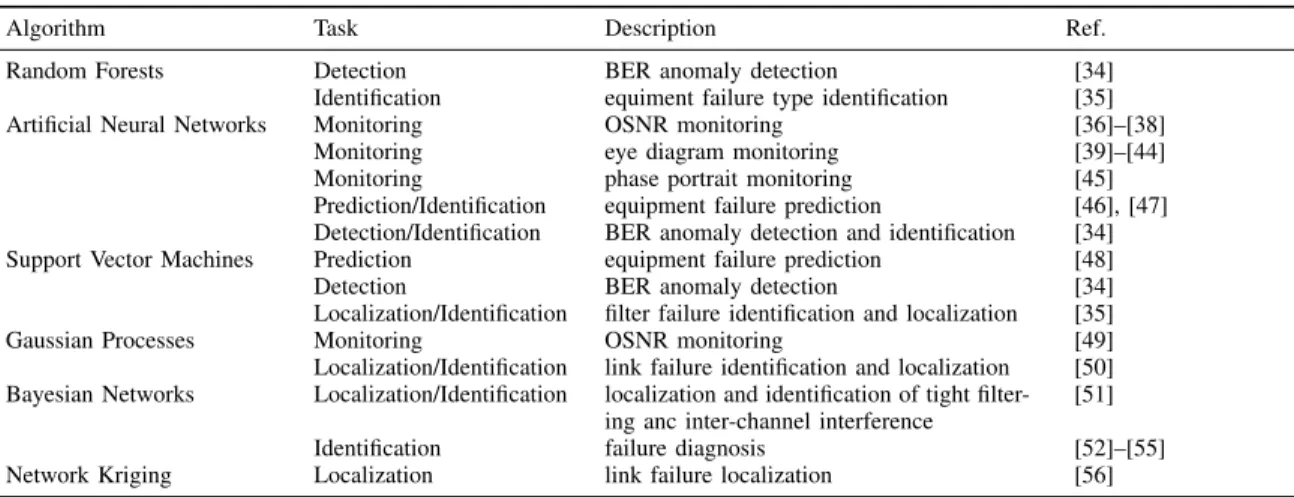
In the following, we describe the various ONFM procedures, and overview some of the existing work addressing ONFM by means of ML algorithms. A summary of this overview is provided in Table I, where we map some existing work with the adopted ML algorithms, as described in Sec. III with the ONFM tasks described in the following subsections.

Note that the interest in automation of ONFM has started several years ago, and even standardizations, in the early 2000s, had been issued to define automatic procedures, e.g., based on events-correlation [33], which can partially replace human intervention in failure management. However, tradi-tional automated approaches are based on static and often simplistic rules, not suitable for modern optical networks, which are characterized by high dynamics and a large amount of diverse network management parameters. In this view, ML is a promising technique to dynamically adapt failure management procedures to the progressively changing network conditions, thanks to its ability of automatically learning from the observed network data.

A. Optical Performance Monitoring (OPM)

During a lightpath’s lifetime, various transmission-performance parameters are constantly controlled by dedicated monitors installed at optical receivers (especially in coherent receivers [57]) or in other strategic points (e.g., in regenerators or intermediate nodes traversed by a lightpath). Typically monitored parameters are, e.g., pre-Forward Error Correction BER (preFEC-BER), OSNR, Polarization Mode Dispersion (PMD), Polarization-dependent loss (PDL), State of Polarization (SOP) in the Stokes space, Chromatic Dispersion (CD) and statistics extracted from the eye diagram. Degradation in one or more of such performance indicators may lead to a failure, unless proper lightpath adjustment is triggered to restore signal quality without service disruption. For example, whenever OPM results in the observation of signal quality degradation, ON operators may adjust some optical parameters at the transmission side (such as, e.g., modulation format, launch power, etc.) or even along the lightpath route (e.g., by activating dispersion compensator modules) to prevent lightpath failure.

Current big-data-analysis techniques enable real-time col-lection, processing and storage of enormous volumes of ONFM data, as demonstrated in the field trial in [36]. On top of this, ML offers powerful tools to perform OPM thanks to the capability of automatically learning complex mapping between samples or features extracted from the received symbols and channel parameters. The most widely used ML tools for OPM

7

Optical Performance

Monitoring and Early-DetectionFailure Prediction DetectionFailure LocalizationFailure Failure MagnitudeEstimation

Failure Prevention Failure Recovery

Failure Identification

Optical Network

Failure Management

Proactive

approaches

approaches

Reactive

Fig. 6: Taxonomy of Optical Network Failure Management. TABLE I: Different use cases in ONFM and their characteristics.

Algorithm Task Description Ref.

Random Forests Detection BER anomaly detection [34]

Identification equiment failure type identification [35]

Artificial Neural Networks Monitoring OSNR monitoring [36]–[38]

Monitoring eye diagram monitoring [39]–[44]

Monitoring phase portrait monitoring [45]

Prediction/Identification equipment failure prediction [46], [47] Detection/Identification BER anomaly detection and identification [34] Support Vector Machines Prediction equipment failure prediction [48]

Detection BER anomaly detection [34]

Localization/Identification filter failure identification and localization [35]

Gaussian Processes Monitoring OSNR monitoring [49]

Localization/Identification link failure identification and localization [50] Bayesian Networks Localization/Identification localization and identification of tight

filter-ing anc inter-channel interference

[51]

Identification failure diagnosis [52]–[55]

Network Kriging Localization link failure localization [56]

are ANNs, which can be fed either with the statistical features of monitored data, or directly with the raw monitored data. Ex-amples of features are Q-factor, closure, variance, root-mean-square jitter and crossing amplitude, extracted from power eye diagrams [39]–[42], [58], [59] and phase portraits [45], asyn-chronous constellation diagrams including transitions between symbols [39], or histograms of the asynchronously sampled signal amplitudes [41], [42]. When directly fed with raw monitored data, ANNs require complex architectures with a high number of neurons and hidden layers and a massive amount of training data to enable automatic extraction of signal quality indicators, such as PMD, PDL, CD, etc. [37], [38], whereas using pre-computed input features allows for the adoption of simpler ANN structures, which can be trained with smaller datasets.

Alternative learning approaches based on Gaussian pro-cesses have also been proposed [49], which show reduced complexity with respect to ANNs, increased robustness against noisy inputs and easier integration within control plane.

B. Failure Prediction and Early-Detection

In some cases, signal quality cannot be simply restored by adjusting transmission parameters as seen in the previous subsection, as signal may keep degrading until a failure occurs. This gradual signal degradation is often referred to as

soft-failure, as opposed to hard-failures, where signal is totally disrupted due to unpredictable events (e.g., a sudden fiber cut). In such cases, prompt detection of soft-failuresbeforea critical threshold is violated is essential as it would allow the operator to gain precious time to devise effective countermeasures. As an example of the application of such proactive approach, the reader is referred to [60], where the authors propose a cloud service restoration strategy which exploits forecasts of link failures in an optical cloud infrastructure.

Several ML algorithms for anomaly detection can be applied directly in the time series of monitored parameters (see Fig. 7) even when their values are still within tolerable ranges. In Fig. 7 we report a simplified graphical representation of the time series of different types of failures. Note that only the “gradual drift” represents a predictable soft-failure, corresponding to a gradual pre-FEC BER degradation due slow filter misalignment. Conversely, both “signal overlap” and “cyclic drift” result in a more sudden degradation of pre-FEC BER, hence predicting such failures is more challenging. Threshold-based approaches for early-failure detection have been proposed to detect fiber deterioration before the occur-rence of a break [62] or to identify anomalous BER trends [61], [63], [64]. In the former scenario, the fiber SOP rotation speed in the Stokes coordinates is monitored and compared to a threshold. If such threshold is exceeded, pre-trigger

Fig. 7: Examples of anomalous pre-FEC BER and received power patterns, depending on different fault types [61].

and post-trigger samples are provided to a ML naive-Bayes classifier, which returns the most likely cause (e.g., fiber bending, shaking, hit or up-and-down events). In the latter scenario, a BER anomaly detection algorithm running at every network node is proposed to identify unexpected BER patterns indicating potential failures along the monitored lightpath. The algorithm takes as input statistics about historical and monitored BER data and returns different types of alerts, de-pending on whether the current BER exceeds given thresholds or remains within pre-defined boundaries. In [48], statistical features of input/output optical power, laser bias current, laser temperature offset and environment temperature are used by an SVM classifier to predict equipment failure. Similarly, optical power levels, amplifier gain, shelf temperature, current draw and internal optical power are used in [46] to forecast failures using statistical regression and ANNs.

C. Failure Detection

Differently from early-detection, which aims at identifying an imminent fault beforethe violation of a certain threshold, the goal of failure detection is to trigger an alert after the values of the monitored parameters exceed the threshold for a sustained period of time.

While, traditionally, these alerts were manually issued, in response to continued growth in network complexity, man-ual management has been progressively replaced by expert systems [33], that were leveraging predefined sets of if-then rules, that could be integrated in the control plane. However, in modern optical networks, failure detection methods based on predefined fixed thresholds and/or if-then rules might still be overly simplified, and not be able to adapt to rapid network dynamics generated, e.g., by on-demand circuit provisioning or by changes in reconfigurable transmission parameters as FEC or modulation format. ML promises to more rapidly evolve and re-adapt failure detection procedures, e.g., by intro-ducing the capability of detectingunknownfailure types (i.e., performing “anomaly detection”) and adapting to changing network condition thanks to periodic algorithm re-training.

In [34] a set of ML algorithms, including Binary SVM, Random Forest (RF), Multiclass SVM, and ANNs have been

!me  

Pre

-­‐FEC  BER

normal  

anomalous  

!me  

Fig. 8: Qualitative pre-FEC BER behaviour vs time under normal and anomalous situations.

used to perform failure detection over an optical-transmission testbed, where pre-FEC BER traces at the receiver are used to detect anomalies in pre-FEC BER behaviour. Two examples of the pre-FEC BER behaviour vs time are shown in Fig. 8 for the cases of normal and anomalous (i.e., corresponding to a failure) BER behaviour. An application of ML algorithms to failure detection will be illustrated in Sec. V.

D. Failure Localization

After a failure has been detected, the failed element (e.g., the node or link responsible for the failure) must be localized in the network. Existing approaches (also based on ML) correlate alarms coming from different receivers and verify if spatial correlation can provide useful information. Data for failure localization can be collected through: i) monitors located at receivers or intermediate nodes of working lightpaths;ii) mon-itors acquired through probe lightpaths that do not carry user traffic and are strategically deployed to help disambiguating the location of a failure.

Correlation methods not relying on probe lightpaths are used in [50], [51]. In particular, in [50], ambiguous localizations are resolved by binary GP classifiers (one for each link suspected of failure), which compute a failure probability after being trained with a dataset of past failure incidents. In [56] NK is adopted to localize failures, assuming that the total number of alarms (i.e., failures) along every lightpath is known. If knowledge on number of failures per lightpath does not allow for unambiguous localization, additional probe lightpaths are installed to increase the rank of the routing matrix. Probe lightpaths are also adopted in [35] for failure localization during the lightpath commissioning testing phase (i.e., prior to the final deployment): low-cost optical testing channels are deployed to collect BER measurements from each traversed node, which are then compared to theoretical BER values. In case of significant discrepancies, a failure alarm is raised for the considered span. The same work also proposes a failure localization algorithm for operative lightpaths, which takes as input some statistical characteristics of the received optical spectrum signal.

E. Failure Identification

Even after failure localization, it might still be complex to understand the exact cause/source of the failure (e.g., inside a network node, the signal degradation can be due to filter misalignment, optical amplifier malfunctioning, etc.). Today,

9

failure identification is still a time-expensive process and consumes lot of precious maintenance human resources [65]. ML classifiers can be used to estimate the most likely failure cause, after being trained with a comprehensive set of time series collected in presence of known failures, as well as during failure-free network operation. For example, probabilistic graphical models such as BNs can be adopted to provide compact representations of distributions (which would be intractably large to be explicitly described) taking advantage of the sparse dependencies among variables.

In [51], statistics about received BER and power are given as input to a BN which outputs a probability of failure occurrence along the ligthpath (thus performing localization, as mentioned in Section IV-D, and additionally returning the most likely cause, either tight filtering or inter-channel interference).

BN have also been proposed for failure diagnosis in GPON/FTTH networks [52], [54], [55]. the ON is represented using a multilayer approach, where the lower layer represents the physical network topology (where nodes are ONTs and ONUs), while the middle layer models local failure propaga-tion inside a single network component (e.g., a single node). Finally the upper layer offers a junction tree representation of the two layers below. Since conditional probabilities in the BN cannot be easily learned in case of missing measurements, in [53] the same authors propose an adaptation of the Expecta-tion MaximizaExpecta-tion (EM) algorithm for Maximum Likelihood Estimation from incomplete data.

Alternatively to BNs, frameworks incorporating multiple ML algorithms have been proposed, where each algorithm focuses on a specific task (e.g., the identification of a particular category of failures), as in [34] and [46], [47] where ANNs are used to perform failure identification in controlled ON testbeds. In [61], the output of the BER anomaly detection mentioned in Section IV-B is fed into a probabilistic algorithm together with historical BER time series, which then returns the most probable failure type from a predefined set of possible causes. Similarly, in [35], features extracted from the spectrum of received signal (including, e.g., power levels across the central frequency and around other cut-off points of the spectrum) are used as inputs of a multi-class decision-tree classifier which outputs a predicted class among three options: normal, laser drift, or filter failure. Then, a more refined diagnosis on laser failures is performed using SVMs to discriminate betwen filter shift or tight filtering, whereas a linear regressor is adopted to estimate laser drift.

A detailed step-by-step description on failure identification, as an extended version of the one in [34], will be provided in Sec. V, where ML classifiers are used to distinguish between two failure causes, i.e., amplifier gain reduction or filter misalignment.

F. Failure Magnitude Estimation

After determining a failure location and cause, the esti-mation of failure magnitude can provide additional informa-tion to understand failure severity. As an example, based on the estimation of failure magnitude, a network operator can decide whether an equipment reconfiguration is sufficient or

equipment reparation, or even substitution, is necessary. Note that, even though we categorize failure magnitude estimation and identification as a reactive approached, they can also be considered as a proactive approached whenever a potential failure is early-detected (i.e., predicted).

ML classification has been already investigated for failure magnitude estimation in [35] where, in addition to fault local-ization and identification algorithms (respectively discussed in Sections IV-D and IV-E), the authors adopt a linear regression model to estimate failure magnitude in the case of filter shift, filter tightening and laser drift failures, using as features var-ious frequency-amplitude points extracted from optical signal spectrum at the receiver.

Preliminary results on failure magnitude estimation will be provided in Sec. V for the optical amplifier malfunctioning and filter misalignment failures mentioned in Sec. IV-E.

V. A CASE-STUDY FORMLINONFM

The objective of this section is to guide the reader through some of the steps needed to develop a ML-based ONFM framework using a case-study example.

Among the tasks described in Sec. IV, we consider 1) Fail-ure Detection, 2) FailFail-ure Identification, and 3) FailFail-ure Mag-nitude Estimation, all performed by analyzing BER traces1

by means of a ML-based multi-stage approach (summarized in Fig. 9). We describe how we designed our ML-based approaches (e.g., adopted algorithms, selection of hyper-parameters, cross-validation methods, etc.), and then show illustrative numerical results obtained on a controlled testbed.

A. Design of ML-based Modules for Failure Management Data preprocessing and windows formation: As first oper-ation, BER data as those in Fig. 8 shall be prepared to be analyzed by ML algorithms. This procedure is called Data preprocessing and generically consists of transforming raw data, e.g., raw information from network monitors, into a more “tractable” format that can be handled by ML algorithms. A good practice when performing data preprocessing is to visualize the collected data, e.g., by plotting the data in a 2D or 3D space, and to perform outlier removal and/or features normalization. Note that, in case the problem is characterized by a N-dimensional features space (N > 3), data preprocessing can also include dimensionality-reduction, e.g., performed through Principal Component Analysis (PCA) [11], which allows to transform the features space and enable data visualization into a 2D or 3D space.

After data preprocessing, we prepare sets of contiguous

BER windows, i.e., groups of consecutive BER samples,

characterized by two main parameters:i)TBER, i.e., the time between two consecutive BER observations in the window, and

ii) window size, i.e., its time-duration, W. The idea is that, analyzing different consecutive BER windows at the receiver, in case one or more failures are observed, a failure alarm can be issued by the network operator, and the failure cause and its magnitude can be estimated. Note that different windows

may overlap, e.g., if window “a” contains samples from #1 to #15, window “b” can contain samples #2 to #16.

As shown in Fig. 9,givena BER-window, the objective of the ML-based framework is to determine:

1) If the window corresponds to a failure (failure de-tection); as shown in box 1 of Fig. 9, this represents a binary classification problem, i.e., either the window corresponds to a failure or not; only in case the window is classified as corresponding to a failure, it will be given as input to the next step 2.

2) What is the failure cause(failure identification); when a failure is detected, the BER window will be classified by the failure identification module (box 2 in Fig. 9); in our illustrative numerical analysis, two different failure causes will be distinguished, i.e., OSNR reduction driven by undesired excessive attenuation along the path, due to, e.g., optical amplifier malfunctioning (Low-gain), and excessive signal filtering, due to, e.g., filter misalign-ment in a multi-span optical fiber transmission system (Filtering); therefore, also in this case the ML-module is a binary classifier.

3) What is the failure magnitude (failure magnitude estimation); according to the failure cause identified in step 2, a proper ML-based classifier is triggered, which analyzes the BER-window and provides the range of the failure magnitude for Low-gain and Filtering failures, respectively. In both cases (see boxes 3a and 3b in Fig. 9), the ML modules represent multi-class classifiers; that is, in case of Low-gain failure, module 3a estimates the failure magnitude as belonging to class “[1-4] dB”, “[5-7] dB”, or “[8-10] dB”; on the other hand, for Filtering failure, module 3b selects one of the following classes estimates the failure magnitude as belonging to class “[26-30] GHz”, “[32-36] GHz”, or “[38-46] GHz”. Note that, given the 3-steps workflow above, a misclassifi-cation in a given step will induce a misclassifimisclassifi-cation also in the subsequent steps, however, such cascaded misclassification errors will be accounted only once when evaluating the overall classification accuracy.

1) BER-Window Features and Labels: To train the various ML algorithms, several BER windows are used, each charac-terized by a feature vectorx and an output labely.

The same set of features (i.e., the same feature vector x) is used for the detection, identification and magnitude estimation tasks. More specifically, for each BER-window, we consider the following 16 features (i.e., x={x1, ..., x16}):

• x1=min: minimum BER value in the window;

• x2=max: maximum BER value in the window;

• x3=mean: mean BER value in the window;

• x4=std: BER standard deviation in the window;

• x5=p2p: “peak-to-peak” BER, i.e.,p2p=max−min;

• x6=RM S: BER root mean square in the window;

• x7÷x16: the ten strongest spectral components in the

window, extracted by applying Fourier transform. On the other hand, each BER-window is characterized by a vector of labels, i.e., y = {y1, y2, y3}, where each of the

three components in the output vectory is used for only one specific task, as shown in Fig. 9. Namely,

• forfailure detection, a univariate binary label is used for each window, i.e.,y1∈ {0; 1}, wherey1= 0corresponds

to a normal BER-window, whereas y1 = 1 corresponds

to ananomalousBER window;

• forfailure identification, again a univariate binary label is used for each window, i.e.,y2∈ {0; 1}, wherey2= 0

corresponds to a Low-gain failure, whereas y2 = 1

corresponds to a Filtering failure; note that, for the failure identification problem, ML training is performed by considering only anomalous BER-windows;

• for failure magnitude estimation, a multi-class output

label is used for each window, i.e., y3 ∈ {r1;r2;r3}, wherey3=ri,i= 1,2,3indicates thei-th range of Low-gain (respectively, Filtering) failure magnitude range, expressed in dB (respectively, GHz); note that we de-veloped and trained twodifferentML-based modules for the Low-gain and Filtering failures, each trained with the corresponding set of BER windows. Moreover, note that we evaluate the overall performance of the framework by considering different ranges of failure magnitude; more specifically, we consider the cases of “2-ranges” and “3-ranges”. In the former case, output label for each window is in the form of y3 ∈ {r1;r2}, while in the

latter case each label can take one out of three possible values, i.e.,y3∈ {r1;r2;r3}, as shown in the outputs of blocks 3a and 3b in Fig. 9. Consequently, as shown in Fig. 9, in the “3-ranges” scenario, the BER window is fed into the 3-steps ONFM framework, where the possible output classes are 7: 1)No-failure, 2)Low-gain-[range1] dB, 3)Low-gain-[range2] dB, 4)Low-gain-[range3] dB, 5)Filtering-[range1] GHz, 6)Filtering-[range2] GHzor 7)Filtering-[range3] GHz. Similarly, for the“2-ranges” case, a total of 5 output classes will be available. In the following we provide more details on the ML algorithms adopted to perform the three tasks and we answer to some practical questions as:i)how often should we collect

BER samples to have an accurate BER detection? ii) how

many consecutive anomalous windows should we wait before issuing a failure alarm? Moreover, for each algorithm, we study the trade-off between classification accuracy and algo-rithm complexity, by varying the value of the window time-duration,W (largeW leads to higher accuracy, but also higher computational time).

2) Failure Detection ML Algorithms: The Failure Detection module has been developed using one-class SVM classifier. Other types of ML classification algorithms (Random Forest (RF), Multiclass SVM, and artificial neural network (ANN)) have also been tested and compared with the one-class SVM, in terms of accuracy and training phase duration. Note that, while the one-class SVM is an unsupervised classifier, all the other approaches are supervised (see Sec. III)2.

2_{In our experiment, for the one-class SVM case, we use only “normal”}

BER data (i.e., BER values not resulting into a failure), whereas for the supervised cases we use a larger data-set, consisting of “normal” BER data and all different types of failures.

11

1. Failure Detection BER-window corresponds to a

failure?

3a. Failure Magnitude Estimation (Low-gain)

What is the attenuation range? 2. Failure Identification

What is the causeof failure for this window?

time BER BER Window W TBER Yes No 3b. Failure Magnitude Estimation (Filtering) What is the filtering

range?

Output 1) No-failure

& continue BER monitoring considering next window

Low-gain Filtering [1-4] dB [5-7] dB [8-10] dB [26-30] GHz [32-36] GHz [38-46] GHz (x,y3) (x,y2) (x,y₁) Output 2) Low-gain [range1] Output 3) Low-gain [range2] Output 4) Low-gain [range3] Output 5) Filtering [range1] Output 6) Filtering [range2] Output 7) Filtering [range3] Fig. 9: 3-steps Optical Network Failure Management (ONFM) block diagram (assuming “3-ranges” scenario for failure magnitude estimation).

The one-class SVM has been implemented with a radial basis function kernel [11], whereas third-degree polynomial kernel has been used for the multiclass SVM classifier; Gini impurity [11] has been used as splitting criteria for decision trees in the RF algorithm; an ANN with single hidden layer, consisting of 10 hidden neurons with Relu activation function, has been used. Hyperparameters in all the algorithms, e.g., number of hidden layers and nodes in the ANN, number of decision trees in RF, kernel in the SVMs, etc., have been selected using cross-validation. Specifically, for each of the aforementioned algorithms, several models have been developed, each with a specific hyperparameters settings. The resulting model is selected as the one providing the best classification accuracy, evaluated using the LOOCV technique. Note that, in this paper, the results provided in the following analyses are obtained adopting one-class SVM for the Failure Detection phase. The performance comparison between the various ML algorithm is out of the scope of this paper.

3) Failure Identification ML Algorithm: Failure Identifica-tion has been implemented using an ANN with two hidden layers, each with 5 hidden neurons, and with Relu activation function. Also in this case cross-validation has been used to fine-tune hyperparameters, i.e., the number of hidden layers and neurons, and the activation function.

4) Failure Magnitude Estimation ML Algorithm: To

esti-mate failure magnitude we adopted ANNs for both low-gain and filtering failures (boxes 3a and 3b in Fig. 9, respectively). For both modules, we used ANNs with a single hidden layer, considering Relu activation function in the hidden nodes. As for the number of hidden neurons, cross-validation has been used to find a proper balance between model accuracy and training duration, and it depends on the number of output labels under consideration. Specifically, we consider ANNs with a number of hidden neurons ranging between 80 and 90 for the“2-ranges”and“3-ranges”scenarios, for both filtering and low-gain magnitude estimation cases.

TX _WSSBV RX

80km

E1 E2

Fig. 10: Testbed setup. B. Results

Testbed setup. To perform our analysis, BER traces have been obtained over an experimental testbed as shown in Fig. 10. Measurements were performed on an 80 km Ericsson OTU-4 transmission system employing PM-QPSK modulation at 100 Gb/s line rate. Signal is transmitted on central frequency of 192.5 THz (i.e., 1557.36 nm) using 50 GHz spectrum width. The end-to-end system is constituted by a series of Erbium Doped Fiber Amplifiers (EDFA) followed by Variable Optical Attenuators (VOAs). Note that the numerical analysis in this section is based on a simplified point-to-point testbed and can only represent a proof of concept for the application of ML to different ONFM use cases. Considering more complex and realistic ON scenarios, e.g., based on a ring/mesh physical topology and a richer set of ligthpaths, would affect the conclusion of such analysis, e.g., due to the emergence of non-linear effects on signal propagation of interfering lightpaths. Further analysis considering more complex topologies and traffics (and others as, e.g., the selection of most effective ML algorithms, or the selection of other input features among the monitored optical parameters, such as the OSNR) are out of the scope of this paper and are left for future work.

A Bandwidth Variable-Wavelength Selective Switch (BV-WSS) is configured to introduce narrow filtering or additional attenuation with the intent to emulate two possible impair-ments that cause BER degradation, i.e., filter misalignment and an undesired amplifier-gain reduction. We have formed our dataset starting from a “normal” (i.e., non-failed) con-dition, where a frequency slot of 50 GHz (i.e., no narrow

0 1 2 3 4 5 60 65 70 75 80 85 90 95 100

Window size [minutes]

Accurac y [%] Detection Identification Mag-Est (Low-gain) Mag-Est (Filtering) ONFM

Fig. 11: Classification accuracy vs window size for different tasks in isolation and for the overall ONFM (“2-ranges” scenario,TBER= 2s).

filtering) and a 0 dB attenuation (i.e., no extra attenuation) are considered. Additional filtering and low-gain failures are gradually imposed through the BV-WSS, by reducing its bandpass spectrum from 46 GHz to 26 GHz at steps of 2 GHz (maintaining a fixed central frequency) and by applying extra attenuation (i.e., to emulate optical amplifier gain reduction) between 1 and 10 dB ad fixed steps of 1 dB. Thus, we gather data representing two different BER-degradation causes as well as different magnitude of gain reduction and filtering, over which we could train and test our ML-based modules.

For each combination of the above mentioned filtering and gain reduction values (i.e., 46-to-26 GHz filtering with 2 GHz-steps, and 1-to-10 dB gain reduction with 1 dB-steps, respectively) and including also normal BER condition (i.e., 50 GHz spectrum and 0 dB gain-reduction), we collected BER samples for one hour with a sampling interval of 2 seconds. Therefore, our overall dataset consists of 24-hours of BER samples collected every 2 seconds, totalling an amount of 43200 BER points. Note that, as we consider BER-windows as training and test data instead of individual BER points, the number of (x,y) points depends on the considered values of BER sampling period,TBER, and window time-duration,W. We first assess the performance of the overall ONFM frame-work considering the case of“2-ranges”for failure magnitude estimations. To this end, we compare the performance of the overall ONFM with that of the “isolated” failure detection, identification and magnitude estimation modules (i.e., modules 1, 2, 3a and 3b in Fig. 9, respectively).

Performance comparison.

Common metrics to evaluate the performance of ML al-gorithms are the classification accuracy and the training-phase duration (that represents the complexity of the ML algorithm). Here, since the amount of data in the different classes is not ncessarly balanced, we also use other metrics as, precision, recall andF-score(see Section III).

Fig. 11 shows the overall accuracy of the whole ONFM framework, and of each of its components, for different values of window durationW, in the “2-ranges” scenario. As expected, accuracy increases with window size in all cases. As expected, failure detection task is the most efficient as it

0 1 2 3 4 5 60 65 70 75 80 85 90 95 100

Window size [minutes]

Accurac y [%] Mag-Est (Low-gain) Mag-Est (Filtering) ONFM

Fig. 12: Classification accuracy vs window size for different tasks in isolation and for the overall ONFM (“3-ranges” scenario,TBER= 2 s).

provides classification accuracy close to 100% with window size above 2.5 minutes. On the other hand, our analysis suggests that, to properly perform failure cause identification, i.e., to distinguish between filter and low-gain failures with reasonably high accuracy, larger window size is needed, i.e., in the order of 5 minutes to reach 90% accuracy. Consider-ing failure-magnitude estimation, we observe that increasConsider-ing window size is more beneficial in the case of filter failures, as demonstrated by the steeper increase of classification accuracy for values ofW above 1.5 minutes. It is worth noting that the overall accuracy of ONFM is highly influenced by the poor performance of the failure identification task, especially when the window size is below 2.5 minutes.

A similar comparison for the “3-ranges” case is shown in Fig. 12. Here curves for the isolated failure detection and failure identification modules are not shown as their accuracy does not depend on the number of classes used in the magnitude estimation tasks, therefore curves are equivalent to the ones observed in Fig. 11. Also in this case we observe high benefit in increasing window size, especially in the filter fail-ure magnitude estimation, where around 100% classification accuracy is reached for window size above 4 minutes.

In Tabs. II and III, for the “2-ranges” scenarios, we show how the Precision (P), Recall (R) and F-score measures vary with increasing window size W, in the cases of low-gain and filtering failure magnitude estimation, respectively. In both cases the F-score steadily increases with window size, despite this is not always the case for P and R, meaning that in any case a good balance between these two metrics is obtained when increasing W. In particular, P shows a decrease in the low-gain failure magnitude estimation case for

W = 250 seconds, whereasR always increases for this task. On the other hand, in the filter failure magnitude estimation

R decreases from 0.97 down to 0.94 for W = 200 seconds, before increasing again up to 0.98 for W = 300 seconds. However, the value ofP in this case always increases, which makes theF-score steadily increase also for this task.

Note that this study considers a single-lightpath system, but other sophisticated optimization can be performed in a more complex network environment, such as, e.g., the selection of

13

TABLE II: Precision (P), Recall (R) andF-score vs window size W (Low-gain failure magnitude estimation).

W [seconds] P R F-score 50 0.84 0.84 0.84 100 0.88 0.88 0.88 150 0.9 0.88 0.89 200 0.92 0.90 0.91 250 0.9 0.93 0.91 300 0.92 0.93 0.92

TABLE III: Precision (P), Recall (R) andF-score vs window size W (Filtering failure magnitude estimation).

W [seconds] P R F-score 50 0.81 0.8 0.8 100 0.85 0.8 0.83 150 0.93 0.97 0.95 200 0.96 0.94 0.95 250 0.98 0.95 0.96 300 0.98 0.98 0.98

monitor placement. If the previous results are confirmed on a network-wide operation scenario, the practical benefits for op-erators would be remarkable. To name few,i) this framework would enable an almost instantaneous troubleshooting (at least for a certain class of common failures) that can significantly reduced time to repair (TTR), and ii) early detection can help eliminate some classes of failure, leading to significant reduction of service downtime.

VI. FUTURERESEARCHDIRECTIONS

A. Open questions

The application of ML in ONFM has only recently gained attention. Several questions remain open regarding the ap-plicability of ML in operational networks, due to scalability problems, network conditions changing too rapidly (or too slowly) to be detected, etc. In this Section, we elaborate on some future research directions in this field.

a) How to deal with changing network conditions: The classical offline supervised learning approach (applied in almost all the studies cited in this paper) should be evolved to cope with time-evolving network scenarios, e.g., in terms of traffic variations or ageing of hardware components. To this aim, semi-supervised and/or unsupervised ML, could be implemented to gradually acquire knowledge from novel input data. Then, the impact of periodic re-training of supervised mechanisms should also be investigated to adapt the ML model to the current network status. Moreover, in this context, ONFM would largely benefit if automatic data labeling is applied after exploiting semi-supervised and/or unsupervised approaches to identify anomalies in dynamic optical networks. As a matter of fact, some papers have already appeared tackling this issue. For example, in [66] the authors concentrate on detecting anomalies in the signal power levels in lightpaths, due to malfunctioning in filters, amplifiers, power equalizer, or even due to jamming attacks. Also in [67] the authors exploit unsupervised learning to detect jamming attacks, by applying optical performance monitoring to correlate the behaviour of

physical layer parameters (such as, e.g., chromatic dispersion, OSNR, BER, etc.) with malicious traffic.

b) How to selectively query the network to obtain useful monitoring information: In several cases, monitored data is expensive to be acquired and shall be extracted/queried only when necessary. Active ML approaches, which can interac-tively ask to observe training data with specific characteristics, could be adopted to reduce the size of datasets required to build an accurate prediction model, thus leading to significant savings in case the data collection process is costly (e.g., when probe lightpaths have to be deployed).

c) How to discover relevant patterns in case of large scale data sets: This point is the logical counterpart of the previous point. For some monitoring systems, the amount of generated data is enormous and the techniques employed to extract useful information shall be extremely scalable (“big data” analysis). Some scalable approaches for big-data analysis are in the area of Association Analysis (AA) (e.g., the a-priori algorithm [68]), and can find hidden relationships in large-scale data. AA could distil the redundant alert information to a single or multiple failure scenarios.

d) Once a failure has been detected, can ML also help making decision on the most appropriate reaction to the fail-ure?: Consider a ML algorithm performing anomaly detection on the monitored BER data at an optical receiver. Assume that the ML algorithm detects an anomalous behavior during a time window covering the last few seconds. What is the best action to be triggered? Should the lightpath be immediately rerouted, or maybe it is sufficient to leverage tunable transceiver to reduce the transmission baud rate/modulation format? These decisions are far from trivial and if ML can help in this context deserves further investigation.

B. Network telemetry: a key enabler for ML in ONs

In this tutorial, we assumed monitored data can be re-trieved from equipment and elaborated in suitable ctrol/management logical elements. In practice, research is on-going to identify the right monitoring and control technologies. For example, in SDN, two main components are required to efficiently support ML applications. First, monitoring param-eters require the definition of common, vendor-neutral YANG models. Specifically, YANG definitions are required for coun-ters, power values, protocol stats, up/down events, inventory, and alarms, originated from data, control, and management planes. Relevant standardization initiatives and working groups on YANG modeling are currently active in IETF, OpenCon-fig [69] and OpenROADM [70]. As of today, YANG models are moderately mature and preliminarily supported by several vendors, but they are not yet completely inter-operable, and this is significantly delaying their deployment in production networks. Second, a streaming telemetry protocol is required to efficiently retrieve data directly from devices to the Teleme-try Collector running ML algorithms [71]. Moreover, telemeTeleme-try should enable efficient data encoding, secure communica-tion, subscription to desired data based on YANG models, and event-driven streaming activation/deactivation. Traditional monitoring solutions (e.g., SNMP) are not adequate, since they