The Burr XII modified Weibull distribution: model, properties and applications

EJASA, Electron. J. App. Stat. Anal. http://siba-ese.unisalento.it/index.php/ejasa/index e-ISSN: 2070-5948

DOI: 10.1285/i20705948v10n1p118

The Burr XII modified Weibull distribution: model, properties and applications

By Mdlongwa et al.

Published: 26 April 2017

This work is copyrighted by Universit`a del Salento, and is licensed un-der aCreative Commons Attribuzione - Non commerciale - Non opere derivate

3.0 Italia License.

For more information see:

DOI: 10.1285/i20705948v10n1p118

The Burr XII modified Weibull

distribution: model, properties and

applications

Precious Mdlongwa

, Broderick O. Oluyede

, Alphonse Amey

,

and Shujiao Huang

a_{Botswana International University of Science and Technology, Department of Mathematics}

and Statistical Sciences, Palapye, BW

b_{Georgia Southern University, Department of Mathematical Sciences, Statesboro, GA, 30460} d_{University of Houston, Department of Mathematics, Houston, TX, 77204}

Published: 26 April 2017

A new distribution called Burr XII modified Weibull (BXIIMW or BMW) distribution is presented and its properties explored. This new distribution contains several new and well known sub-models, including Burr-Weibull, Burr-exponential, Burr-Rayleigh, Burr XII, Lomax modified Weibull, Lomax-Weibull, Lomax-exponential, Lomax-Rayleigh, Lomax, Lomax-Weibull, Rayleigh, and exponential distributions. Some structural properties of the proposed distribution including the shapes of the hazard rate function, moments, con-ditional moments, moment generating function, skewness and kurtosis are presented. Mean deviations, Lorenz and Bonferroni curves, R´enyi entropy and the distribution of the order statistics are given. Maximum likelihood estimation technique is used to estimate the model parameters and finally applications of the model to real datasets are presented to illustrate the use-fulness of the proposed distribution.

Keywords: Weibull distribution, Structural properties, Failure-time, Max-imum likelihood estimation.

∗

Corresponding author: [email protected].

c

Universit`a del Salento ISSN: 2070-5948

1 Introduction

Burr XII and Weibull distributions are two of the most important and most widely used distributions for lifetime as well as the wealth data analysis and modeling. Burr Type XII is a member of a system of continuous distributions introduced by Burr (1942). The flexibilities of Burr XII distribution were studied by Hatke (1949), Burr and Cislak (1968), Rodrigues (1977) and Tadikamalla (1980). Burr XII distribution has been used in many applications such as actuarial science, quantal bio-assay, economics, forestry, toxicology, life testing and reliability. According to Soliman (2005), this distribution covers shapes that is characteristic of a large number of distributions. The versatility and flexibility of the Burr XII distribution makes it quite attractive as a tentative model for data whose underlying distribution is unknown.

Weibull distribution by Weibull (1951) on the other hand is one of the most important and widely used lifetime distributions in reliability engineering and lifetime analysis. This is because of its flexible ability to fit a variety of data. However, it does not exhibit bathtub shape for its hazard rate function and as a result many researchers have proposed modifications and generalizations of the Weibull distribution to accommodate bathtub shaped hazard rates and non-monotone hazard rates in general. Among the various extension and modified forms of the Weibull distribution are the exponentiated Weibull family presented by Mudholkar and Srivastava (1993), generalized Weibull by Pham and Lai (2007), Gurvich et al. (1997), modified Weibull distribution by Lai et al. (2003) and the gamma generalized modified Weibull distribution given by Oluyede et al. (2015). The modified Weibull distribution of Lai et al. (2003) is one of the most important modification of the Weibull distribution. This distribution has increasing or bathtub-shaped failure rate functions.

The primary motivation for developing this distribution is the versatility and flexibility obtained from the product of the reliability or survival functions of the Burr XII and modified Weibull distribution via the use of competing risks to obtain a new model called the Burr XII modified Weibull distribution with desirable properties including hazard function that exhibits increasing, decreasing, bathtub and upside down bathtub shapes. The results in this paper are organized in the following manner. The new model called Burr XII modified Weibull (BXIIMW or BMW) distribution, its sub-models, quantile function, hazard and reverse hazard functions are given in section 2. In section 3, moments, moment generating function and conditional moments are presented. Mean deviations, Lorenz and Bonferroni curves are given in section 4. Section 5 contain results on R´enyi entropy, density of the order statistics and L-moments. Maximum likelihood estimates of the model parameters are given in section 6. A Monte Carlo simulation study to examine the bias and mean square error of the maximum likelihood estimates is presented in section 7. Section 8 contains applications of the new model to real data sets. A short concluding remark is given in section 9.

2 Burr XII Modified Weibull Distribution

In this section, the model, hazard and reverse hazard functions and quantile function are presented. First, the modified Weibull and Burr XII distributions are presented. The cumulative distribution function (cdf) of the modified Weibull (MW) distribution of Lai et al. (2003) is given by

F_{M W}(y;α, β, λ) = 1−exp(−αyβeλy), y≥0, α >0, β >0, λ≥0. (1)

Note thatαcontrols the scale of the distribution,β controls the shape, whereasλcan be considered to be an accelerating factor in the imperfection time and a factor of fragility in the survival of the individual as time increases. The cdf of Burr XII distribution is given by

GB(y;c, k) = 1−(1 +y

c₎−k_{, y≥0, k >0, c >0, (2)} wherek and care shape parameters.

The reliability function of the new distribution called Burr XII Modified Weibull (BMW) distribution (obtained via the use of competing risk model) is constructed by combining the reliability functions for both the Burr XII and modified Weibull distribu-tions. The resulting reliability or survival function is given by

F_{BM W}(y;c, k, α, β, λ) = (1 +yc)−ke−αyβeλy, c, k, α, β >0 and λ≥0. (3)

The cdf of the new BMW distribution is given by FBM W(y;c, k, α, β, λ) = 1−(1 +y

c₎−k_e−αyβ_eλy

, (4)

for c, k, α, β > 0 and λ ≥ 0. The corresponding probability density function (pdf) is given by

fBM W(y;c, k, α, β, λ) = (1 +y

c₎−k−1_e−αyβ_eλyn

kcyc−1+ (1 +yc)αeλyyβ−1(β+λy)

o

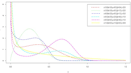
(5) forc, k, α, β >0 andλ≥0.Plots of the pdf for selected values of the model parameters are given in Figure 1. The plots suggests that the pdf can be right skewed or decreasing among many other shapes for the selected values of the model parameters.

2.1 Quantile Function

In this sub-section, the quantile function of the BMW distribution is presented. The quantile function can be obtained by inverting FBM W(y) = 1−u, 0≤u≤1,where

F_{BM W}(y) = (1 +yc)−ke−αyβeλy. (6)

The quantile function is obtained by solving the non-linear equation

Figure 1: Plots of BMW PDF

using numerical methods. Consequently, random number can be generated based on equation (7). Table 1 lists the quantile for selected values of the parameters of the BMW distribution.

Table 1: BMW Quantile for Selected Values

(c, k, α, β, λ) u (3.0,3.0,0.5,0.4,2.0) (3.0,3.0,0.5,1.5,2.0) (0.9,2.0,0.5,1.5,5.0) (0.5,2.0,2.0,4.0,1.0) (0.5,0.5,2.0,4.0,1.0) (1.0,0.3,0.1,0.3,0.9) 0.1 0.01853977 0.2141278 0.03726958 0.002951125 0.05499965 0.1469918 0.2 0.08512607 0.2964359 0.08408788 0.01393109 0.2699589 0.4338763 0.3 0.1678449 0.3591675 0.1359876 0.03811902 0.4295427 0.7711961 0.4 0.245917 0.4141029 0.1896706 0.08463554 0.5171622 1.124044 0.5 0.3183341 0.4660199 0.2424022 0.1704162 0.5817035 1.470701 0.6 0.3885882 0.5181238 0.2931962 0.3138966 0.6370646 1.806173 0.7 0.4613197 0.5738216 0.3428492 0.4715588 0.6896507 2.138562 0.8 0.5436832 0.6385877 0.3944155 0.5976683 0.7450474 2.488656 0.9 0.654306 0.7270882 0.4556709 0.716097 0.813945 2.911513

2.2 Hazard and Reverse Hazard Functions

In this sub-section, the hazard and reverse hazard functions of the BMW distribution are presented. Graphs of the hazard function for selected values of the model parameters

are also presented. The hazard and reverse hazard functions are given by h_F(y) = fBM W(y)

F_{BM W}(y)

= (1 +y

c₎−k−1_e−αyβ_eλy

kcyc−1+ (1 +yc)αeλyyβ−1(β+λy) (1 +yc₎−k_e−αyβ_eλy

= kcyc−1(1 +yc)−1+αeλyyβ−1(β+λy), (8) and

τ_F(y) = fBM W(y) F_{BM W}(y)

= (1 +y

c₎−k−1_e−αyβ_eλy

kcyc−1+ (1 +yc)αeλyyβ−1(β+λy)

1−(1 +yc₎−k_e−αyβ_eλy , (9) respectively.

The limiting behavior of the hazard function of the BMW distribution, which can be readily established is as follows:

• Note that, lim y→0hF(y) =                ∞ 0< c <1, β = 1, α c >1, β = 1, α+k c= 1, β = 1, k c= 1, β >1, 0 c >1, β >1.

• Forβ >0 and c >0,limy→∞hF(y) =∞.

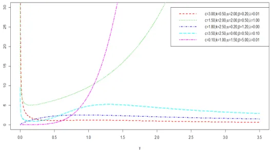
Plots of the hazard function are given in Figure 2. The graphs exhibit decreasing, increasing, bathtub followed by upside down bathtub, and bathtub shapes for the selected values of the model parameters. This very attractive flexibility makes the BMW hazard function useful and suitable for non-monotonic empirical hazard behaviors which are more likely to be encountered in practice or real life situations.

2.3 Some Sub-models

There are several new as well as well known distributions that can be obtained from the BMW distribution. The sub-models include the following distributions:

• When α→0+,we obtain Burr XII or Burr (B) distribution.

• When λ= 0,we obtain Burr-Weibull (BW) distribution.

• Ifλ= 0 and β = 1,we obtain the Burr-Exponential (BE) distribution.

Figure 2: Plots of BMW Hazard Function

• Ifc= 1,we obtain the Lomax-modified Weibull (LMW) distribution.

• Ifc= 1, λ= 0 and β = 2,we obtain the Lomax-Rayleigh (LR) distribution.

• Ifc= 1, λ= 0 and β = 1,we obtain the Lomax-Exponential (LE) distribution.

• Ifk→0+ _{and λ= 0,we obtain Weibull (W) distribution.}

• Ifk→0+, λ= 0 andβ = 2,we obtain Rayleigh (R) distribution.

• Ifk→0+, λ= 0 andβ = 1,then we have the Exponential (E) distribution.

• Ifk→0+,we obtain the modified Weibull (MW) distribution.

• Ifβ = 1,then we obtain the Burr-modified Exponential (BME) distribution with cdf given by

F(y) = 1−(1 +yc)−ke−αyeλy, (10) forc, α, k >0, λ≥0 andy ≥0.

• If β = k = 1 and λ = 0, then the BMW cdf reduces to the two parameter Log-logistic Exponential (LLoGE) distribution given by

F(y) = 1−(1 +yc)−1e−αy, (11) forc, α >0,andy≥0.

• If λ = 0, k = 1 and β = 2, then the BMW cdf reduces to the two parameter Log-logistic Rayleigh (LLoGR) model with the cdf

F(y) = 1−(1 +yc)−1e−αy2, (12)

forc, α >0 and y≥0.

• If λ = 0, and k = c = β = 1, then the BMW cdf reduces to the one parameter model with the cdf

F(y) = 1−(1 +y)−1e−αy, (13) forα >0 and y≥0.

3 Moments, Moment Generating Function and

Conditional Moments

Moments are very important and necessary in any statistical analysis, especially in appli-cations. Moments can be used to study the most important features and characteristics of a distribution (e.g. central tendency, dispersion, skewness and kurtosis). In this sec-tion, moments, moment generating function (mgf) and conditional moments are given for the BMW distribution. Measures of dispersion, skewness and kurtosis, as well as tables of the first six moments for selected values of the model parameters are also presented.

3.1 Moments

The rth moment of the BMW distribution is given by

E(Yr) = Z ∞ 0 yrf_{BM W}(y)dy = Z ∞ 0 yr(1 +yc)−k−1e−αyβeλy n

kcyc−1+ (1 +yc)αeλyyβ−1(β+λy)

o dy = ∞ X m,p=0 (−1)mαm(mλ)pkc m!p! Z ∞ 0 yr+c+mβ+p−1(1 +yc)−k−1dy + ∞ X m,p=0 (−1)mαm+1((m+ 1)λ)pβ m!p! Z ∞ 0 yr+mβ+β+p−1(1 +yc)−kdy + ∞ X m,p=0 (−1)mαm+1(m+ 1)pλp+1 m!p! Z ∞ 0 yr+mβ+β+p(1 +yc)−kdy.

Letx= (1 +yc)−1,then E(Yr) = ∞ X m,p=0 (−1)mαm(mλ)pk m!p! Z 1 0 xk+3−1c(r+mβ+p)(1−x) 1 c(r+mβ+p)dx + ∞ X m,p=0 (−1)m_αm+1_{β((m+ 1)λ)}p m!p!c Z 1 0 xk+3−1c(r+mβ+p)(1−x) 1 c(r+mβ+β+p)−1dx + ∞ X m,p=0 (−1)mαm+1(m+ 1)pλ)p+1 m!p!c Z 1 0 xk+3−1c(r+mβ+β+p+1)(1−x) 1 c(r+mβ+β+p+1)−1dx = ∞ X m,p=0 (−1)mαm(mλ)pk m!p! B k−1 c(r+mβ+p−4c), 1 c(r+mβ+p+c) + ∞ X m,p=0 (−1)mαm+1β((m+ 1)λ)p m!p!c B k−1 c(r+mβ+p−4c), 1 c(r+mβ+β+p) + ∞ X m,p=0 (−1)mαm+1(m+ 1)pλp+1 m!p!c × B k−1 c(r+mβ+β+p−4c+ 1), 1 c(r+mβ+β+p+ 1) , (14) whereB(a, b) =R1 0 t

a−1_(1−t)b−1_{dtis the beta function. The moment generating function}

of the BMW distribution is given by E(etY) = P∞

i=0t

i i!E(Y

i_{), where E(Y}i_{) is given} above.

The coefficients of variation (CV), Skewness (CS) and Kurtosis (CK) can be readily obtained. The variance (σ2), coefficient of variation (CV), coefficient of skewness (CS) and coefficient of kurtosis (CK) are given by

σ2 =µ0₂−µ2, CV = σ µ = p µ0₂−µ2 µ = s µ0₂ µ2 −1, (15) CS= E (X−µ)3 [E(X−µ)2_]3/2 = µ0₃−3µµ0₂+ 2µ3 (µ0₂−µ2₎3/2 , (16) and CK = E (X−µ)4 [E(X−µ)2_]2 = µ0₄−4µµ0₃+ 6µ2µ0₂−3µ4 (µ0₂−µ2₎2 , (17)

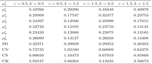
respectively. Table 2 lists the first six moments of the BMW distribution for selected values of the parameters, by fixing α = β = 1.5 and λ = 0.5. Table 3 lists the first six moments of the BMW distribution for selected values of the parameters, by fixing c= 2.0 andk= 1.0.These values can be determined numerically using R and MATLAB.

Table 2: Moments of the BMW distribution for some parameter values;α=β = 1.5 and λ= 0.5. µ0_s c= 0.5, k = 0.5 c= 0.5, k = 1.5 c= 1.5, k = 0.5 c= 1.5, k = 1.5 µ0₁ 0.43766 0.29290 0.48848 0.40979 µ0₂ 0.29569 0.17537 0.32477 0.23753 µ0₃ 0.24297 0.13506 0.25999 0.17015 µ0₄ 0.22732 0.12105 0.23710 0.14145 µ0₅ 0.23433 0.12088 0.23875 0.13165 µ0₆ 0.26090 0.13127 0.26028 0.13408 SD 0.32271 0.29929 0.29352 0.26382 CV 0.73735 1.02180 0.60089 0.64378 CS 0.66650 1.16473 0.67919 0.85869 CK 2.92547 3.86304 3.13235 3.56673

Table 3: Moments of the BMW distribution for some parameter values; c = 2.0 and k= 1.0. µ0_s α= 3.5, β= 1.5, λ= 0.5 α= 3.5, β= 0.8, λ= 0.0 α= 1.0, β= 1.5, λ= 0.2 α= 0.8, β= 3.5, λ= 0.5 µ0₁ 0.31249 0.21032 0.50889 0.68308 µ0₂ 0.13308 0.10248 0.36010 0.54319 µ0₃ 0.06870 0.07905 0.31582 0.47550 µ0₄ 0.04074 0.08507 0.32470 0.44606 µ0₅ 0.02689 0.12021 0.37847 0.44154 µ0₆ 0.01938 0.21511 0.48899 0.45660 SD 0.18823 0.24133 0.31801 0.27675 CV 0.60233 1.14746 0.62491 0.40514 CS 0.74599 2.34797 0.92163 -0.00847 CK 3.36566 11.76067 3.92708 2.45747 3.2 Conditional Moments

For lifetime models, it may be useful to know the conditional moments. Therth condi-tional moment is defined as E(Yr | Y > t). The rth conditional moment of the BMW

distribution is given by E(Yr|Y > t) = 1 F_{BM W}(t) Z ∞ t yrfBM W(y)dy = 1 FBM W(t) Z ∞ t yr[1 +yc]−k−1 ∞ X m=0 (−1)mαmymβemλy m!

× hkcyc−1+ (1 +yc)αyβ−1eλy(β+λy)

i

dy.

(18) Letx = (1 +yc)−1,then the rth conditional moment of the BMW distribution is given by E(Yr|Y > t) = 1 F_{BM W}(t) ∞ X m,p=0 (−1)mαm(mλ)pk m!p! × B_(1+tc₎−1 k−1 c(r+mβ+p−4c), 1 c(r+mβ+p+c) + ∞ X m,p=0 (−1)mαm+1β((m+ 1)λ)p m!p!c × B_(1+tc₎−1 k−1 c(r+mβ+β+p−4c), (r+mβ+β+p) + ∞ X m,p=0 (−1)mαm+1(m+ 1)pλp+1 m!p!c × B_(1+tc₎−1 k−1 c(r+mβ+β+p−4c+ 1), 1 c(r+mβ+β+p+ 1) , whereBy(a, b) = Ry 0 x

a−1_(1−x)b−1_{dxis the incomplete beta function, andc > r+mβ+}

β+p+ 1.The mean residual lifetime function is given by E(Y|Y > t)−t=V_F(t)−t, whereVF(t) is called the vitality function of the distribution function F.

4 Mean Deviations, Lorenz and Bonferroni Curves

Mean deviation about the mean and mean deviation about the median as well as Lorenz and Bonferroni curves for the BMW distribution are presented in this section. Bonferroni and Lorenz curves are widely used tool for analyzing and visualizing income inequality. Lorenz curve,L(p) can be regarded as the proportion of total income volume accumulated by those units with income lower than or equal to the volume y, and Bonferroni curve, B(p) is the scaled conditional mean curve, that is, ratio of group mean income of the population.

4.1 Mean Deviations

The amount of scatter in a population is measured to some extent by the totality of deviations from the mean and median. These are known as the mean deviation about the mean and the mean deviation about the median and are defined by

δ1(y) =

Z ∞

0

|y−µ|fBM W(y)dy and δ2(y) =

Z ∞

0

|y−M|fBM W(y)dy, (19)

respectively, where µ=E(Y) and M =Median(Y) denotes the median. The measures δ1(y) and δ2(y) can be calculated using the relationships

δ1(y) = 2µFBM W(µ)−2µ+ 2 Z ∞ µ yf_{BM W}(y)dy, (20) and δ2(y) =−µ+ 2 Z ∞ M yfBM W(y)dy, (21)

respectively. Whenr= 1,we get the meanµ=E(Y).Note thatT(µ) =R_µ∞yfBM W(y)dy and T(M) =R_M∞yfBM W(y)dy,where

T(µ) = Z ∞ µ yf_{BM W}(y)dy = ∞ X m,p=0 (−1)mαm(mλ)pk m!p! × B_(1+µc₎−1 k−1 c (1 +mβ+p−4c), 1 c(1 +mβ+p+c) + ∞ X m,p=0 (−1)mαm+1β((m+ 1)λ)p m!p!c × B_(1+µc₎−1 k−1 c (1 +mβ+β+p−4c), (1 +mβ+β+p) + ∞ X m,p=0 (−1)mαm+1(m+ 1)pλp+1 m!p!c × B_(1+µc₎−1 k−1 c (mβ+β+p−4c+ 2), 1 c(mβ+β+p+ 2) . Consequently, the mean deviation about the mean and the mean deviation about the

median reduces to

δ1(y) = 2µFBM W(µ)−2µ+ 2T(µ) and δ2(y) =−µ+ 2T(M), respectively.

4.2 Bonferroni and Lorenz Curves

In this sub-section, we present Bonferroni and Lorenz Curves. Bonferroni and Lorenz curves have applications not only in economics for the study income and poverty, but also in other fields such as reliability, demography, insurance and medicine. Bonferroni and Lorenz curves for the BMW distribution are given by

B(p) = 1 pµ Z q 0 yfBM W(y)dy= 1 pµ[µ−T(q)], and L(p) = 1 µ Z q 0 yf_{BM W}(y)dy= 1 µ[µ−T(q)], respectively, where T(q) = Z ∞ q yf_{BM W}(y)dy = ∞ X m,p=0 (−1)mαm(mλ)pk m!p! × B_(1+qc₎−1 k−1 c(1 +mβ+p−4c), 1 c(1 +mβ+p+c) + ∞ X m,p=0 (−1)mαm+1β((m+ 1)λ)p m!p!c × B_(1+qc₎−1 k−1 c(1 +mβ+β+p−4c), (1 +mβ+β+p) + ∞ X m,p=0 (−1)mαm+1(m+ 1)pλp+1 m!p!c × B_(1+qc₎−1 k−1 c(mβ+β+p−4c+ 2), 1 c(mβ+β+p+ 2) , and q=F−1_{(p),0≤p≤1.}

5 Order Statistics, L-Moments and R´

enyi Entropy

The concept of entropy plays a vital role in information theory. The entropy of a random variable is defined in terms of its probability distribution and can be shown to be a good measure of randomness or uncertainty. In this section, we present the distribution of the order statistic, L-moments and R´enyi entropy for the BMW distribution.

5.1 Order Statistics

Order statistics play an important role in probability and statistics. In this sub-section, we present the distribution of the ith order statistic from the BMW distribution. The

pdf of the ith order statistic from the BMW pdff(y) is given by gi:n(y) = n!fBM W(y) (i−1)!(n−i)![FBM W(y)] i−1_[1−F BM W(y)] n−i = n!fBM W(x) (i−1)!(n−i)! n−i X j=0 (−1)j n−i j [F_{BM W}(y)]j+i−1,

and is obtained by using the binomial expansion

[1−F_{BM W}(y)]n−i = n−i X m=0 n−i m (−1)m[F_{BM W}(y)]m, so that gi:n(y) = 1 B(i, n−i+ 1) n−i X m=0 n−i m (−1)m m+i(m+i)[FBM W(y)] m+i−1_f(y) = n−i X m=0 wi,mfm+i(y),

wheref_m+i(y) is the pdf of the exponentiated BMW distribution with parametersc, k, α, β, λ, and m+i.

The tth moment of the ith order statistic from the BMW distribution can be derived via a result of Barakat and Abdelkader (2004) as follows:

E(Y_it_:n) =t n X p=n−i+1 (−1)p−n+i−1 p−1 n−i n p Z ∞ 0 xt−1[1−F_{BM W}(y)]pdy. (22)

Note that by settingx= (1 +yc)−1,we have

Z ∞ 0 xt−1[1−F_{BM W}(y)]pdy = ∞ X m,s=0 (−1)m(αp)m(mλ)s m!s! Z ∞ 0 yt+mβ+s−1(1 +yc)−pkdy = ∞ X m,s=0 (−1)m(αp)m(mλ)s m!s! 1 c × Z 1 0 xpk−1c(t+mβ+s)−1(1−x) t+mβ+s c −1dx = ∞ X m,s=0 (−1)m_(αp)m_(mλ)s m!s! 1 c × B pk−1 c(t+mβ+s), t+mβ+s c . (23)

Consequently, the tth moment of the ith order statistic from the BMW distribution is given by E(Y_it_:n) = t n X p=n−i+1 ∞ X m,s=0 (−1)p−n+i−1 p−1 n−i n p (−1)m(αp)m(mλ)s m!s! 1 c × B pk−1 c(t+mβ+s), t+mβ+s c , (24)

whereB(a, b) =R₀1ta−1(1−t)b−1dtis the complete beta function.

5.2 L-Moments

TheL−moments (Hoskings, 1990) are expectations of some linear combinations of order statistics and they exist whenever the mean of the distribution exits, even when some higher moments may not exist. They are relatively robust to the effects of outliers and are given by λk+1= 1 k+ 1 k X j=0 (−1)j k j E(Yk+1−j:k+1), k= 0,1,2, ... (25)

The L−moments of the BMW distribution can be readily obtained from equation (24). The first four L−moments are given by λ1 = E(Y1:1), λ2 = 1₂E(Y2:2 −Y1:2), λ3 =

1

3E(Y3:3−2Y2:3+Y1:3) and λ4 = 1

4E(Y4:4−3Y3:4+ 3Y2:4−Y1:4),respectively.

5.3 R´enyi Entropy

In this sub-section, R´enyi entropy (R´enyi, 1960) of the BMW distribution is derived. An entropy is a measure of uncertainty or variation of a random variable. R´enyi entropy is an extension of Shannon entropy. R´enyi entropy is defined to be

IR(v) = 1 1−vlog Z ∞ 0 [fBM W(y;c, k, α, β, λ)]vdy , v 6= 1, v >0.

R´enyi entropy tends to Shannon entropy as v → 1. Note that [f(y;c, k, α, β, λ)]v = fv

BM W(y) can be written as f_{BM W}v (y) =

h

kcyc−1+ (1 +yc)αyβ−1eλy(β+λy)

iv × (1 +yc)−kv−ve−vαyβeλy = ∞ X m,r=0 v X p=0 v p (−1)m(vα)mαp[λ(m+p)]r r!m! (kc) v−p × y(r+mβ+pβ+cv−cp−v)(1 +yc)−kv−v+p(β+λy)p = ∞ X m,r=0 v X p=0 p X w=0 v p p w (−1)m(vα)mαp[λ(m+p)]rλwβp−w r!m! (kc) v−p × y(r+mβ+pβ+cv−cp−v+w)(1 +yc)−kv−v+p. Now, Z ∞ 0 f_{BM W}v (y)dy = ∞ X m,r=0 v X p=0 p X w=0 v p p w (−1)m_(vα)m_αp_[λ(m+p)]r_λw_βp−w r!m! (kc) v−p × Z ∞ 0 y(r+mβ+pβ+cv−cp−v+w)(1 +yc)−kv−v+pdy = ∞ X m,r=0 v X p=0 p X w=0 v p p w (−1)m_(vα)m_αp_[λ(m+p)]r_λw_βp−w r!m!c × (kc)v−pB 1 ca ∗ , kv+v−p−1 ca ∗ + 4 ,

where we have used the substitutionsx= (1 +yc)−1anda∗ = (r+mβ+pβ+cv−cp−v+w+ 1). Consequently, R´enyi entropy is given by

IR(v) = 1 1−v log ∞ X m,r=0 v X p=0 p X w=0 v p p w (−1)m(vα)mαp[λ(m+p)]rλwβp−w r!m!c × (kc)v−pB 1 ca ∗ , kv+v−p−1 ca ∗ + 4 , forv6= 1 and v >0.

6 Maximum Likelihood Estimation

Let Y ∼ BM W(c, k, α, β, λ) and ∆ = (c, k, α, β, λ)T be the parameter vector. The log-likelihood `=`(∆) for a single observation of y of Y is given by

`(∆) = −αyβeλy−(k+ 1) log(1 +yc) + log

kcyc−1+ (1 +yc)αyβ−1eλy(β+λy)

The first derivative of the log-likelihood function with respect to the components of the parameter vector∆= (c, k, α, β, λ)T _{are given by}

∂`

∂c = −

c(k+ 1)yc−1 1 +yc +

kyc−1(1 +clog(y)) +αyβ−1eλy(β+λx)yclog(y) kcyc−1_{+ (1 +y}c_)αyβ−1_eλy_(β+λy) ,

∂`

∂k = −log (1 +y

c_{) +} cyc−1

kcyc−1_{+ (1 +y}c_)αyβ−1_eλy_(β+λy), ∂`

∂α =−y

β_eλy₊ (1 +yc)yβ−1eλy(β+λy) kcyc−1_{+ (1 +y}c_)αyβ−1_eλy_(β+λy), ∂`

∂β =−αe

λy_yβ_{log(y) +}αeλy(1 +yc) (yβ−1+ (β+λy)yβ−1log(y)) kcyc−1_{+ (1 +y}c_)αyβ−1_eλy_(β+λy) , and

∂`

∂λ =−αy

β+1_eλy₊ (1 +yc)αyβ−1(yeλy(β+λy+ 1)) kcyc−1_{+ (1 +y}c_)αyβ−1_eλy_(β+λy), respectively.

The total log-likelihood function based on a random sample ofnobservations: x1, x2, ...., xn

drawn from the BMW distribution is given by `∗_n = Pn

i=1`i(∆), where `i(∆), i =

1,2, ..., n is given by equation (26). The equations obtained by setting the above partial derivatives to zero are not in closed form and the values of the parameters c, k, α, β, λ must be found by using iterative methods. The maximum likelihood esti-mates of the parameters, denoted by ˆ∆ is obtained by solving the nonlinear equation (∂`∗n ∂c, ∂`∗n ∂k, ∂`∗n ∂α, ∂`∗n ∂β, ∂`∗n

∂λ)T = 0, using a numerical method such as Newton-Raphson pro-cedure. The Fisher information matrix is given by I(∆) = [Iθi,θj]5X5 = E(− ∂

2_`

∂θi∂θj), i, j = 1,2,3,4,5, can be numerically obtained by MATLAB or R software. The total Fisher information matrix nI(∆) can be approximated by

J( ˆ∆)≈ − ∂ 2_`∗ n ∂θi∂θj ∆= ˆ∆ 5X5 , i, j= 1,2,3,4,5. (27)

For a given set of observations, the matrix given in equation (27) is obtained after the convergence of the Newton-Raphson procedure in MATLAB or R software.

7 Simulation Study

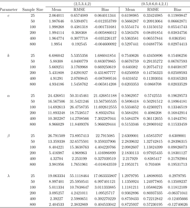
In this section, we examine the performance of the BMW distribution by conducting various simulations for different sizes (n=25, 50, 100, 200, 400, 800) via the R package. We simulate 1000 samples for the true parameters values I : c = 2, k = 5, α = 3, β = 4, λ= 2 andII:c= 0.5, k= 0.6, α= 0.4, β= 2, λ= 1. Table 4 lists the means MLEs of

the five model parameters along with the respective root mean squared errors (RMSE). The bias and RMSEs are given by:

Bias(ˆθ) = Pn i=1θˆi n −θ, and RM SE(ˆθ) = s Pn i=1(ˆθi−θ)2 n ,

respectively. From the results, we can readily verify that as the sample sizenincreases, the mean estimates of the parameters tend to be closer to the true parameter values, since RMSEs decay toward zero.

Table 4: Monte Carlo Simulation Results

(2,5,3,4,2) (0.5,0.6,0.4,2,1)

Parameter Sample Size Mean RMSE Bias Mean RMSE Bias

c 25 2.064011 0.6574089 0.064011344 0.6198985 0.33424985 0.11989847 50 1.987646 0.5394971 -0.012353789 0.5666287 0.20913064 0.06662871 100 1.998268 0.4381318 -0.001731681 0.5554174 0.13150152 0.05541743 200 1.994114 0.368368 -0.005886012 0.5383476 0.08491854 0.03834756 400 1.964774 0.3077718 -0.035226137 0.5363581 0.06557844 0.0363581 800 1.9954 0.192545 -0.004600092 0.5297441 0.04887756 0.02974413 k 25 6.686042 5.5355356 1.686041854 0.7540626 0.43450896 0.15406256 50 5.88308 4.0400779 0.883079865 0.6676759 0.29135272 0.06767593 100 5.669251 3.1769968 0.669250619 0.640382 0.20754712 0.04038197 200 5.431808 2.6291927 0.431807777 0.6250959 0.14756323 0.02509593 400 4.91291 2.0769845 -0.087089516 0.631652 0.11393034 0.03165203 800 4.934186 1.5458762 -0.065814208 0.6203353 0.0868708 0.02033529 α 25 24.426851 50.3145461 21.426851188 0.5962957 0.5742553 0.19629573 50 16.567506 31.5421246 13.567505535 0.5896418 0.50291512 0.18964181 100 14.692613 26.4758735 11.692612555 0.5334652 0.42369271 0.13346519 200 11.893248 18.7538517 8.89324764 0.5684291 0.4086208 0.16842914 400 10.302287 14.2708566 7.302287044 0.5484378 0.36112655 0.14843781 800 8.966029 11.8409376 5.966029444 0.5153346 0.28969162 0.11533459 β 25 26.791509 73.8957413 22.7915085 2.6309001 1.65853707 0.6309001 50 13.359338 32.6575501 9.359337906 2.2839632 1.32742815 0.28396315 100 8.404221 15.3638763 4.404220766 2.0982607 1.13824399 0.09826073 200 5.416987 4.968963 1.416986899 2.1830113 0.97925435 0.18301127 400 4.32704 2.253199 0.327039519 2.217929 0.8385417 0.21792904 800 3.981956 1.7651961 -0.018043559 2.1953171 0.703408 0.19531713 λ 25 19.063334 55.1118464 17.063333807 1.2979795 1.48080935 0.2979795 50 8.997401 25.5950541 6.997401121 1.1350924 1.24977805 0.13509237 100 5.011334 10.7838647 3.011333885 1.1181211 1.05886226 0.11812109 200 3.095257 4.2421011 1.09525717 0.9362896 0.86937335 -0.06371041 400 2.39227 2.5980651 0.392270229 0.8759433 0.72212842 -0.12405666 800 2.404533 2.3832869 0.404533042 0.8725937 0.57230195 -0.12740626

8 Applications

In this section, we present examples to illustrate the applicability and flexibility of the BMW distribution and its sub-models for data modeling. Estimates of the parameters of BMW distribution (standard error in parentheses), Akaike Information Criterion (AIC), Consistent Akaike Information Criterion (AICC), Bayesian Information Criterion (BIC), Sum of Squares (SS, described in this section), Cramer Von Mises and Anderson-Darling statistics (W∗ and A∗) are presented for each dataset. We compared the BMW distri-bution with the gamma-Dagum (GD) (Oluyede et al., 2014) and beta modified Weibull (BetaMW) (Nadarajah et al., 2011) distributions. The GD and BetaMW pdfs are given by g_GD(x) = λβδx −δ−1 θα_Γ(α) (1 +λx −δ₎−β−1_{(−log[1−(1 +λx}−δ₎−β_])α−1_, × [1−(1 +λx−δ)−β]1θ−1, x >0, and g_{BetaM W}(x) = αx γ−1_{(γ+λx) exp(λx)} B(a, b) e −bαxγ_exp(λx) (1−e−αxγexp(λx))a−1, x >0, respectively. We also compared the BMW distribution with the exponentiated Ku-maraswamy Dagum (EKD) by (Huang and Oluyede, 2014), beta Weibull-geometric (BWG) (Bidram et al., 2013) and beta Weibull-Poisson (BWP) (Percontini et al., 2013) distributions. The pdf of EKD distribution is given by

gEKD(x) = αλδφθx

−δ−1_{(1 +λx}−δ₎−α−1_{[1−(1 +λx}−δ₎−α_]φ−1

× {1−[1−(1 +λx−δ)−α]φ}θ−1, (28) forα, λ, δ, φ, θ >0, andx >0. The BWG and BWP pdfs are given by

gBW G(x) =

(1−p)bαβαxα−1e−b(βx)α(1−e−(βx)α)a−1 B(a, b)(1−pe−(βx)α

)a+b (29)

fora, b, α, β >0, p∈(0,1), and x >0, and

g_{BW P}(x) = αβλx

α−1_eλe−βxα_−λ−βxα

(eλ−1)2−a−b(eλ−eλe−βxα)a−1(eλe−βxα −1)b−1 B(a, b)(1−e−λ₎

(30) fora, b, α, β, λ >0, andx >0, respectively.

The maximum likelihood estimates (MLEs) of the BMW model parameters ∆ = (c, k, α, β, λ) are computed by maximizing the objective function via the subroutine mle2 in R. The estimated values of the model parameters (standard error in parenthesis), -2log-likelihood statistic, Akaike Information Criterion, AIC = 2p−2 ln(L), Bayesian Information Criterion, BIC = pln(n)−2 ln(L), and Consistent Akaike Information Criterion, AICC = AIC + 2_np(₋p_p+1)₋₁, where L = L( ˆ∆) is the value of the likelihood

function evaluated at the parameter estimates,nis the number of observations, andpis the number of estimated parameters are presented in Tables 5 and 6. The goodness-of-fit statisticsW∗ and A∗,described by Chen and Balakrishnan (1995) are also presented in the tables. These statistics can be used to verify which distribution fits better to the data. In general, the smaller the values of W∗ and A∗, the better the fit. The BMW distribution is fitted to the datasets and these fits are compared to the fits using the Burr XII Weibull (BW), Burr XII exponential (BE), Burr-XII Rayleigh (BR), Lomax modified Weibull (LMW), Lomax Rayleigh (LR), Lomax exponential (LE), Log-logistic Rayleigh (LLoGR), Log-logistic exponential (LLoGE), modified Weibull (MW), Weibull (W) and exponential (E) distributions.

We also maximized the likelihood function using NLmixed in Statistical Analysis Sys-tem (SAS) as well as the function nlm in R (Team (2011)). These functions were applied and executed for a wide range of initial values. This process often results or lead to more than one maximum, however, in these cases, we take the MLEs corresponding to the largest value of the maxima. In a few cases, no maximum was identified for the selected initial values. In these cases, a new initial value was tried in order to obtain a maximum. The issues of existence and uniqueness of the MLEs are theoretical interest and has been studied by several authors for different distributions including Seregin (2010), San-tos Silva and Tenreyro (2010), Zhou (2009), and Xia et al. (2009).

We can use the likelihood ratio test (LRT) to compare the fit of the BMW distribution with its sub-models for a given data set. For example, to testβ = 1,the LRT statistic is ω= 2[ln(L(ˆc,k,ˆ α,ˆ β,ˆ ˆλ))−ln(L(˜c,k,˜ α,˜ 1,λ))],˜ where ˆc,ˆk,α,ˆ βˆand ˆλare the unrestricted estimates, and ˜c, ˜k, α˜ and ˜λ are the restricted estimates. The LRT rejects the null hypothesis ifω > χ2,whereχ2 denote the upper 100% point of theχ2 distribution with 1 degrees of freedom.

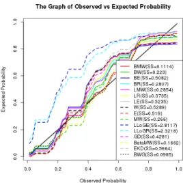
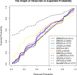
Plots of the fitted densities, the histogram of the data and probability plots by Cham-bers et al. (1983) are given in Figure 3, Figure 4, Figure 5 and Figure 6. For the proba-bility plot, we plotted F(y(j); ˆc,ˆk,α,ˆ β,ˆ λ) againstˆ

j−0.375

n+ 0.25, j = 1,2,· · · , n,where y(j) are the ordered values of the observed data. The measures of closeness are given by the sum of squares SS = n X j=1 F(y(j))− j−0.375 n+ 0.25 2 . 8.1 Aarset Data

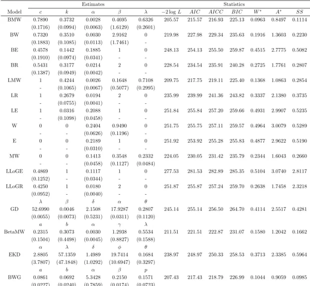
The data contains the times to failure of 50 devices put on life test at time 0, Aarset (1987). The parameter estimates, goodness-of-fit statistics and results for this data are given in Table 5. The estimated variance-covariance matrix for the BMW distribution is given by:

Table 5: Estimates of Models for Aarset Data

Estimates Statistics

Model c k α β λ −2 logL AIC AICC BIC W∗ _A∗ _SS

BMW 0.7890 0.3732 0.0028 0.4695 0.6326 205.57 215.57 216.93 225.13 0.0963 0.8497 0.1114 (0.1716) (0.0994) (0.0063) (1.6129) (0.2601) BW 0.7320 0.3510 0.0030 2.9162 0 219.98 227.98 229.34 235.63 0.1916 1.3603 0.2230 (0.1883) (0.1085) (0.0113) (1.7461) -BE 0.4578 0.1442 0.1885 1 0 248.13 254.13 255.50 259.87 0.4515 2.7775 0.5082 (0.1910) (0.0974) (0.0341) - -BR 0.5431 0.3177 0.0214 2 0 228.54 234.54 235.91 240.28 0.2725 1.7761 0.2807 (0.1387) (0.0949) (0.0042) - -LMW 1 0.4244 0.0026 0.1648 0.7108 209.75 217.75 219.11 225.40 0.1368 1.0863 0.2854 - (0.1065) (0.0067) (0.5077) (0.2995) LR 1 0.2679 0.0194 2 0 235.99 239.99 241.36 243.82 0.3337 2.1380 0.3735 - (0.0755) (0.0041) - -LE 1 0.0316 0.2088 1 0 251.84 255.84 257.20 259.66 0.4931 2.9907 0.5235 - (0.1098) (0.0458) - -W 0 0 0.2404 0.9490 0 251.75 255.75 257.11 259.57 0.4964 3.0079 0.5289 - - (0.0626) (0.1196) -E 0 0 0.2189 1 0 251.92 253.92 255.28 255.83 0.4877 2.9622 0.5190 - - (0.0310) - -MW 0 0 0.1413 0.3548 0.2332 224.05 230.05 231.42 235.79 0.2344 1.6043 0.2660 - - (0.0458) (0.1127) (0.0484) LLoGE 0.4869 1 0.1117 1 0 277.53 281.53 282.89 285.35 0.5104 3.0740 2.8117 (0.1252) - (0.0344) - -LLoGR 0.4250 1 0.0180 2 0 251.87 255.87 257.24 259.70 0.2638 1.7458 2.3218 (0.0952) - (0.0040) - -λ β δ α θ GD 52.6990 0.0046 2.1508 17.9287 0.2807 245.14 255.14 256.50 264.70 0.4114 2.5517 0.4281 (0.0055) (0.0073) (0.5231) (0.0311) (0.1120) a b α γ λ BetaMW 0.2315 0.3073 0.0030 1.2938 0.5534 211.51 221.51 222.87 231.07 0.1580 1.2042 0.1662 (0.1504) (0.4498) (0.0045) (0.8827) (0.1588) α λ δ φ θ EKD 2.8805 57.1359 1.4989 19.7414 0.1684 238.97 248.97 250.33 258.53 0.3713 2.3385 0.5964 (3.7807) (47.1848) (1.0292) (10.6947) (0.3297) a b α β p BWG 0.0861 0.0692 5.3428 0.2150 0.1571 207.43 217.43 218.79 226.99 0.1044 0.9059 0.0985 (0.0227) (0.0240) (0.7859) (0.0174) (0.0723)         0.0295 −0.0060 0.0000 −0.0277 0.0081 −0.0060 0.0099 −0.0002 0.0303 0.0003 0.0000 −0.0002 0.0000 −0.0080 0.0003 −0.0277 0.0303 −0.0080 2.6014 −0.3224 0.0081 0.0003 0.0003 −0.3224 0.0677         ,

and the 95% confidence intervals for the model parameters are given by c ∈(0.7890±

1.96×0.1716), k∈(0.3732±1.96×0.0994), α∈(0.0028±1.96×0.0063), β∈(0.4695±

1.96×1.6129) andλ∈(0.6326±1.96×0.2601),respectively.

The LRT statistic for testing H0: BW against Ha: BMW and H0: BR against Ha:

Figure 3: Fitted Densities for Aarset Data

Figure 4: Probability Plots for Aarset Data

conclude that there is a significant difference between the BW and the BMW distri-butions, and also between the BR and the BMW distributions. The LRT statistic for testingH0: LMW againstHa: BMW is 4.18 (p-value=0.0409<0.05). We conclude that there is a significant difference between the LMW and the BMW distribution at the 5% level. There is indeed clear and convincing evidence based on the goodness-of-fit statis-ticsW∗ and A∗ that the BMW distribution is far better than the sub-models, and the non-nested models. Also, the values of AIC and BIC shows that the BMW distribution is better than the non-nested GD, EKD, BetaMW and BWG distributions.

Table 6: Estimates of Models for Kevlar Failure Data

Estimates Statistics

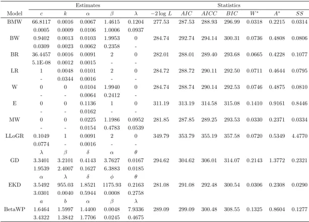
Model c k α β λ −2 logL AIC AICC BIC W∗ _A∗ _SS BMW 66.8117 0.0016 0.0067 1.4615 0.1204 277.53 287.53 288.93 296.99 0.0318 0.2215 0.0314 0.0005 0.0009 0.0106 1.0006 0.0937 BW 0.9402 0.0013 0.0103 1.9953 0 284.74 292.74 294.14 300.31 0.0736 0.4808 0.0806 0.0309 0.0023 0.0062 0.2358 -BR 36.4457 0.0016 0.0091 2 0 282.01 288.01 289.40 293.68 0.0665 0.4228 0.1077 5.1E-08 0.0012 0.0015 - -LR 1 0.0048 0.0101 2 0 284.72 288.72 290.11 292.50 0.0711 0.4644 0.0795 - 0.0344 0.0016 - -W 0 0 0.0104 1.9940 0 284.74 288.74 290.14 292.53 0.0746 0.4875 0.0810 - - 0.0064 0.2412 -E 0 0 0.1136 1 0 311.19 313.19 314.58 315.08 0.1410 0.9161 0.8446 - - 0.0162 - -MW 0 0 0.0225 1.1986 0.0952 281.85 287.85 289.25 293.53 0.0330 0.2371 0.0334 - - 0.0154 0.4783 0.0539 LLoGR 0.1049 1 0.0091 2 0 349.79 353.79 355.19 357.58 0.0720 0.5349 4.4770 0.0774 - 0.0016 - -λ β δ α θ GD 3.3401 3.2101 0.4143 3.7627 0.0167 294.62 304.62 306.01 314.07 0.2143 1.3772 0.2321 1.9539 2.4007 0.1627 6.3883 0.0185 α λ δ φ θ EKD 3.5492 955.03 1.8521 1175.93 0.2163 281.08 291.08 292.48 300.54 0.0306 0.2308 0.0290 3.0301 0.0040 0.5944 0.0008 0.2758 a b α β λ BetaWP 1.6464 1.5997 1.4400 0.0048 7.9336 289.09 299.09 300.48 308.55 0.1325 0.8604 0.1277 3.4322 1.3842 1.7706 0.0245 0.4675

8.2 Kevlar 49/Epoxy Strands Failure Data

The 49 data points represent the stress-rupture life of kevlar 49/epoxy strands which were subjected to constant sustained pressure at the 70% stress level until all had failed, as in the previous example, we have complete data with exact times of failure, Andrews and Herzberg (1985). The estimate results for this data is given in Table 6. The estimated variance-covariance matrix for the BMW distribution is given by:

       

2.3E−07 6.9E−08 −4.7E−06 4.8E−04 −4.0E−05 6.9E−08 7.8E−07 −3.5E−06 1.4E−04 5.9E−06

−4.7E−06 −3.5E−06 1.1E−04 −9.7E−03 6.4E−04 4.8E−04 1.4E−04 −9.7E−03 1.0E+ 00 −8.4E−02

−4.0E−05 5.9E−06 6.4E−04 −8.4E−02 8.8E−03

        ,

and the 95% confidence intervals for the model parameters are given by c∈(66.8117±

1.96×0.0005), k∈(0.0016±1.96×0.0009), α∈(0.0067±1.96×0.0106), β∈(1.4615±

1.96×1.0006) andλ∈(0.1204±1.96×0.0937),respectively.

The LRT statistic for testingH0: LR againstHa: BMW andH0: W againstHa: BMW

Figure 5: Fitted Densities for Kevlar Failure Data

Figure 6: Probability Plots for Kevlar Failure Data

that there is a significant difference between the LR and the BMW distributions, and also between the W and the BMW distributions at the 10% level. We conclude that there is a significant difference between the BW and the BMW distributions (LRT statistic ω= 7.21, p-value-0.00725). There is also a significant difference between the LLoGR and the BMW distributions based on the LRT. There is no significant difference between the MW and the BMW distributions based on the LRT, however, there is indeed clear and convincing evidence based on the goodness-of-fit statistics W∗ and A∗ that the BMW distribution is far better than the sub-models, and the non-nested models. Also, the

values of AIC and BIC shows that the BMW distribution is better than the sub-models and the non-nested GD, EKD, and BetaWP distributions.

9 Concluding Remarks

In this paper, a new distribution called Burr XII modified Weibull (BMW) distribu-tion was introduced. The statistical properties of the BMW distribudistribu-tion including the hazard and reverse hazard functions, quantile function, moments, incomplete moments, generating functions, mean deviations, Bonferroni and Lorenz curves, order statistics, R´enyi entropy and maximum likelihood estimation for the model parameters are given. Simulation studies was conducted to examine the performance of the new BMW distri-bution. We also presented applications of this new model to real life datasets in order to illustrate the usefulness of the distribution.

Acknowledgement

The authors would like to thank the editor and the referees for carefully reading the paper and for their valuable comments, which greatly improved the presentation of this paper.

References

Aarset, M. V. (1987). How to identify bathtub hazard rate. IEEE Transactions on Reliability, 36(1):106–108.

Andrews, D. F. and Herzberg, A. M. (1985). A Collection of Problems from Many Fields for the Students and Research Workers. Springer Series in Statistics, New York: Springer.

Barakat, H. M. and Abdelkader, Y. H. (2004). Computing the moments of order statistics from nonidentical random variables. Statistical Methodology and Applications, 13. Bidram, H., Behboodian, J., and Towhidi, M. (2013). The beta weibull geometric

dis-tribution. Journal of Statistical Computation and Simulation, 83(1):52–67.

Burr, I. W. (1942). Cumulative frequency functions.The Annals of Mathematical Statis-tics, 13(2):215232.

Burr, I. W. and Cislak, P. J. (1968). On a general system of distributions: I. its curve shaped characteristics, ii . the sample median. The Annals of Mathematical Statistics, 63:627–635.

Chambers, J., Cleveland, W., Kleiner, B., and Tukey, P. (1983). Graphical Methods of Data Analysis. Chapman and Hall.

Chen, G. and Balakrishnan, N. (1995). A general purpose approximate goodness-of-fit test. Journal of Quality Technology, 27:154–161.

Gurvich, M. R., DiBenedetto, A. T., and Ranade, S. V. (1997). A new statistical distribution for characterizing the random strength of brittle materials. Journal of Materials Science, 32:2559–2564.

Hatke, M. A. (1949). A certain cumulative probability function. The Annals of Mathe-matical Statistics, 20:461–463.

Hoskings, J. R. M. (1990). L-moments: Analysis and estimation of distributions using linear combinations of order statistics. Journal of the Royal Statistical Society, B 52:105–124.

Huang, S. and Oluyede, B. O. (2014). Exponentiated kumaraswamy-dagum distribution with applications to income and lifetime data. Journal of Statistical Distributions and Applications, 1(8).

Lai, C. D., Xie, M., and Murthy, D. N. P. (2003). A modified weibull distribution.IEEE Transactions on Reliability, 52(1):33–37.

Mudholkar, G. S. and Srivastava, D. K. (1993). Exponentiated weibull family for ana-lyzing bathtub failure-rate data. IEEE Transactions on Reliability, 42:299–302. Nadarajah, S., Cordeiro, G. M., and Ortega, E. M. M. (2011). General results for the

beta-modified weibull distribution. Journal of Statistical Computation and Simula-tions, 81(10):1211–1232.

Oluyede, B. O., Huang, S., and Pararai, M. (2014). A new class of generalized dagum distribution with applications to income and lifetime data. Journal of Statistical and Econometric Methods, 3(2):125–151.

Oluyede, B. O., Huang, S., and Yang, T. (2015). A new class of generalized modified weibull distribution with applications. Austrian Journal of Statistics, 44:45–68. Percontini, A., Blas, B., and Cordeiro, G. M. (2013). The beta weibull poisson

distribu-tion. Chilean Journal of Statistics, 4(2):3–26.

Pham, H. and Lai, C. D. (2007). On recent generalizations of the weibull distribution.

IEEE Transaction on Reliability, 56:454–458.

R´enyi, A. (1960). On measures of entropy and information. InProceedings of the Fourth Berkeley Symposium on Mathematical Statistics and Probability, volume 1, pages 547 – 561.

Rodrigues, R. N. (1977). A guide to the burr type xii distributions. Biometrika, 64:129– 134.

Santos Silva, J. M. and Tenreyro, S. (2010). On the existence of maximum likelihood estimates in poisson regression. Economics Letters, 107:310–312.

Seregin, A. (2010). Uniqueness of the maximum likelihood estimator for k-monotone densities. Proceedings of the American Mathematical Society, 138:4511–4515.

Soliman, A. A. (2005). Estimation of parameters of life from progressively censored data using burr-xii model. IEEE Transactions on Reliability, 54:34–42.

Tadikamalla, P. R. (1980). A look at the burr and related distributions. International Statistical Reviews, 48:337–344.

Foundation for Statistical Computing, Vienna, Austria.

Weibull, W. A. (1951). Statistical distribution function of wide applicability. Journal of Applied Mechanics, 18:293–296.

Xia, J., Mi, J., and Zhou, Y. Y. (2009). On the existence and uniqueness of the maximum likelihood estimators of normal and log-normal population parameters with grouped data. Journal of Probability and Statistics, Article id 310575:16 pages.

Zhou, C. (2009). Existence and consistency of the maximum likelihood estimator for the extreme index. Journal Multivariate Analysis, 100:794–815.

Appendix

R Algorithms

#### d e f i n e BMW p d f

BMW pdf=f u n c t i o n ( c , k , alpha , beta , lambda , x ){

(1+xˆ c )ˆ(−k−1)∗( exp(−a l p h a∗xˆ b e t a∗exp ( lambda∗x ) ) )∗

( k∗c∗x ˆ ( c−1)+(1+xˆ c )∗a l p h a∗exp ( lambda∗x )∗x ˆ ( beta−1)∗( b e t a+lambda∗x ) )

}

#### d e f i n e BMW c d f

BMW cdf=f u n c t i o n ( c , k , alpha , beta , lambda , x ){

1−(1+xˆ c )ˆ(−k )∗( exp(−a l p h a∗( xˆ b e t a )∗exp ( lambda∗x ) ) )

}

#### d e f i n e BMW q u a n t i l e

BMW quantile=f u n c t i o n ( c , k , alpha , beta , lambda , u ){

f=f u n c t i o n ( x ){ k∗l o g (1+xˆ c )+ a l p h a∗xˆ b e t a∗exp ( lambda∗x)+ l o g (1−u ) } x=u n i r o o t ( f , c ( 0 , 1 0 0 ) ) $ r o o t r e t u r n ( x ) } #### d e f i n e BMW h a z a r d

BMW hazard=f u n c t i o n ( y , c , k , alpha , beta , lambda ){

BMW pdf( y , c , k , alpha , beta , lambda )/(1−BMW cdf ( y , c , k , alpha , beta , lambda ) )

}

#### d e f i n e moments o f BMW

BMW moments=f u n c t i o n ( c , k , alpha , beta , lambda , r ){

f=f u n c t i o n ( y , c , k , alpha , beta , lambda , r ){

}

y=i n t e g r a t e ( f , l o w e r =0 , upper=I n f , s u b d i v i s i o n s =1000000 , c=c , k=k , a l p h a=alpha , b e t a=beta , lambda=lambda , r=r )

r e t u r n ( y $ v a l u e )

}

#### d e f i n e s i m u l a t i o n p r o c e s s o f BMW

BMW simulation=f u n c t i o n ( s i z e=c ( 2 5 , 5 0 , 1 0 0 , 2 0 0 , 4 0 0 , 8 0 0 ) , samp , p a r 1 ){

Mean=v e c t o r ( ) RMSE=v e c t o r ( ) B i a s=v e c t o r ( )

f o r ( i t e r s i z e i n 1 : l e n g t h ( s i z e ) ){

c o e f 1=m a t r i x (NA, samp , 5 )

c o l n a m e s ( c o e f 1 )= c ( ’ c ’ , ’ k ’ , ’ alpha ’ , ’ beta ’ , ’ lambda ’ ) f o r ( nsamp i n 1 : samp ){ t r y C a t c h ( { x1 BMW=NULL q=r u n i f ( s i z e [ i t e r s i z e ] , 0 , 1 ) x1=s a p p l y ( q , BMW quantile ,

c=p a r 1 [ 1 ] , k=p a r 1 [ 2 ] , a l p h a=p a r 1 [ 3 ] , b e t a=p a r 1 [ 4 ] , lambda=p a r 1 [ 5 ] ) ### BMW f o r x1

x1 BMW<−mle2 ( BMW neglogl ,

s t a r t= l i s t ( c=p a r 1 [ 1 ] , k=p a r 1 [ 2 ] , a l p h a=p a r 1 [ 3 ] , b e t a=p a r 1 [ 4 ] , lambda=p a r 1 [ 5 ] ) , method=”L−BFGS−B” , d a t a= l i s t ( x=x1 ) ,

l o w e r=c ( c =0 ,k=0 , a l p h a =0 , b e t a =0 , lambda =0) ,

upper=c ( c=I n f , k=I n f , a l p h a=I n f , b e t a=I n f , lambda=I n f ) , u s e . g i n v=TRUE) c o e f 1 [ nsamp , ] = c o e f (x1 BMW)

}, e r r o r=f u n c t i o n ( e ){ }

)

}

Mean [ l e n g t h ( s i z e )∗( 0 : 4 ) + i t e r s i z e ]= a p p l y ( c o e f 1 , 2 , mean , na . rm=TRUE)

RMSE[ l e n g t h ( s i z e )∗( 0 : 4 ) + i t e r s i z e ]= a p p l y ( ( c o e f 1−m a t r i x ( r e p ( par1 , nsamp ) , n c o l =5 , byrow=T) ) ˆ 2 , 2 , f u n c t i o n ( x ){s q r t ( mean ( x , na . rm=TRUE) )})

}

B i a s=a s . v e c t o r ( s a p p l y ( 1 : 5 , f u n c t i o n ( x ){B i a s [ ( l e n g t h ( s i z e )∗( x−1)+1):

( l e n g t h ( s i z e )∗x ) ] =Mean [ ( l e n g t h ( s i z e )∗( x−1 ) + 1 ): ( l e n g t h ( s i z e )∗x )]−p a r 1 [ x ]}) ) s a m p l e s i z e=a s . v e c t o r ( t ( mapply ( rep , s i z e , 5 ) ) )

r e t u r n ( c b i n d ( s a m p l e s i z e , Mean ,RMSE, B i a s ) )

}

# f u n c i t o n t o c a l c u l a t e Cramer−von and Anderson−D a r l i n g s t a t i s t i c s WABMW=f u n c t i o n ( f i t , x , s i g n ){

u=g e t ( p a s t e 0 ( s i g n , ’ c d f ’ ) ) ( c o e f ( f i t ) [ 1 ] , c o e f ( f i t ) [ 2 ] , c o e f ( f i t ) [ 3 ] , c o e f ( f i t ) [ 4 ] , c o e f ( f i t ) [ 5 ] , x ) } e l s e{ u=BMW cdf ( c o e f ( f i t ) [ 1 ] , c o e f ( f i t ) [ 2 ] , c o e f ( f i t ) [ 3 ] , c o e f ( f i t ) [ 4 ] , c o e f ( f i t ) [ 5 ] , x ) } y=qnorm ( u )

v=pnorm ( ( y−mean ( y ) ) / ( a s . numeric ( s q r t ( v a r ( y ) ) ) ) )

W2=sum ( ( v−((2∗s e q ( 1 , l e n g t h ( x ) )−1 ) / ( 2∗l e n g t h ( x ) ) ) ) ˆ 2 ) + 1 / ( 1 2∗l e n g t h ( x ) ) A2=−l e n g t h ( x)−sum ( ( ( 2∗s e q ( 1 , l e n g t h ( x ) )−1 )∗( l o g ( v ) ) ) + ( ( 2∗l e n g t h ( x)+1−2∗s e q ( 1 , l e n g t h ( x ) ) )∗( l o g (1−v ) ) ) ) / l e n g t h ( x ) W=W2∗( 1 + 0 . 5 / l e n g t h ( x ) ) A=A2∗( 1 + 0 . 7 5 / l e n g t h ( x ) + 2 . 2 5 / l e n g t h ( x ) / l e n g t h ( x ) ) r e s u l t= l i s t (W=W,A=A) r e t u r n ( r e s u l t ) } # d e f i n e t h e f u n c t i o n t o c a l c u l a t e SS v a l u e SS BMW=f u n c t i o n ( f i t , x , s i g n ){ pp=( s e q ( 1 , l e n g t h ( x ) , 1 )−0 . 3 7 5 ) / ( l e n g t h ( x ) + 0 . 2 5 ) i f ( ! i s . n u l l ( g e t 0 ( p a s t e 0 ( s i g n , ’ c d f ’ ) ) ) ){ op=g e t ( p a s t e 0 ( s i g n , ’ c d f ’ ) ) ( c o e f ( f i t ) [ 1 ] , c o e f ( f i t ) [ 2 ] , c o e f ( f i t ) [ 3 ] , c o e f ( f i t ) [ 4 ] , c o e f ( f i t ) [ 5 ] , s o r t ( x ) ) } e l s e{ op=BMW cdf ( c o e f ( f i t ) [ 1 ] , c o e f ( f i t ) [ 2 ] , c o e f ( f i t ) [ 3 ] , c o e f ( f i t ) [ 4 ] , c o e f ( f i t ) [ 5 ] , s o r t ( x ) ) } SS=0 f o r ( i i n 1 : l e n g t h ( x ) ){ SS=SS+(op [ i ]−pp [ i ] ) ˆ 2 } r e s u l t= l i s t ( pp=pp , op=op , SS=SS ) r e t u r n ( r e s u l t ) } # BMW F i t

mysample BMW<−mle2 ( BMW neglogl ,

s t a r t= l i s t ( c =1 ,k=1 , a l p h a =1 , b e t a =1 , lambda =1) , method=”L−BFGS−B” , d a t a= l i s t ( x=mysample ) , l o w e r=c ( c =0 ,k=0 , a l p h a =0 , b e t a =0 , lambda =0) ,