An Approach to a Hybrid Software Process Simulation using the DEVS Formalism

(www.interscience.wiley.com) DOI: 10.1002/spip.284

An Approach to a Hybrid

Software Process

Simulation using the DEVS

Formalism

Research Section

KeungSik Choi,*

_{Doo-Hwan Bae and TagGon Kim}

Department of EECS, Korea Advanced Institute of Science and Technology (KAIST), Daejon 305-701, Korea

This article proposes an approach to a hybrid software process simulation modeling (SPSM)

using discrete event system specification (DEVS) formalism, which implements the dynamic

structure and discrete characteristics of the software development process. Many previous

researchers on hybrid SPSM have described both discrete and continuous aspects of the

software development process to provide more realistic simulation models. The existing hybrid

models, however, have not fully implemented the feedback loop mechanism of the system

dynamics.

We define the DEVS Hybrid SPSM formalism by extending DEVS to the hybrid SPSM domain.

Our hybrid SPSM approach uses system dynamics modeling to convey details concerning

activity behaviors and managerial policies, while discrete event modeling controls activity

start/completion and sequence. This approach also provides a clear specification, an explicit

extension point to extend the simulation model, and a reuse mechanism. We will demonstrate

a Waterfall-like hybrid software process simulation model using the DEVS Hybrid SPSM

formalism. Copyright



2006 John Wiley & Sons, Ltd.

KEY WORDS: hybrid software process simulation modeling; DEVS formalism; model extension

1. INTRODUCTION

The software process shows both discrete system aspects (start/end of an activity and recep-tion/release of an artifact by an activity) and contin-uous system ones (percentage of developed prod-uct, percentage of discovered defects) (Donzelli and Iazeolla 2001). In other words, the software process is composed of event-driven dynamics (artifacts

∗_{Correspondence to: KeungSik Choi, Department of EECS,}

Korea Advanced Institute of Science and Technology (KAIST), Daejon 305-701, Korea

†_{E-mail: [email protected]}

Copyright2006 John Wiley & Sons, Ltd.

moving among different activities, phase transi-tion) and time-driven dynamics (dynamic behavior by the feedback structure of the process). Discrete event models describe the software development process as a sequence of discrete activities, and rep-resent the process details, such as code complexity and programmer capability, through the attributes of each entity, but may not have enough events to represent the continuously varying dynamics of the process. On the other hand, the system dynamics models describe the interactions between project factors, but do not easily represent discrete process steps (Martin and Raffo 2000).

Many researchers have tried to combine discrete event simulation and continuous simulation to

model software processes more realistically. Rus

et al. (1999) and Lakey (2003) made it possible to explicitly analyze the performance of each discrete process while incorporating the feedback loop mechanism. Martin and Raffo (2000) analyzed the manpower utilization using a hybrid simulation model, which shows us how manpower levels vary on the basis of the changes in workforce, hiring delays, allocation decisions, and the point at which the available manpower is wasted. This analysis is not reproducible in the continuous or discrete model alone. Donzelli and Iazeolla (2001) combined the three traditional modeling methods (analytical, continuous, and discrete event).

The previous researchers, however, have not fully represented the feedback loop mechanism of the system dynamics. The feedback loops approxi-mated by Ruset al. (1999) and Lakey (2003) are too coarse to fully represent the dynamics of continu-ously interacting variables such as schedule, size, quality, manpower, overhead, skill level, etc. Mar-tin and Raffo (2000) assumed that the workload for an activity is constant during its life-cycle, which prevents the model from calculating the activity duration dynamically. This affects all the dynamics of the combined model. Donzelli and Iazeolla (2001) have not explicitly represented the managerial con-trols, such as schedule pressure, fatigue, training policies, and staff experience, that are incorporated in the feedback loops of system dynamics.

We propose a DEVS-based hybrid software pro-cess simulation modeling (SPSM) method, which fully represents the feedback mechanism of sys-tem dynamics and the discrete phase transition. We define DEVS Hybrid SPSM formalism by extend-ing DEVS (discrete event system specification) to the hybrid SPSM domain. Our hybrid SPSM approach uses the system dynamics modeling to convey details concerning the activity behaviors and man-agerial policies, while the discrete event modeling controls the activity start/completion and sequence. This approach also provides a clear specification, an explicit extension point to extend the simulation model, and a reuse mechanism.

The structure of this article is as follows. In Section 2 we compare and analyze the pub-lished hybrid SPSM approaches. Section 3 intro-duces the characteristics of the DEVS-based hybrid SPSM approach. It describes the concept of for-malism embedding and the characteristics of

DEVS Hybrid SPSM formalism, which is an exten-sion of DEVS formalism to the hybrid software process simulation. Section 4 shows the overall architecture of the Waterfall-like life-cycle model as a case study and analyzes the simulation result with different normal productivity values for each phase. Section 5 summarizes the main results of this article and gives a plan for future work.

2. ANALYSIS OF THE PUBLISHED HYBRID

SPSM APPROACHES

2.1. Detailed Analysis on the Existing Hybrid SPSM Approaches

Ruset al. (1999) and Lakey (2003) represent the pro-cess as discrete activities and try to incorporate the feedback loops of system dynamics. They incorpo-rate feedback loops by dividing the inputs by five, iterating five times, calculating product, process, and project factors, and passing the attributes on to the next activity. One of the advantages of this approach is that it is possible to explicitly analyze the performance of each discrete process, which is regarded as a difficult task in system dynamics simulation (Martin and Raffo 2000).

This approach, however, approximates the sys-tem dynamics models too coarsely and does not include the managerial aspect of the software pro-cess, such as decision rules for manpower allocation, scheduling, etc. Furthermore, the feedback mecha-nism of this approach is different from the basic principle of system dynamics. The behavior of a system is derived from the structure of the feedback loops and the stocks and flows in system dynam-ics (Sterman 2004), but this approach calculates the dynamic variables as the product of several param-eters as shown in Equation (1). The paramparam-eters are used to offset the estimated values of the process (Lakey 2003). TheSchedule, Size, andQualityfactors are calculated and updated during each of the five iterations, but the remaining factors are static.

DevelopEffort=ExpectedDevelopEffort×Schedule

×Size×Quality×Manpower×Overhead

×Skill×ToolSupport×Maturity×Growth (1) Martin and Raffo (2000) have developed a hybrid simulation model, which ensures that the discrete activities are consistent with the implied activities Copyright2006 John Wiley & Sons, Ltd. Softw. Process Improve. Pract., 2006; : 373–383

of the continuous portion. This combined model would allow investigation of the effects of discrete resource changes on continuously varying produc-tivity and the influences of the duration of discrete code inspection tasks on continuously changing error rates. This is a creative way of combining discrete event and system dynamics paradigm.

However, this approach has similar problems as the approach of Ruset al. and Lakey. The estimated required workload is constant during the life-cycle, so it does not represent the feedback structure properly. The workload may increase because of the reworks, which dynamically affect the activity duration.

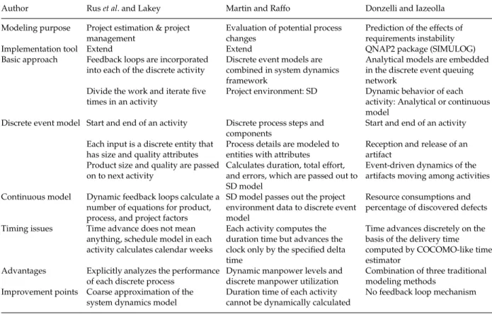
Donzelli and Iazeolla (2001) combine three tra-ditional modeling methods, which are analytical, continuous, and discrete modeling, but they do not explicitly represent the feedback loop mechanism of system dynamics and the managerial controls, such as schedule pressure, fatigue, training policies, and staff experience. You can refer the detailed descrip-tions in the proceedings of the ProSim’05 (Choiet al. 2005). Table 1 describes and compares the discussed hybrid SPSM approaches.

2.2. Results of the Analysis

Through the analysis of previous research we asked what needed to be continuous and what needed to be discrete in software process simulation models and what we needed to know about the process in order to use the hybrid model. Of course, these depend on the purpose of the simulation modeling, but we examined the aspects that are most appropriate for general software process simulation models.

We concluded that the hybrid software process simulation model should be a discrete model in phase (activity) transition (e.g. from Requirements to Design), and a system dynamics model not only within the activity but also in the overall process life-cycle. By taking advantage of previous research and incorporating the ‘Improvement points’ (Table 1) we defined the functionalities of the hybrid software process simulation models as follows:

• Fully incorporating the feedback mechanism of the system dynamics.

• Analyzing the performance of each discrete process explicitly.

• Making the discrete activities consistent with the activities of the continuously varying project environments.

3. AN APPROACH TO A HYBRID

SOFTWARE PROCESS SIMULATION USING

DEVS FORMALISM

We have extended the DEVS formalism to apply it to hybrid SPSM because DEVS is a general, extensible, and easily verifiable formalism. It also has several simulation engines in public domain, which imple-ment the DEVS formalism. The extended formalism provides natural hybrid simulation modeling capa-bilities by enabling both discrete and continuous simulation modeling in the same environment and also provides the defined functionalities for the hybrid software process simulation model.

3.1. DEVS Formalism

DEVS is a general formalism for discrete event sys-tem modeling based on set theory (Zeigler et al. 2000). It allows representing any system by three sets and four functions: input set, output set, state set, external transition function, internal transition function, output function, and time advanced func-tion. DEVS formalism provides the framework for information modeling, which has several advan-tages, such as completeness, verifiability, extensibil-ity, and maintainability (Kim 2004), for analyzing and designing complex systems. DEVS can also approximate continuous systems using numerical integration methods. Thus, simulation tools based on DEVS are potentially more general than other tools, including continuous simulation tools (Kof-manet al. 2003). With these properties, we applied DEVS formalism to the hybrid SPSM.

DEVS has two kinds of models to represent systems. One is an atomic model and the other is a coupled model that can specify complex systems in a hierarchical way (Zeigleret al. 2000). The DEVS model processes an input event on the basis of its state and condition, and it generates an output event and changes its state. Finally, it sets the time during which the model can stay in that state. An atomic DEVS model is defined by the following structure (Zeigleret al. 2000):

M= X, Y, S, δext, δint, λ,ta,

Table 1. Comparison of the hybrid simulation modeling approaches

Author Ruset al. and Lakey Martin and Raffo Donzelli and Iazeolla Modeling purpose Project estimation & project

management

Evaluation of potential process changes

Prediction of the effects of requirements instability

Implementation tool Extend Extend QNAP2 package (SIMULOG)

Basic approach Feedback loops are incorporated into each of the discrete activity

Discrete event models are combined in system dynamics framework

Analytical models are embedded in the discrete event queuing network

Divide the work and iterate five times in an activity

Project environment: SD Dynamic behavior of each activity: Analytical or continuous model

Discrete event model Start and end of an activity Discrete process steps and components

Start and end of an activity Each input is a discrete entity that

has size and quality attributes

Process details are modeled to entities with attributes

Reception and release of an artifact

Product size and quality are passed on to next activity

Calculates duration, total effort, and errors, which are passed out to SD model

Event-driven dynamics of the artifacts moving among activities Continuous model Dynamic feedback loops calculate a

number of equations for product, process, and project factors

SD model passes out the project environment data to discrete event model

Resource consumptions and percentage of discovered defects Timing issues Time advance does not mean

anything, schedule model in each activity calculates calendar weeks

Each activity computes the duration time but advances the clock only by the specified delta time

Time advances discretely on the basis of the delivery time computed by COCOMO-like time estimator

Advantages Explicitly analyzes the performance of each discrete process

Dynamic manpower levels and discrete manpower utilization

Combination of three traditional modeling methods

Improvement points Coarse approximation of the system dynamics model

Duration time of each activity cannot be dynamically calculated

No feedback loop mechanism

where

• X is the set of input values,

• Y is the set of output values,

• S is the set of states,

• δext: Q×X→S is the external transition

func-tion, where Q= {(s,e)|s∈S,0≤e≤ta(s)}is the total state set, e is the time elapsed since last transition,

• δint: S→S is the internal transition function,

• λ: S→Y is the output function,

• ta: S→R+0,∞ is the set positive real numbers between 0 and∞.

The DEVS coupled model is constructed by cou-pling the DEVS models. Through the coucou-pling, output events of one model are converted into input events of the other. In DEVS theory, the coupling of DEVS models defines new DEVS models (i.e. DEVS is closed under coupling) and complex systems can then be represented by DEVS in a hierarchical way (Zeigleret al. 2000).

3.2. Simulation Environment

The DEVSim++(Kim 2004) is a DEVS simulation environment based on C++, which is integrated with the Microsoft Visual Studio.NET. It therefore provides the advantages of object-oriented frame-work, such as encapsulation, inheritance, and reuse. The DEVSim++coordinates the event schedules of atomic models in a system and provides classes and APIs for simulation.

We get several advantages with DEVS formalism and DEVSim++. First, we can specify the sys-tems mathematically and easily verify the model. Second, we can model hierarchical and modu-larized systems, which enhance understandability and extensibility. Third, we can reuse simulation models.

3.3. Naturally Hybrid SPSM Environment using Formalism Embedding

Traditionally, differential equations have been solved with numerical integration in discrete time. Copyright2006 John Wiley & Sons, Ltd. Softw. Process Improve. Pract., 2006; : 373–383

In formal terms, differential equation system spec-ification (DESS) has been embedded into the dis-crete time system specification (DTSS) (Zeigleret al. 2000). The meaning of ‘embedded’ in this context is that any system in DESS can be simulated by DTSS. Of course, errors may be introduced in the DTSS approximation of the DESS model, but it is tolerable if the discrete time is small enough. Moreover, any DTSS can be simulated by the DEVS by constrain-ing the time advance to be constant. Therefore, if we constrain the time advance of the DEVS to be a small enough constant-time, we can model DESS with DEVS formalism. This formalism embedding makes DEVS-based hybrid SPSM technique to be a naturally hybrid simulation modeling approach. We coined the term ‘naturally hybrid’ because the formalism embedding provides both discrete and continuous simulation modeling capabilities in the same environment.

3.4. DEVS Hybrid SPSM: Hybrid SPSM Formalism

In this section we define the hybrid simula-tion modeling formalism for software process using formalism embedding, which is called DEVS Hybrid SPSM. We reference the discrete event and differential equation specified system (DEV&DESS) formalism (Zeigler et al. 2000) and extend the DEVS formalism to accommodate the hybrid characteristics of the software development process.

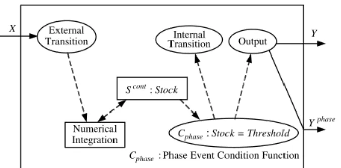
Figure 1 illustrates the modeling concept of the DEVS Hybrid SPSM, which embeds the DESS and DTSS formalism into DEVS. Input port of X accepts event segments, which are piecewise constant segments for numerical integration (Sterman 2004). The input message contains the flow (rate) and

Stock Scont: phase Y X Numerical Integration External

Transition _TransitionInternal Output Y

: phase C

phase

C :Stock =Threshold Phase Event Condition Function

Figure 1. The working mechanism of DEVS Hybrid SPSM formalism

stock variables, which are the output event message of the previous model. The continuous state, Scont, represents the stock variable of the system dynamics, which is used in the phase event condition function to determine the execution of the phase event. With input (X), output (Y), and continuous state (Scont), the atomic model implements the Euler integration (Sterman 2004) shown in Equation (2), which is driven by a small enough constant-time interval.

Scont

t+dt =S

cont

t +dt×(Xt−Yt) (2) The phase output event of Yphase occurs whenever a phase event condition function, Cphase, becomes

true. The condition can be observed when a certain software development activity reaches and crosses a predefined threshold (e.g. if 95% of preliminary design is completed, then the detailed design can be started). In such conditions, a phase event,

Yphase, is triggered, which contrasts with the time

events of pure DEVS in that the time events are scheduled by the time advance function. We define the DEVS Hybrid SPSM formalism as follows: DEVS Hybrid SPSM= X,Y,Yphase_{,S, δ}

ext, δint,

Cphase, λ,ta,

where

• X is the set of input values, which include flow (rate) vectors,

• Y is the set of output values, which include flow (rate) vectors,

• Yphase _{is the set of output values, which is the}

phase event triggered by phase event condition function (Cphase),

• S=Sdiscr×Scontis the set of states as a Cartesian

product of discrete states and continuous states,

• δext: Q×X→S is the external transition

func-tion where Q= {(sdiscr_,scont_,e)|_sdiscr∈_Sdiscr_,

scont∈

Scont,0≤e≤ta(s)}is the total state set, e is the time elapsed since last transition,

• δint: S→S is the internal transition function,

• Cphase: Q×X→Bool is the phase event

condi-tion funccondi-tion for condicondi-tioning the execucondi-tion of the phase event,

• λ: S→Y or Yphaseis the output function,

• ta: S→R+0,∞ is the set positive real number

between 0 and∞.

SD Model

Requirements Design Implementation Test Phase

Event

Hybrid software process simulation modeling using DEVS_Hybrid_SPSM (Naturally hybrid simulation modeling approach)

SD Model SD Model SD Model Phase Event Phase Event Phase Event Preliminary Design Detailed Design Test Feedback loop approximation: 5-times iterations

Rus and Lakey's approach DES Framework Discrete Process HR _{MP Alloc} Plan QA SD Framework

Martin and Raffo's approach

DES

Figure 2. Characteristics of DEVS Hybrid SPSM approach

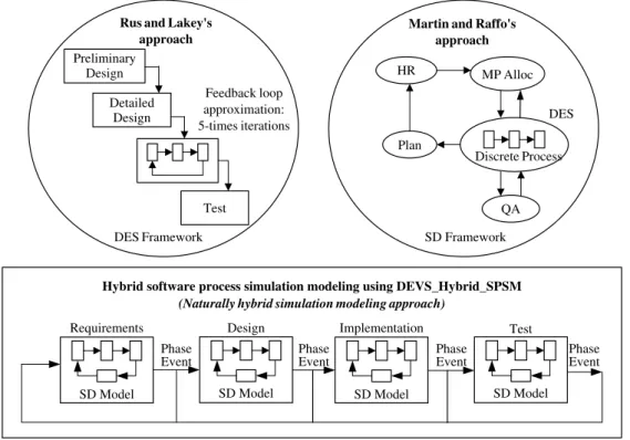
3.5. Characteristics of the DEVS Hybrid SPSM

Figure 2 illustrates the characteristics of the DEVS Hybrid SPSM approach compared with the pre-vious approaches. Rus and Lakey’s approach is fundamentally a discrete event simulation model and iterates multiple times within a discrete activ-ity to incorporate the feedback loops, but it might not fully represent the feedback loop mechanism and managerial aspect of the software process. This approach calculates process factors (e.g. effort, defects, and schedule) by the product of multiple factors (e.g. Equation (1)), and some of the fac-tors are constant. This cannot fully represent the dynamic behavior of a software development pro-cess that is represented in stock and flow concept and in which the process factors are calculated in the differential equation in the system dynamics model.

Martin and Raffo’s approach is fundamentally a system dynamics model of Abdel-Hamid and Madnick (1991). The continuously varying project variables (i.e. allocated manpower levels) are passed to the discrete process model (ISPW-6 process example (Kellner et al. 1991)) and the total effort

and errors are passed out to the system dynamics portion of the model. However, this approach might not calculate the activity duration dynamically.

In our DEVS Hybrid SPSM approach, each phase (e.g. requirements) by itself is a system dynamics model and the discrete phase transition explicitly occurs by the phase event, which transmits all the necessary dynamic variables through the event message to the next phase. The message, which is predefined, updates all the variables in the next phase model and collects the simulation data in the phase. Therefore, this approach can represent the discrete activities explicitly and consistently with the continuously varying project environments by fully incorporating the feedback mechanism of the system dynamics. This approach can also analyze the performance of each discrete process explicitly by capturing the phase output message.

Other advantages of this approach are that it provides a modularized and extensible simulation modeling environment. We modularize the simu-lation model by encapsulating closely related vari-ables in one atomic model and hide the complexity of the simulation model from the end user by pro-viding explicit interface for the simulation model. Copyright2006 John Wiley & Sons, Ltd. Softw. Process Improve. Pract., 2006; : 373–383

We also provide the explicit extension point through input and output ports. If any model has a compati-ble input or output port, the model can be extended. We can also reuse the simulation model by using the inheritance mechanism of the object-oriented framework of the DEVSim++environment.

4. CASE STUDY: IMPLEMENTING

WATERFALL-LIKE HYBRID SOFTWARE

PROCESS SIMULATION MODEL USING

THE DEVS HYBRID SPSM

This section describes how to model a

software development process using the

DEVS Hybrid SPSM formalism. We have devel-oped a generic building block for the develop-ment phase (activity) and impledevelop-ment a Waterfall-like hybrid software process simulation model by extending the generic building block. We have referenced and used the equations of the system dynamics models provided by Vensim simulation tool (Vensim 2004) and Abdel-Hamid and Madnick (1991). You can refer the detailed procedure for developing the hybrid software process simulation

model using DEVS Hybrid SPSM in the literature (Choiet al. 2005). The objectives of this case study are to provide the validation of this approach and to introduce a new method to model and analyze the software process more realistically.

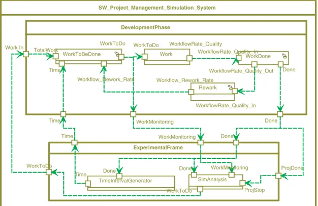
4.1. Architecture of the Generic Building Block

Figure 3 shows the overall architecture of the generic building block, which is composed of a ‘DevelopmentPhase’ and an ‘ExperimentalFrame’ model. It shows the most basic structure of the software development project. The ‘Development-Phase’ model represents any phase of the software development life-cycle, such as requirements, and can be extended to a Waterfall or Incremental life-cycle by coupling the ‘DevelopmentPhase’ model to each other through the explicit extension point (e.g. input or output port such as ‘Time’, ‘WorkMoni-toring’, and ‘Done’). The ‘WorkToBeDone’ model stores the amount of work to be done and sends it to the ‘Work’ model. The ‘Work’ model contains several submodels that calculate work flow, quality, etc. The ‘WorkDone’ model integrates the workflow rate to compute the work done, and the ‘Rework’

SW_Project_Management_Simulation_System WorkDone WorkflowRate_Quality_Out WorkflowRate_Quality_In Done Work WorkToDo WorkflowRate_Quality SimAnalysis Done WorkToDo ProjStop Rework Workflow_Rework_Rate WorkflowRate_Quality_In WorkToBeDone TotalWork Time WorkToDo TimeIntervalGenerator Done Time ExperimentalFrame Done ProjDone WorkMonitoring Time DevelopmentPhase Done WorkMonitoring Time Work In Workflow_Rework_Rate WorkToDo _{WorkMonitoring}

Figure 3. Overall architecture of a generic building block of DEVS-based SPSM

model computes the amount of rework to be done and sends the rework rate to the ‘WorkToBeDone’ model.

The ‘ExperimentalFrame’ model plays the role of a measurement system or observer, like an oscilloscope in Electronics. It generates an input to the observed system and accepts and analyzes the simulation data. In this simulation model it generates the ‘WorkToDo’ message, which is the initial work to be done. The ‘WorkToDo’ mes-sage will be processed by the ‘DevelopmentPhase’ model and it sends the simulation data, as a ‘Work-Monitoring’ message, to the ‘ExperimentalFrame’ model.

The ‘TimeIntervalGenerator’ model in the ‘Exper-imentalFrame’ is an executive that drives the simu-lation execution. It generates a Time event in a small enough constant-time interval to make the ‘Work-ToBeDone’ model change its state and generate the ‘WorkToDo’ message. The ‘TimeIntervalGenerator’ model enables the project variables to dynami-cally interact with each other, which allows this model to become a naturally hybrid simulation model.

All messages in this model include stock (level) variables, flow (rate) variables, and auxiliary vari-ables in system dynamics representation, which are dynamically updated through the feedback loop. The ‘WorkMonitoring’ message contains simula-tion status variables that are stored and analyzed

by the ‘SimAnalysis’ model in the ‘Experimental-Frame’ model. The ‘Done’ message generated by the ‘WorkDone’ model makes this simulation model stop.

4.2. Extending the Waterfall-like Software Process Simulation Model

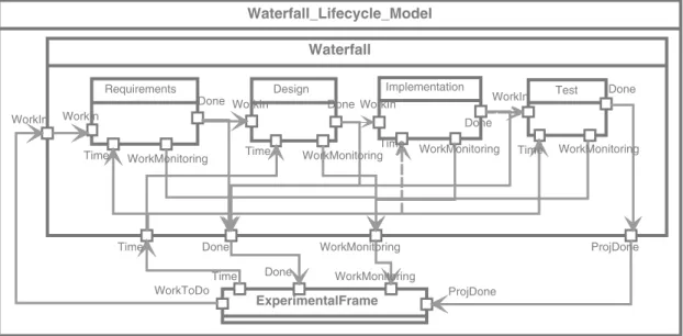
Figure 4 shows the Waterfall-like life-cycle model that is extended by coupling the ‘Development-Phase’ model to each other. The ‘Waterfall’ model starts when it receives ‘WorkIn’ input and ends when it receives the ‘ProjDone’ message. The ‘Requirements’ model performs the job and out-puts the ‘Done’ message when it completes the job. This message contains all the dynamic variables in the Requirements phase and transmits the infor-mation to the Design phase. The ‘WorkMonitoring’ message of each phase is sent to the ‘Experimen-talFrame’ model, which analyzes the performance of each discrete process explicitly. This model fully incorporates the feedback mechanism of the system dynamics and makes the discrete activities consis-tent with the activities of the continuously varying project environment variables.

Table 2 shows the specification of the ‘WorkDone’ model in the requirements phase, which generates the phase event when the requirements activity is more than 95% complete. This makes it explicit and easy to control the process sequencing.

Waterfall_Lifecycle_Model Test WorkIn Done WorkMonitoring Design WorkMonitoring WorkIn Time Done Implementation WorkIn Done WorkMonitoring Time ExperimentalFrame Done _{WorkMonitoring} Time ProjDone WorkToDo Requirements Done Waterfall ProjDone Done WorkIn Time WorkMonitoring WorkIn

Time _{WorkMonitoring} Time

Figure 4. Extended model: waterfall model

Table 2. DEVS Hybrid SPSM specification of the WorkDone model

WorkDone= X,Y,Yphase_{,S, δ}

ext, δint,Cphase, λ,ta

X= {WorkflowRate Quality In} Y= {WorkflowRate Quality Out} Yphase_{= {Requirements Done}}

S=WorkDone Discr×WorkDone Percent;

WorkDone Discr= {Wait, AccumulateWorkDone, Done, Stop}, WorkDone Percent=[0,100]

δext((Wait, WorkDone Percent), WorkflowRate Quality In)=

(AccumulateWorkDone, WorkDone Percent)

δint((AccumulateWorkDone, WorkDone Percent))=(Wait,

WorkDone Percent)

δint((Done, WorkDone Percent))=(Wait, WorkDone Percent)

Cphase(100.0>WorkDone Percent≥95.0); S=(Done,

WorkDone Percent)

Cphase(WorkDone Percent=100.0); S=(Stop,

WorkDone Percent)

λ((AccumulateWorkDone, WorkDone Percent))=λ((Done, WorkDone Percent))=WorkflowRate Quality Out

ta((Wait, WorkDone Percent))=ta((Stop, WorkDone Percent))

=Infinity

ta((AccumulateWorkDone, WorkDone Percent)=ta((Done, WorkDone Percent)=0

4.3. Simulation Results Analysis

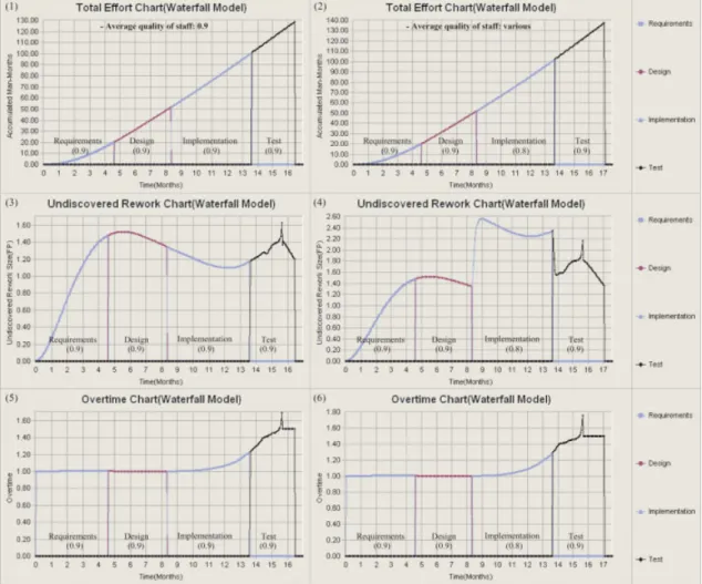
The implemented simulation model, which is available for research purposes in the author’s site (http://se.kaist.ac.kr/∼kschoi/DEVS Hybrid SPSM/), estimates the cost (Person-Month) and duration (Month) of a project using the initially estimated project size and duration. We can also set the variables, such as the average productivity and average quality of staffs, for each phase with different values, which makes this approach more realistic than others. In most previous research the variables are constant through the development cycle, which means that it is difficult to include the characteristics of each discrete activity explicitly in the simulation model. The developed simulation model allows various estimations and analyses during the development period through various charts, such as the accumulated project effort chart, undiscovered rework chart, and overtime chart, as shown in Figure 5.

Figure 5 shows the effects of the difference in the quality of individual staff in each discrete phase. It is valuable for planning and controlling the project to be able to predict the effort and duration of each phase when the average quality of staff planned to be assigned to each phase is variable. The factors affecting the error generation rate in a software project can be categorized into two: organization’s

factors (e.g. quality of staff and level of technique) and project factors (e.g. complexity, size of system, language) (Abdel-Hamid and Madnick 1991). In most previous research, the error generation rate is dependent on the percentage of the job completed or amount of overtime. They, however, have not taken into account the variable quality of the staff in each phase, to the best of my knowledge.

Chart (1) in Figure 5 shows the result when the average quality of staff throughout the development cycle is 0.9, which means that 10% of the completed job by the staff is erroneous. The accumulated total effort of Chart (1) is 128.8 (Person-Month) and the duration is 16.4 (Month). Chart (2) shows that the effort and duration are increased to 137.7 (Person-Month) and 17.1 ((Person-Month) because the average quality of staff in the implementation phase is lowered from 0.9 to 0.8.

Chart (3) in Figure 5 shows the amount of undis-covered rework (errors) in each phase when the average quality of staff throughout the develop-ment cycle is 0.9, and Chart (4) shows the amount of undiscovered rework in each phase when the aver-age quality of staff in the implementation phase is 0.8 and in the other phases is 0.9. Chart (4) implies that the undiscovered rework of the implementa-tion phase is increased owing to the lower average quality of staff, which causes the cost and duration to increase. We have run the simulation to find out the phase that is most sensitive for the lower average quality of staff. To do so, we changed the average quality of staff in the phases, one at a time, to 0.8 instead of 0.9. Table 3 shows that the implementa-tion phase influences the project cost and effort the most.

Chart (5) and (6) show the increase in the over-time by changing the average quality of the staff in the implementation phase from 0.9 to 0.8. The scale of the overtime, for instance 1.1, means that the working time of a staff is 10% more than the reg-ular working time of the organization. In Chart (6), the amount of overtime in the implementation and test phase is increased because the work size is increased as the project deadline is imminent.

This simulation run assumes that the resource is not constrained. We can extend this simu-lation model to include the resource constraint situation by adding a resource pool model that allocates the manpower when each phase sends a resource request event message. This extension Copyright2006 John Wiley & Sons, Ltd. Softw. Process Improve. Pract., 2006; : 373–383

Figure 5. Simulation results analysis charts: average quality of staff in all the phases shown in (1), (3), and (5) is 0.9, average quality of staff in the implementation phase shown in (2), (4), and (6) is 0.8

Table 3. Influences of the average quality of staff in each phase Average quality of staff

(default: 0.9) Normal (0.9) Requirements (0.8) Design (0.8) Implementation (0.8) Test (0.8)

Total effort (person-month) 128.8 130.9 132.6 137.7 134

Duration (month) 16.4 16.4 16.5 17.1 16.9

might provide a detailed analysis capability on the resource allocation policy.

5. CONCLUSION AND FUTURE WORK

feedback structure of the system dynamics, which was partially fulfilled in previous research, and explicitly represents the discrete activities, which enables us to analyze the performance of not only the overall process but also the discrete activities. This approach also provides clear specifications for model verification, explicit extension points to extend the model, and reuse mechanisms. We have also shown the applicability of our approach with the example of Waterfall-like life-cycle model. Copyright2006 John Wiley & Sons, Ltd. Softw. Process Improve. Pract., 2006; : 373–383

The simulation model provides powerful analysis capabilities that are not available in the discrete or continuous model alone and even in the existing hybrid approaches.

However, our approach has some limitations at this point because it is difficult to understand the formalism for industrial practitioners, and the case study described is not enough to show all the benefits of our approach. We, therefore, have a plan to model a large-scale software-intensive system acquisition process of a military domain, which usually has a set of strict milestones separating the phases, takes a long time, and incorporates complicated communication channels and various levels of decision-making. This work will give us a chance to evaluate and enhance our approach.

ACKNOWLEDGEMENTS

This work was supported by the Ministry of Information & Communication, Korea, under the Information Technology Research Center (ITRC) Support Program.

REFERENCES

Abdel-Hamid T, Madnick S. 1991. Software Project

Dynamics: An Integrated Approach. Prentice-Hall: Englewood Cliffs, NJ.

Choi K, Bae D, Kim T. 2005. DEVS-based software process simulation modeling: formally specified, modularized,

and extensible SPSM. In Proceedings of the International

Workshop on Software Process Modeling and Simulation (ProSim ‘05), St. Louis, MO.

Donzelli P, Iazeolla G. 2001. Hybrid simulation modeling

of the software process. Journal of Systems and Software

59(3): 227–235.

Kellner MI, Feiler PH, Finkelstein A, Katayama T,

Osterweil LJ, Penedo MH, Rombach MD. 1991.

ISPW-6 Software process example. Proceedings of the

First International Conference on Software Process. IEEE Computer Society: Redondo Beach, CA, 176–186. Kofman E, Lapadula M, Pagliero E. 2003. PowerDEVS: a DEVS-based environment for hybrid system mod-eling and simulation. Technical Report LSD0306,

http://usuarios.fceia.unr.edu.ar/∼Kofman/pubs.html

LSD, Universidad Nacional de Rosario.

Kim T. 2004. DEVSimHLA v2.2.0 Developer’s Man-ual. Korea Advanced Institute of Science and Tech-nology (KAIST), http://smslab.kaist.ac.kr/DES/devsim download.htm.

Lakey P. 2003. A hybrid software process simulation

model for project management. In Proceedings of the

International Workshop on Software Process Modeling and Simulation (ProSim ‘03), Portland, OR.

Martin R, Raffo D. 2000. A model of the software development process using both continuous and discrete

models. Software Process: Improvement and Practice 5:

147–157.

Rus I, Collofello J, Lakey P. 1999. Software process

simulation for reliability management.Journal of Systems

and Software46(2–3): 173–182.

Sterman J. 2004.Business Dynamics: Systems Thinking and

Modeling for a Complex World. McGraw-Hill: New York.

Vensim. 2004. Vensim Modeling Guide. http://www.

vensim.com/documentation.html Ventana Systems, Inc.

Zeigler B, Pracehofer H, Kim T. 2000.Theory of Modeling

and Simulation, 2nd edn. Academic Press: New York.