Efficient deep neural network inference for embedded systems:A mixture of experts approach

(1)

Efficient Deep Neural Network

Inference for Embedded Systems: A

Mixture of Experts Approach

Benjamin David Taylor

BSc. (Hons), Computer Science, Lancaster University, UK, 2015

This dissertation is submitted for the degree of

Doctor of Philosophy

School of Computing and Communications

Lancaster University, UK

(2)

Efficient Deep Neural Network Inference for Embedded

Systems: A Mixture of Experts Approach

Benjamin David Taylor

Abstract

Deep neural networks (DNNs) have become one of the dominant machine learning

approaches in recent years for many application domains. Unfortunately, DNNs are

not well suited to addressing the challenges of embedded systems, where on-device inference on battery-powered, resource-constrained devices is often infeasible due to prohibitively long inferencing time and resource requirements. Furthermore, offloading computation into the cloud is often infeasible due to a lack of connectivity, high latency, or privacy concerns. While compression algorithms often succeed in reducing inferencing times, they come at the cost of reduced accuracy.

The key insight here is that multiple DNNs, of varying runtimes and prediction

capabilities, are capable of correctly making a prediction on the same input. By choosing

the fastest capableDNNfor each input, the average runtime can be reduced. Furthermore,

the fastest capableDNNchanges depending on the evaluation criterion.

This thesis presents a new, alternative approach to enable efficient execution of

DNN inference on embedded devices; the aim is to reduce average DNN inferencing

times without a loss in accuracy. Central to the approach is a Model Selector, which

dynamically determines whichDNNto use for a given input, by considering the desired

evaluation metric and inference time. It employs statistical machine learning to develop

a low-cost predictive model to quickly select a DNN to use for a given input and the

optimisation constraint. First, the approach is shown to work effectively with off-the-self

pre-trained DNNs. The approach is then extended by combining typicalDNN pruning

techniques with statistical machine learning in order to create a set of specialisedDNNs

designed specifically for use with a Model Selector.

Two typicalDNNapplication domains are used during evaluation: image classification

and machine translation. Evaluation is reported on a NVIDIA Jetson TX2 embedded

deep learning platform, and a range of influentialDNNmodels including convolutional

and recurrent neural networks are considered. In the first instance, utilising off-the-shelf

pre-trainedDNNs, a 44.45% reduction in inference time with a 7.52% improvement in

accuracy, over the most-capable singleDNNmodel, is achieved for image classification.

For machine translation, inference time is reduced by 25.37% over the most-capable model with little impact on the quality of the translation. Further evaluation utilising

specialisedDNNsdid not yield an accuratepremodeland produced poor results; however

analysis of a perfectpremodelshows the potential for faster inference times, and reduced

(3)

Declaration

I hereby declare that except where specific reference is made to the work of others, the contents of this dissertation are original and have not been submitted in whole or in part for consideration for any other degree or qualification in this, or any other university.

Benjamin David Taylor November 2020

(4)

Acknowledgements

This thesis would not have been possible without the help and support of so many people. I genuinely don’t think I could have gotten through my PhD without the support and encouragement of those around me, both academically and otherwise. I will thank some of them next, and no doubt apologise profusely to anyone I forget.

First, I want to thank my supervisors: Dr. Zheng Wang, and Dr. Barry Porter, the time and effort you have expended on me is invaluable. I will be forever grateful for your advice, discussions, and crucial feedback; it has been essential in my success, not only throughout my PhD journey, but as a researcher as well.

I want to thank all my colleagues in SCC, it is easy to feel isolated when working alone so often, but you have made this journey less lonely and more enjoyable. Thank you to Willy and Andrew, with whom I had the pleasure of sharing an office, our endless talks and complaints on those difficult days when everything goes wrong really helped me through. Thank you Dr. Vicent Sanz Marco for all the hours we have spent working together and attending conferences, you always made an effort to talk about topics other than our work. Thank you to Dr. Charalampos Rotsos, Dr. Angelos Marnerides, and Dr. Utz Roedig, it has been a pleasure to TA for you over the last few years; I don’t think I’m ever going to forget the course material for SCC 150. Thank you to all of the PGR rep team for striving to make the PhD journey a more social experience.

A huge thanks goes to my immediate family for their unconditional support through-out whatever I choose to do. I’d also like to thank so many friends that have kept me sane over the years. Kerry, I will miss our weekly lunches. Kat and Rahel, we don’t talk often but when we do I always feel better afterwards - I’m blaming you for my addiction to board games. Jed, thank you for always having an ear for me when I needed it, and all the concerts and hikes we’ve done together. Ben, thank you for the many nights of chatting and playing games together, they were just what I needed after a long day of work. I’d like to thank "The Engineers": Andy, Michal, Imogen, Adam, Joel, and the ever mysterious Deepak; I hope our yearly traditions never stop. Anne, Joe, Freya, Ryan, and Sophie, thank you for being there whenever I needed you. I would like to thank everyone I get to play Korfball with, you are all such wonderful people.

Finally, I would like to thank Lancaster University for providing me with an FST PhD studentship to fund my PhD.

(5)

Publications

Contributing Publications

• Optimizing deep learning inference on embedded systems through adaptive model

selection. Marco, V. S.,Taylor, B., Wang, Z., and Elkhatib, Y.ACM Transactions

on Embedded Computing Systems (TECS), 19(1):1–28. (2019)

• Adaptive deep learning model selection on embedded systems. Taylor, B., Marco,

V. S., Wolff, W., Elkhatib, Y., and Wang, Z. In Proceedings of the 19th ACM

SIGPLAN/SIGBED International Conference on Languages, Compilers, and Tools for Embedded Systems, pages 31–43. ACM. (2018)

Additional Publications

• Improving spark application throughput via memory aware task co-location: a

mixture of experts approach. Marco, V. S.,Taylor, B., Porter, B., and Wang, Z.

In Proceedings of the 18th ACM/IFIP/USENIX Middleware Conference, pages 95–108. ACM.(2017)

• Adaptive optimization for OpenCL programs on embedded heterogeneous

sys-tems. Taylor, B., Marco, V. S., and Wang, Z.In Proceedings of the 18th ACM

SIGPLAN/SIGBED International Conference on Languages, Compilers, and Tools for Embedded Systems, pages 11–20. ACM. (2017)

• Cracking Android pattern lock in five attempts. Ye, G., Tang, Z., Fang, D., Chen,

X., Kim, K. I.,Taylor, B., and Wang, Z.In Proceedings of the 2017 Network and

(6)

List of figures

2.1 Supervised Learning . . . 9

2.2 Unsupervised Learning . . . 10

2.3 K-Nearest Neighbours example . . . 11

2.4 Support Vector Machine example . . . 11

2.5 K-means Clustering Example . . . 11

2.6 Simple Decision Tree . . . 12

2.7 Simple Logistic Regression . . . 13

2.8 Simple Markov Chain . . . 13

2.9 Simple Neural Network . . . 16

2.10 Single Neuron . . . 16

2.11 Deep Neural Network Training . . . 18

2.12 2D convolutional layer . . . 21

2.13 2D convolutional with padding and stride . . . 21

2.14 3D convolutional and pooling layers . . . 22

2.15 Simple Recurrent Neural Network . . . 23

2.16 Unrolled Simple Recurrent Neural Network . . . 23

3.1 Example of Deep Neural Network Pruning . . . 28

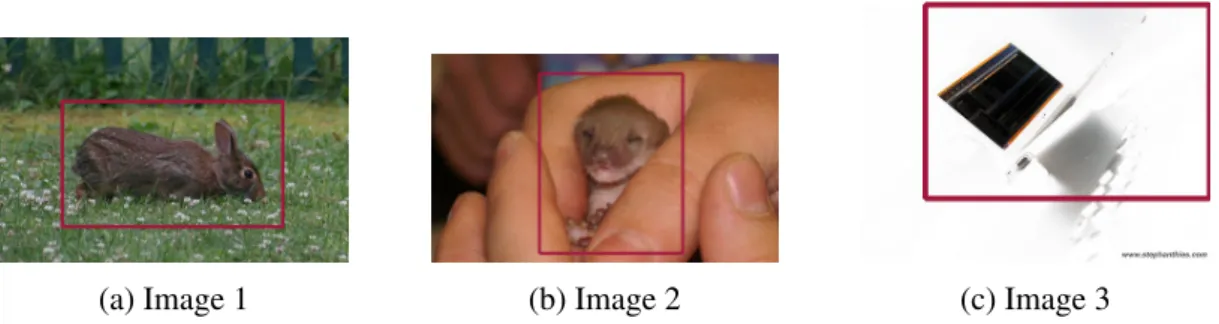
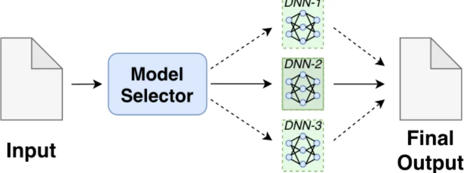
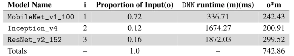
4.1 Motivational Example Images . . . 45

4.2 Inference Time and Optimal DNN of Three Example Images . . . 45

4.3 Example of Ensemble of DNNs . . . 47

4.4 How a Model Selector Would Replace An Ensemble . . . 48

4.5 Thesis Approach Overview . . . 52

4.6 Multi-Classifier Premodel Archtecture . . . 54

4.7 Premodel training process . . . 59

4.8 DNN Specialisation Overview . . . 62

4.9 Data Segmentation Overview . . . 65

4.10 Mean Silhouette Coefficient Across Cluster Feature-Sets . . . 70

4.11 Mean Squared Error Across Cluster Feature-Sets . . . 71

(10)

List of figures x

6.1 Image Classification - Top 5 Feature Importance . . . 88

6.2 Image Classification - Inference Time and Energy Consumption . . . . 89

6.3 Image Classification - Accuracy and F1 Scores . . . 90

6.4 Machine Translation - Feature Importance . . . 94

6.5 Machine Translation - Inference Time, Energy Consumption, and Accuracy 95 6.6 Image Classification - Alternate Premodel Architectures . . . 98

6.7 Machine Translation - Alternate Premodel Architectures . . . 99

6.8 DNN Selection Algorithm Sensitivity Analysis . . . 101

6.9 Image Classification - All Feature Importances . . . 102

6.10 Image Classification - Feature Count Analysis . . . 102

6.11 Machine Translation - All Feature Importances . . . 103

6.12 Machine Translation - Bag of Words Analysis . . . 103

6.13 Premodel Distance Soundness Analysis . . . 106

6.14 Premodel Deep Neural Network Count . . . 107

6.15 Premodel Deep Neural Network Utilisation . . . 108

6.16 Model Selector Approach Resource Utilisation . . . 109

6.17 Compression When Used With Model Selector Performance . . . 110

6.18 Mean Silhouette Coefficient of the Best Performing Feature Sets . . . . 116

6.19 Mean Squared Error of the Best Performing Feature Sets . . . 116

6.20 DNN Specialisation - Comparison of Inference Times . . . 121

6.21 DNN Specialisation - Comparison of Top-1 and Top-5 Scores . . . 122

6.22 DNN Specialisation - Comparison of Precison, Recall, and F1 Scores . 123 6.23 Data Segmentation - Analysis of Segment Sizes . . . 125

6.24 Data Segmentation - Feature Selection Analysis . . . 126

6.25 Data Segmentation - Analysis of Segment Count . . . 127

6.26 Individual Sub-DNN Accurcy Scores . . . 128

6.27 Sub-DNN Creation - Levels of Pruning Analysis . . . 129

6.28 DNN Specialisation Resource Utilisation . . . 130

6.29 Toy Datasets - Comparison of Top-1 and Top-5 Scores . . . 134

(11)

List of tables

3.1 An overview of the work presented in Section 3.1 . . . 27

3.2 An overview of the work presented in Section 3.2 . . . 32

3.3 Research Gap . . . 41

4.1 The Optimal Models for Example Images . . . 46

4.2 Percentage of Important Filters for Example Images . . . 50

4.3 Percentage of Unimportant Filters for Example Images . . . 50

4.4 Model Selector Use Case - Example 1 . . . 54

4.5 Model Selector Use Case - Example 2 . . . 54

4.6 Data Segmentation Example - Candidate Features . . . 68

4.7 Data Segmentation Example - Initial Feature Importance . . . 69

4.8 Data Segmentation Example - Secondary Feature Importance . . . 69

4.9 Data Segmentation Example - Best Feature Sets . . . 69

6.1 Image Classification - Candidate Features . . . 87

6.2 Image Classification - Candidate Feature Correlations . . . 88

6.3 Image Classification - Final Chosen Features . . . 88

6.4 Machine Translation - Candidate Features . . . 93

6.5 Machine Translation - Candidate Feature Correlations . . . 93

6.6 Machine Translation - Final Chosen Features . . . 93

6.7 Model Sizes Changes During Compression . . . 110

6.8 Best Performing Feature Sets After Data Segmentation Search . . . 116

6.9 Features Contained In Each Feature Set . . . 126

6.10 Predictive Power of DNN Specialisation . . . 131

(12)

Nomenclature

Glossary

BLEU A standard machine translation scoring metric.

F1-score A standard machine translation and image classification scoring metric. Calculated from ROUGE and BLEU, or Precision and Recall, for machine translation or image classification, respectively.

Inference The action of a deep neural network making a prediction on an input.

oracle A representation of a perfect machine learning model. That is, a model able to achieve 100% accuracy.

precision A standard image classification scoring metric.

premodel A statistical machine learning model created to make a prediction before a Deep Neural Network is used.

recall A standard image classification scoring metric.

ROUGE A standard machine translation scoring metric.

top-1 A standard image classification scoring metric.

top-5 A standard image classification scoring metric; it is more lenient than top-1.

Acronyms / Abbreviations

CNN Convolutional Neural Network

DL Deep Learning

DNN Deep Neural Network

DT Decison Tree (statistical machine learning model)

GRU Gated Recurrent Unit

K-means K-Means (statistical machine learning model)

KNN K-Nearest Neighbours (statistical machine learning model)

LSTM Long-Short Term Memory

ML Machine Learning

(13)

Nomenclature xiii

NB Naive Bayes (statistical machine learning model)

NMT Neural Machine Translation

NN Neural Network

RL Reinforced Learning

RNN Recurrent Neural Network

SML Statistical Machine Learning

(14)

Chapter 1

Introduction

1.1

Overview

Deep learning is currently one of the key current research areas in machine learning.

Deep Neural Networks (DNN) have proven their ability in solving many difficult and

complex problems, such as: object recognition [24, 43], detecting and recognising objects in an image; facial recognition [102, 123], recognising people from just an image containing their face; speech processing [2, 154], decoding spoken word into text; and machine translation [4, 85, 122], translating text from one language to another. As well as being operated on higher-power servers, many of these deep learning applications are also important application domains for embedded systems [68], especially for sensing and mission critical applications such as health care and video surveillance. Once deep learning technologies become ubiquitous in embedded systems, even greater benefits will be revealed, such as automatous driving, affordable robots for home, augmented reality, and more intelligent personal assistance on mobile phone.

Unfortunately, existing deep learning solutions, which utilise DNNs, are not well

suited to addressing the challenges of embedded systems; they are often resource hungry tasks, demanding a considerable amount of CPU, GPU, memory, and power in order to run effectively [9]. Furthermore, deep learning solutions are becoming more complex in an effort to improve their effectiveness [143]. It is often detrimental, or infeasible, for embedded systems to offer such a large number of system resources to a single task. Without optimization, the hoped-for advances in embedded capabilities will not arrive. The disparity between the resources required and those available will lead to huge energy consumption, reducing battery life, and long inferencing times, making real-time applications infeasible on battery-powered, resource-limited embedded devices.

Numerous optimisation tactics have been proposed to enableDNNinference on

em-bedded devices, hereDNNinference refers to the process of aDNNmaking a prediction

(15)

1.1 Overview 2

drawbacks, such as a reduction in accuracy or an increase in inference time. A common

technique used to accelerateDNNmodels on embedded devices is a process known as

DNNcompression, able to reduce resource and computational requirements of a given

model [32, 35, 36, 50], but this comes at the cost of a loss in precision. To avoid incurring this cost, alternate approaches have been developed; offload some, or all, computation to a cloud server where the resources are available for fast inference times [58, 131]. How-ever, offloading computation into the cloud is often infeasible due to privacy concerns, high latency, or lack of a reliable connection. As such, there is a critical need to find a

way to effectively execute theDNNmodels locally on the devices.

This thesis seeks to offer an alternative approach to executingDNNmodels on

embed-ded systems. The aim is to design ageneralisableapproach toDNNinference optimisation,

making on-device inference feasible without incurring a penalty to model precision, even

when compared to complexDNNssuch asResNet_v2_152. It is not always clear which

DNNis best for the task at hand on embedded devices, therefore the suggested approach

utilises multipleDNNs. Central to the approach is the design of an adaptive scheme

to determine, at runtime, which of the availableDNNs is the best fit for the input and

evaluation criterion. Here, the key insight is that the optimal model – the model which is able to give the correct input in the fastest time – depends on the input data and

the evaluation criterion. In fact, as a by-product, by utilising multipleDNNmodels it

is possible to increase accuracy in some cases. In essence, for a simple input – an image taken under good lighting conditions, with a contrasting background; or a short

sentence with little punctuation – a simple, fastDNNmodel would be sufficient; a more

complex input would require a more complex model. Similarly, if an accurate output

with high confidence is required, a more sophisticated but slowerDNNmodel would need

to be employed – otherwise, a simple model would provide satisfactory results. Given

the diverse and evolving nature of user requirements, applications workloads, andDNN

models themselves, the best model selection strategy is likely to change over time. This ever-evolving nature makes automatic design of statistical machine learning models highly attractive – models can be easily updated to adapt to the changing application context – a user simply needs to supply a set of candidate features.

In order to achieve the goals laid out above, the proposed solution is split into two parts, briefly described below:

Model Selector.By combining classic Statistical Machine Learning (SML) algorithms,

such as K-Nearest Neighbour (KNN), with DNNs, an adaptive scheme is developed to

quickly select the best pre-trainedDNNto use for any given input and the optimization

constraint, at runtime. Anautomaticmethod is proposed, able to dynamically construct

the optimal predictor for eachDNNproblem domain; the user simply needs to supply

(16)

1.2 Motivation 3

automatically tuned features of the DNNinput, the predictor determines the optimum

DNNfor anew, unseeninput; taking into consideration the input and evaluation criterion.

Two typical and uniqueDNNapplication domains are used as case studies for evaluation:

image classification and machine translation. Evaluation is reported on the NVIDIA

Jetson TX2 embedded platform, a wide range of influentialDNNmodels are considered,

ranging from simple to complex. Experimental results show that a Model Selector

approach delivers portable and good performance across the twoDNNtasks. For image

classification, inference accuracy is improved by 7.52% over the most-capable single

DNNmodel while reducing inference time by 44.45%. For machine translation, inference

time is reduced by 25.37% over the most-capable model with negligible impact on the quality of the translation.

DNN Specialisation.Further to a Model Selector, a method of starting with a single seed

DNNand generating a pool of smaller, specialisedDNNsfor the Model Selector to choose

between is proposed; each pool of specialisedDNNsis unique to a problem domain. For

example, consider image classification, each specialisedDNNtailored will be tailored to a

specific subset of the entire range of possible images. Anautomaticmethod is proposed,

able to dynamically separate theDNNtraining data into different segments and train a

number of smallerDNNs. The user simply needs to supply a set of candidate features,

the training data, and a single pre-trainedDNN. Once the newDNNshave been trained

off-linea Model Selector is generated using the above method, able to determine the best

DNNto use, at runtime. Evaluation is reported on the NVIDIA Jetson TX2 embedded

platform, using image classification as a case study. Using this method has the potential to further reduce resource utilisation over using a Model Selector alone, while reducing inference time and increasing inference accuracy by 5.15%. During evaluation, it was not possible to generate an accurate enough Model Selector to reach the full potential of this approach; however, further work (discussed in Section 7.3) points to further areas of investigation to reach this potential.

1.2

Motivation

At the time of writing there are nearly 10 billion mobile and embedded devices currently in use around the world [23] - more devices than there are humans on the planet. Fur-thermore, deep learning technologies are becoming increasingly popular, from image classification to virtual assistants. Many mobile and embedded devices, and their applica-tions, would potentially benefit from the new opportunities enabled by such deep learning

technologies. However,DNNsare inherently computationally and memory intensive. As a

result, it is very challenging to deploy state-of-the-artDNNmodels in resource-constrained

(17)

1.3 Limitations of Current Work 4

As a result, there has been a recent push for more deep learning computation to be executed on device [58, 105]. Some work has investigated off-loading computation, however this is not always an effective solution (discussed further in Section 1.3). The advancement of mobile and embedded systems computational power and architectural diversity has made on-device computation feasible for less expensive - and less accurate

-DNNmodels. Typically, newer devices now contain 8 or more CPU cores of different

levels of energy efficiency, alongside a GPU that can be used forDNNprocessing [124].

Furthermore, mobile operating systems now have in-built support forDNNs; CoreML for

devices running iOS [133], and TensorFlow Lite for Android devices [81]. Furthermore,

recent research has investigated how to build the most effectiveDNNarchitectures for

embedded devices [127]. Such recent advances indicate the demand and popularity for on-device computation. Understandably, it is now common for applications to utilise

DNNs, mobile and embedded devices are a significant source of information and host of

computations in modern technology.

Moreover, there are a number of benefits to on-device computation, including: • Lower Communication Requirements. If all computation is done on device,

there is no need to communicate with a cloud server, therefore less communication bandwidth will be used by the device.

• Less Cloud Computing Costs. It can be expensive for application developers to maintain, or even rent, a cloud server ready to receive requests for deep learning processing. This cost grows as an application becomes more popular too. If deep learning computation is done on device, such costs can be reduced, or even removed entirely.

• Faster Response Times. Further to reducing communication costs, on device computation allows for faster response times. Applications no longer depend on the quality and reliability of cloud servers or mobile network connections, the latter being notorious for unreliability. This benefit is key for mission critical applications such as health care and video surveillance.

• Privacy Preservation. By not communicating with a cloud server, no data needs to leave the device, allowing user privacy to be preserved. Google researchers have

taken this one step further, investigating methods ofDNNtraining on device in an

effort to preserve user privacy [93].

1.3

Limitations of Current Work

Due to the popularity and demand for on-device computation, combined with the huge

(18)

1.3 Limitations of Current Work 5

inference optimisation [21]; typically general purpose optimisation and rarely embedded

devices specific. Relevant research intoDNN optimisation can be summarised into 4

general categories: (i) reducing computational demands, by optimising the underlying

operations in aDNN; (ii) efficientDNNsfor hardware, building more efficientDNN

archi-tectures better suited to mobile archiarchi-tectures; (iii) offloading computation to a server, exploring methods to still offload computation in a smarter way; and (iv) ensemble

learning, utilising more than oneDNNin order to achieve higher accuracy. The benefits

and drawbacks of each of the categories is discussed, in turn, below:

Reducing Computational Demands.There is a wide range of pre-trainedDNNs avail-able. Unfortunately, these networks are often designed to increase accuracy, without much concern for inference times. As a consequence, a number of software-based

approaches have been proposed to accelerateDNNson embedded devices. They aim to

accelerate inference time using methods such as: exploiting parameter tuning [70], com-putational kernel optimization [7, 35], task parallelism [96, 105], and trading precision for time [53]. Work that trades precision for time often yields the greatest optimisation potential, however lower accuracy is undesirable. Since a single model is unlikely to meet all the constraints of accuracy, inference time and energy consumption across inputs [34], it is attractive to have a strategy to dynamically select the appropriate model to use. The work in this thesis presents such a capability and is therefore complementary to these prior approaches.

Efficient DNNs for Hardware. Methods have been proposed to reduce the computa-tional demands of a deep learning model by: trading prediction accuracy for runtime, com-pressing a pre-trained network [12, 37, 106], training small networks directly [32, 107], or a combination of both [50]. Using these approaches, a user now needs to decide when to use a specific model. Making such a crucial decision is a non-trivial task as the application context (e.g. the model input) is often unpredictable and constantly evolving. The work in this thesis alleviates this user burden by automatically selecting an appropriate model to use.

Offloading Computation. Off-loading computation to the cloud can accelerate DNN model inference [58, 131], but this is not always applicable due to privacy, latency or connectivity issues. Recent work attempts to address the issue privacy by obscuring private data before offloading [99], or moving some computation to the device [93, 116, 138]. The work in this thesis aims to advance the effort to perform more computation

on-device, making it a feasible choice when cloud offloading is prohibitive.

Ensemble Learning.By combining multipleDNNstogether, a higher overall accuracy can be achieved. A number of works have investigated how best to do this [104, 144, 86]. The main drawback of such an approach is the huge amount of system resources it

(19)

1.4 Research Questions and Goals 6

requires; mobile and embedded systems often struggle to execute a singleDNN, never

mind multiple in sequence. The work in this thesis is able to utilise the benefits of

ensembles without the drawbacks, by generating DNNs off-line and then adaptively

selecting the bestDNNto use at runtime.

1.4

Research Questions and Goals

It is clear that there is a demand for on-device deep learning inference for mobile and embedded systems. However, despite the efforts of the research community, there is no

clear winner on a single best approach to optimiseDNNsfor embedded inference. This

thesis presents an approach able to combine multipleDNNsinto a single model, allowing

a gain in inference time without a loss in accuracy. Furthermore, work that aims to

improve the efficiency ofDNNmodels can be used in conjunction with the work in this

thesis, applying their techniques to the individualDNNsthat the Model Selector chooses

from. More specifically, this thesis posits the following hypothesis:

By utilising statistical machine learning methods (SML), recent research efforts can be combined to create an adaptive and efficient ensemble-like approach to deep learning inference, without the added costs of conventional ensembles. Furthermore, large deep learning models can be broken down into a set of smaller models capable of achieving the same accuracy for a lower cost.

In order to validate this hypothesis, it is broken down into a set of more specific research questions that will be easier to evaluated. The research questions will be revisited throughout this thesis in order to evaluate the progress of the work. The research questions are formalised below:

[RQ 1] By combining multipleDNNs, is it possible to reduce the average inference time and computational cost across a dataset without causing a reduction in accuracy? Moreover, how much can inference time be reduced by?

[RQ 2] Is it possible to train a statistical machine learning model to choose the optimal

DNN, at runtime, depending on the input and precision requirement?

[RQ 3] Can orthogonalDNNoptimisation techniques such as model compression be used in conjunction with a statistical machine learning model to further reduce inference time without a cost in accuracy?

[RQ 4] Can a set ofDNNsbe generated that are optimised to work together, when combined with a statistical machine learning model, that achieve even further reductions in computational costs and inference times?

(20)

1.5 Research Methodology 7

1.5

Research Methodology

This thesis adopts anexperimentalresearch methodology, using aniterativeapproach

based on aquantitativeanalysis ofprimarydata.

Experimental. In order to investigate the potential effectiveness of a SML model in conjunction with deep learning models, the research questions are broken down into a set of basic experiments, such as those in Section 4.1.1. All experiments are designed

to reveal interesting insights, resulting inprimarydata that is quantitatively analysed in

order to inform future experiments, and update the suggested solutions. Furthermore, experimentation is used to direct the research and further explore areas of an idea that were not originally considered.

Iterative.By adopting an experimental research methodology, new insights are revealed during further experimentation. Therefore, exploration via experimentation is used to inform an iterative approach to repeatedly improve the suggested approaches into more refined and accurate models. An iterative approach works best for this research due to the number of interacting components that all have an impact on one another.

For example, it is not immediately clear what, if any,SMLmodel is able to effectively

utilise multiple DNNs. Therefore, the design of this SML model is initially based on

experimentation choosing the best models based on previous research. Furthermore, once a model is chosen, a decision needs to be made on the best features, and the best

DNNsetc.; The quantitative analysis of the data from, and between, experiments allows

incremental improvements to be made. Intuitively, an iterative approach allows the exploration and analysis of a diverse number of methods in order to achieve the best possible implementation. A detailed experimental evaluation is reported in order to check the feasibility of the final proposed solution.

Quantitative.Finally, a quantitative assessment using real-world data and deep learning models in conjunction with the suggested solutions is used for evaluation. An NVIDIA Jetson TX2 embedded deep learning platform is used for evaluation. It is a single board computer module designed for embedded applications that require high performance

computing [30]. Two popular DNN application domains are considered: image

clas-sification, and machine translation; using the ImageNet ILSVRC 2012 dataset, and

WMT09-WMT14 English-German newstest dataset1, respectively.

Adopting such a research methodology allows for rapid experimentation and analysis during the exploration phase. Furthermore, a quantitative analysis means that the sug-gested approaches can be analysed using techniques used in state-of-the art literature, allowing for clear comparisons.

(21)

Chapter 2

Background

This chapter presents the main concepts of Deep Neural Networks (DNNs) and Statistical

Machine Learning (SML) utilised in this thesis. For clarity, Machine Learning (ML) is

used to mean the broad term that includesSML and DNNs. SMLspecifically refers to

theMLmodels that have a basis in statistics, such as Support Vector Machines (SVMs),

whereasDNNsrefers to theMLmodels based on Neural Networks. This Chapter begins

by introducing different types of learning, as this terminology is common acrossDNNs

andSML. For clarification and conciseness,DNNsandSMLwill be collectively referred to

aslearning modelsin this section. In addition, an in-depth background for bothSMLand

DNNsis presented in their own subsections, before ending with a background in feature

selection and engineering.

2.1

Types of Learning

There are a number of general categories of learning models which are defined by the learning algorithm they use. This Section introduces four of the most prominent learning algorithms: supervised, unsupervised, reinforcement, and online. Below a brief overview of each learning algorithm is given, alongside some examples of common learning models for each. It is worth noting that some learning models can fit into more than one of these categories depending on its use case.

Supervised.In supervised learning the learning model is provided with example inputs that are labelled with their correct outputs. Figure 2.1 presents an overview of the entire supervised learning process, from the original input data to the final predictive model.

Supervised learning begins by distilling the input data into a set oflabelsandfeatures.

Labels are the desired output that the final predictive model should predict when given this input. The features are designed to describe the original input in as few values as

possible,e.g.if the original input is an image, the features could be the average brightness,

(22)

2.1 Types of Learning 9 Label Extractor Feature Extractor Learning Algorithm Training Input Predictive Model labels feature values training data

Fig. 2.1 An overview of the supervised learning process.

values will vary. The combination of features and labels is called thetraining data. The

learning model can then learn from the training data and adjust its internal parameters to

adapt to it throughtraining. If training is successful, the learning model can then predict

the output label fornew, unseeninput data. Supervised learning is commonly used in

optimisation problems, where it is beneficial to predict the best solution to a problem, and the model can be trained off-line [88, 129]. Two categories of supervised learning

that are used in this thesis are: classification, andregression. Classification is based on

discrete output labels,e.g.is there a cat in this picture?; whereas regression is based on

continuous output labels,e.g.given a person’s height, can their weight be predicted?.

Unsupervised.In unsupervised learning the learning model is only supplied with unla-belled input data – only the features. Figure 2.2 shows an overview of the unsupervised learning process; when compared to Figure 2.1 the difference between supervised and unsupervised learning becomes clear. The learning model aims to find commonalities in the input data, and extract some meaningful information, without a reference of a correct output. Often, unlabelled data is much easier to collect than labelled data, making unsupervised learning particularly useful. Commonly, unsupervised learning is used for program optimisation [142, 91], or, commercially in recommender systems. In anomaly detection, the algorithm can draw conclusions about what a "normal" input is, and there-fore indicate when an input fall outside those bounds; this is useful for detecting fraud etc. Recommender systems, such as those used by retailers to suggest new purchases, use unsupervised learning to draw conclusions about past purchases to suggest future

purchases. It is worth noting that there is another kind of learning semi-supervised

learning, where the learning model is provided with some labelled and some unlabelled data. Semi-supervised learning is not used in this thesis.

Reinforcement.Reinforcement learning (RL) is quite different to the learning methods

described so far. InRL, the algorithm is concerned with anagenttaking actions in some

environmentto maximise therewardit will collect alone the way. The idea behindRLis intuitive, if we reward good behaviour and punish bad behaviour, the agent will improve

(23)

2.2 Statistical Machine Learning 10 Feature Extractor Learning Algorithm Training

Input PredictiveModel

feature values

Fig. 2.2 An overview of the unsupervised learning process.

training the algorithm (agent) will learn what is a good or bad move given the current state of the board (environment). Reinforcement learning is not used in this thesis. Online. Online learning is another variation of learning algorithms. In the learning algorithms mentioned above the learning model is supplied with a full training dataset and is tasked with learning its properties to make predictions in the future; the result is astaticpredictor. In online learning the learning model learns as new training data is

produced, and is even able to make predictions during that time; the result is adynamic

predictor. Online learning is useful in environments where it is necessary for the predictor

to dynamically adapt to new patterns in the data, as the patterns arise,e.g.stock price

prediction. Online learning is not used in this thesis.

2.2

Statistical Machine Learning

This section introduces Statistical Machine Learning (SML), a number of commonSML

algorithms that are used in this thesis, and explains some common data preprocessing techniques. For clarification, Machine Learning is a general term that encompasses

DNNsand SML. In this thesis the abbreviationSMLis used to mean Statistical Machine

Learning specifically, whereasMLis used to mean the general term Machine Learning.

SMLapplies the principles of computer science and statistics to create statistical models

which are used for future predictions (based on past data), and identifying patterns in

data. Furthermore,SMLhas been successfully employed for various optimisation tasks,

such as: task scheduling [108], cloud deployment [114], network management [135], etc.

2.2.1

Common Machine Learning Algorithms

This section provides an overview of some commonSMLalgorithms, focussing on the

algorithms that are used in the work within this thesis.

K-Nearest Neighbours.KNNis one of the most popular machine learning algorithms due to its simplicity, leading to quick inference times, and high accuracy on many tasks. In

(24)

2.2 Statistical Machine Learning 11 Feature 2 Feature 1 K=5 Class 2 Class 1 New Point

Fig. 2.3 A 2-class, 2-feature example of the K-Nearest Neighbours algorithm. The point to be classified is represented as a green circle, and its 5 nearest neighbours are enclosed in the dashed ring around it.

Class 2 Class 1

New Point

Fig. 2.4 A 2-class, non-linearly separable example of the Support Vector Machine algorithm. The hyperplane is represented as the dashed line.

Feature 2 Feature 1 Class 2 Class 1 Centroid Data Point (a) Step 1 Feature 2 Feature 1 Class 2 Class 1 Centroid Data Point (b) Step 2 Feature 2 Feature 1 Class 2 Class 1 Centroid Data Point (c) Step 3 Feature 2 Feature 1 Class 2 Class 1 Centroid Data Point (d) Step 4

Fig. 2.5 A 2-cluster, 2-feature example of the K-means Clustering algorithm. (a) The initial random assignment of each data point, (b) Calculate the centroid of each cluster, (c) Re-assign data points to the nearest centroid, (d) Re-calculate centroids of each cluster.

N is the number of input features, and labelling each input point with its output label.

During inferenceKNNtakes the new, unseeninput and finds thek (a hyper-parameter

which is defined by the user) closest training points, which are then used to vote for

the predicted output label. An example of theKNNalgorithm, with k=5, is shown in

Figure 2.3. In this example the five nearest neighbours to the new point (green circle)

are: four red triangles, and one blue square; the final predicted label would beclass 2, as

it is the most frequent label. KNNcan be used for either classification or regression; in

this thesisKNNis used for classification.

K-means Clustering. K-meansis similar toKNN, it is another popular algorithm due

to its simplicity, howeverK-meansis unsupervised. Similar toKNN,K-meansworks by

(25)

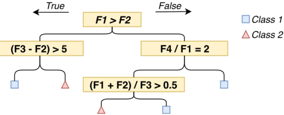
2.2 Statistical Machine Learning 12 F1 > F2 (F3 - F2) > 5 F4 / F1 = 2 True False (F1 + F2) / F3 > 0.5 Class 2 Class 1

Fig. 2.6 An example of a simple decision tree. F1, F2, etc. represent different features, and each box is a different decision in the tree. Each branch of the tree ends in a leaf node representing the class that would be predicted if that branch was followed.

Figure 2.5 shows a simple example of theK-meansalgorithm. To begin, the user sets

the value of k, in this example k=2, which reflects the number of classes the data

should be split into. Each data point is then randomly assigned a class (Figure 2.5a),

and thecentroidof each class is calculated, shown in Figure 2.5b. Data points are then

re-assigned to the nearest centroid; the centroids are then re-calculated. The process of re-assignment and re-calculating is repeated until no more improvements can be made, that is, the mean distance between all centroids and their data points can not be

reduced any more.K-meansresults in each input data point being assigned to one of the

kclusters.

Decision Trees.DTsare simple and computationally cheap, yet effective. An advantage

of DTsis their ability to be easily interpretable and visualised once they are trained;

Figure 2.6 presents and example of a trainedDT. Therootof aDTis the starting point of

all decisions; in the example, the root is the decision ’F1 > F2‘. Every decision is either

true or false, the correspondingbranchis taken depending on the outcome of the decision.

The tree ends inleaf nodes, which are the the class that would be predicted if that leaf is

reached. During training aDTwill try to find the best decisions that split the data most

effectively. The depth and width etc. are controlled using hyper-parameters, however the deeper a tree the more complex it becomes; a balance needs to be struck between

complexity and accuracy of the predictor. Some uses ofDTsinvolve determining the

loop unroll factor [71], and deciding the profitability of GPU acceleration [140].DTscan

be used for either classification or regression problems.

Support Vector Machines. SVMsare another popularSMLalgorithm that are used in

supervised learning, they are more computationally complex thanKNNandDTs, which

allow them to solve more complex problems. During training aSVM will try to draw

a hyperplane between training data points with different labels. In a simple case in

(26)

2.2 Statistical Machine Learning 13

Y

X F(x) -> y

Fig. 2.7 An example of a regression-based curve fitting. Green boxes represent the 6 training examples. The dashed line shows the suggested curve, which maps values

ofxtoy, when plotted on the graph.

R S

0.3

0.4

0.6 0.7

Fig. 2.8 An example of a 2 state Markov Chain. Each state can transition into every other state, including itself; transition are represented as arrows. The probability of each transition labels its arrow.

best separates the data while maximising themargin, that is, the space either side of the

hyperplane that does not contain any data points. Figure 2.4 shows a simple example

of theSVMalgorithm. In this example the new point (green circle) would be classified

as a redclass 2as it is on that side of the hyperplane. Making use ofkernelsin anSVM

increases the computational complexity, but allows the input of non-linearly separable data. A kernel is some functional transformation of the input data, usually to increase the number of dimensions, and allow a linear separation to be found. Once a linear separation has been found the data is mapped back into its original lower-dimensional

space; this is where the curved hyperplane comes from in Figure 2.4. SVMscan be used

for either classification or regression problems.

Logistic Regression.Logistic regression is a widely used supervised learning technique, it is very similar to linear regression, however logistic regression is designed for

non-linear tasks. Contrary toSMLalgorithms such asKNN, regression outputs are continuous,

the approach aims to map values of the input,x, to the output,y, by finding the curve, or

function, f(x). Simply put, logistic regression can be considered ‘curve fitting’. During

training the learning process for logistic regression slightly adjusts the parameters in

f(x)(the current learned curve) to reduce the error between the learned curve and the

data points. Figure 2.7 presents an example of a trained logistic regression model. To begin, the algorithm was presented with six data points which were used to train and

adjust f(x)until the line shown was learned. During deployment ayoutput value can

(27)

useful as a cost estimator, such as predicting execution time [83] or predicting energy consumption [109].

Markov Chain.Markov Chains are a common, and relatively simple, way to statistically model random processes. Conceptually, they model a number of ‘states’, which form a ‘state space’, and the probability of ‘transitioning’ from one state to another. Markov chains are built upon the Markov Property, which states that the transition from one state to another is only dependant on the current state and time, and is independent of the series of states that preceded it [90]. Therefore each transition in a Markov Chain has a probability of likelihood. As every state in a Markov chain can transition into every other state the complexity of the model grows exponentially as more states are added, limiting the number of states a Markov chain can effectively support. Markov chains can be used to generate data based off of a training dataset. As a simple example, a Markov Chain could be used to predict future weather patterns; whether it will be Sunny (S), or Rainy (R). To begin the user would need to supply the model with a list of past data, the Markov Chain will learn the probability of each transition from each state to create the model. Figure 2.8 shows a trained example of the Markov chain with two states: ‘S’, and ‘R’. Markov Chains have been used in previous work for text generation [39] and financial modelling [97].

2.2.2

Statistical Machine Learning Feature Preprocessing

One key aspect in building a successfulSMLmodel is the features. This section introduces

common feature preprocessing techniques that are used in this thesis. Depending on the problem and the domain, a different set of features will be chosen, however there are a set of standard steps a user can take to improve the model’s effectiveness. These steps fall under two main categories: feature scaling and feature selection. Feature scaling is the process of scaling all features to a common range to prevent the range of any single feature being a factor in its importance. Feature selection is the process of reducing our

feature count to improve theSMLmodel’s generalisability. Below, a brief overview of

each of these steps is given.

Correlation.Checking for correlation between features reveals redundant features,i.e.

2 or more features which represent the same information, and drop them, reducing the

computation of theSMLmodel. To calculate the correlation between features, a matrix

of correlation coefficients is constructed. This thesis uses Pearson product-moment correlation (PCC) to produce a matrix, which yields coefficient values between -1 and +1. The closer the absolute value is to 1, the stronger the linear correlation between the two features being tested. A threshold value is then chosen empirically, and any features above the threshold are removed.

(28)

Feature Scaling. The aim of feature scaling is to bring all features into a standard range to improve accuracy; scaling can also bring computational speed-up. Scaling does not affect the distribution or variance of feature values. Scaling can come in a

number of forms, which are effective for differentSMLalgorithms. Standardisation and

normalisation will be covered here. During standardisation feature data is scaled to a mean value of 0, and a standard deviation of 1. To normalise data, it is scaled between the range 0 and 1.

Principal Component Analysis. (PCA) is a linear transformation technique used for feature reduction. PCA aims to reduce the feature count while maximising the feature variance; it is able to remove redundant features. The end goal of PCA is to produce a new feature-set of principal components where there is the minimum correlation (and maximum variance) between the features. Internally, PCA is more complex than simply removing the correlated features. The first principal component is chosen in such a way that it represents the most variability in the original feature-set that is possible. All subsequent principal components are chosen in a similar fashion, however they must also be orthogonal to all preceding principal components. Since the variance between

the features does not depend on theSMLoutput, PCA does not take output labels into

account.

Linear Discriminant Analysis.(LDA), similar to PCA, is an alternate linear transfor-mation technique used for feature reduction. However, LDA relies on output labels to reduce the dimensions of the feature-set. LDA aims to find a decision boundary around each cluster of a class. It then projects the original data points into new dimensions, such that the resulting clusters are as separate from each other as possible; the individual elements of each cluster should be as close to the cluster centroid as possible. Each new dimension is called a linear discriminant. The linear discriminants are ranked based on their ability to: minimise the distance between each centroid and its data points, and maximise the distance between each of the clusters. LDA outperforms PCA in most cases when the input data is uniformly distributed, however LDA requires labelled data. Feature Importance. Often the final step in feature selection is evaluating the impor-tance of each feature, and removing the features which have little impact on the final accuracy. A common way to evaluate feature importance is to first train and evaluate

theSMLmodel using all features, producing a score. In turn, each feature is removed

and theSMLmodel is trained and evaluated again, taking note of the reduction in score.

Intuitively, the features which have little impact on the score when removed are less important, and can be removed. This process can be repeated iteratively to remove a number of features until the accuracy drop is too high.

(29)

2.3 Deep Neural Networks 16

Inputs

Outputs

Input

Layer

Hidden

Layer

Output

Layer

Fig. 2.9 A simple neural network consisting of 3 layers. Blue circles represent individual neurons, which are grouped into layers that are represented by the orange rectangles. Arrows represent connections between neurons.

X₁ X2 X_m

...

W1 W2 W_m

Σ

Output

Inputs

Weights

Weighted

Sum

Activation

Function

Fig. 2.10 The structure of a single neuron of a neural network. This neuron consists ofm

inputs and a single output. Each circle represents data or an operation.

2.3

Deep Neural Networks

SMLmodels are relatively simple and require a user to carefully engineer a set of features.

Deep Neural Networks (DNNs) are capable of solving much more complex problems, and,

in some architectures, can learn the features for the user. This section introducesDNNs,

their terminology, how they work, and some of their applications. In some contextsDNNs

are referred to as Deep Learning (DL), which is seen as a subset of Machine Learning

that refers specifically toDNNs. To begin, this Section gives a brief introduction toDNNs

before moving on to introduce and describe someDNNterminology. Furthermore, this

section describes the specialDNNarchitectures that are specific to this work. Finally,

some relevant applications ofDNNsare described.

2.3.1

Structure

Neural Networks (NNs) are inspired by the human brain, which is made up of neurons,

and connections; connections are formed between neurons. DNNsare a special ‘Deep’

(30)

below) and can be seen as a computer simulation of a brain.DNNsare made up of two

main components:neuronsandconnections. Below, these two components are described

in more detail. They will then be built upon, introducing new components, until a simple

DNN(shown in Figure 2.9) is created.

Neuron.Neurons are a basic unit of aNNthat consist of inputs, an activation function,

and an output. In basicNNs, neuron output is calculated as the weighted sum of the inputs

followed by the neuron’s activation function, which is usually non-linear. This can be

seen in Figure 2.10,minputs (blue) are multiplied by their individual weights (orange),

the sum is taken (green) followed by the neuron’s activation function. The weight of each

input is decided by the input connection. Neurons are organised intolayers. In more

complex and specialisedNNs, neuron output can be calculated differently; explained in

more detail in Section 2.3.3. Unless a neuron is part of theinput layerall of its inputs

are received via connections from other neurons. Finally, unless the neuron is part of the

output layerits output is sent via a connection to one or more neurons.

Connection.Connections are how neurons communicate with each other. Every connec-tion connects one neuron to another, and has a weight. Except between special layers (described in Section 2.3.3), the output of the sending neuron is multiplied by the weight to either increase or decrease the signal given to the receiving neuron. In Figure 2.10 the inputs are the outputs of connected neurons. The weight of a connection will change

duringtraining.

Layer. A layer consists of multiple neurons which are not connected to each other. Layers are connected when the neurons in one layer are connected to the neurons in

another. Figure 2.9 shows a simpleNNconsisting of three layers, an input, output and

hidden layer. Each layer is represented by an orange rectangle; note that the connections are still formed between neurons and not layers. If a layer has no predecessor it is an

input layer, if it has no successor it is an output layer. All layers between the input

and output layers arehidden layers. If the number of hidden layers is large (in general,

more than 8 [66]) then aNN is considered aDNN. ModernDNNscan have hundreds of

layers [149]. There are many different types of specialised layers which are described in more detail later.

2.3.2

Terminology

A usefulDNNis one that can take anew, unseeninput and make an accurate prediction

through a process calledinference. In order to create an accurate DNNit will need to

betrained on some input data (a training dataset in the context of this thesis) using

some set ofhyper-parameters. Below, each of these terms are described in more detail.

(31)

Untrained DNN

DNN Training Algorithm

Dogs Not Dogs Training Dataset

Trained DNN

Fig. 2.11 A simple example of training aDNNto differentiate between images that either

do or do not contain dogs. Each class label in the training dataset (e.g.’dogs’) contains

hundreds or even thousands of images.

Training Datasets. Training an accurateDNNtypically requires a larger amount of data

compared with traditionalNNs. Generally, more and higher quality data results in a better

trainedDNN. In this case data means a set of inputs for theDNNalong with their desired

output, that is, theirclass, orlabel. As a simplified example, to train aDNNto predict

whether an image contains a dog or not then it needs to be provided with twoclassesof

data; Figure 2.11 shows this example. The first is a set of images of dogs, with the label of ‘dog’; and the second is a set of images of anything but dogs, labelled as ‘not dogs’. In real-world applications there are typically hundreds or even thousands of classes

that theDNNwill choose between duringinference. Collecting enough data to train an

accurateDNNthen becomes a huge task. To get around this problem there are a set of

standard datasets for different tasks, each containing huge amounts of data. Two different datasets are used in this thesis: ImageNet ILSVRC 2012 dataset [113] (often referred to as ImageNet), used for image classification; and WMT English-German newstest

dataset1, used for machine translation. It is worth noting that smaller ’toy‘ datasets are

also available, such as MNIST [72] and CIFAR-10 [65]. These datasets consist of fewer classes (around 10, 100x less than ImageNet) and are often used as a proof of concept for

DNNoptimisation tasks, however the results do not always carry over to more complex

problems.

Training.Training aDNNis the process of incrementally updating its weights to reduce

the error of predictions, and increase overall accuracy.Gradient descentis commonly

used to trainDNNs, and is based on an algorithm calledback-propagation; it is an iterative

process ofinference,back-propagation, andweight update. During training theDNNis

given an input, and it produces an output. The inference result could be right or wrong,

which is quantitatively measured by theloss function. Next, the gradient of the loss

function is calculated using back-propagation for each neuron and weight, working from

the output layer backwards. Finally, the weights are updated usinggradient descent.

(32)

Training aDNNoften takes hundreds of thousands of iterations; more training data leads

to more iterations. Training is often measured inepochsinstead of iterations, where each

epoch represents a pass over the entire training dataset.

Inference.The process of aDNNcalculating its output for a given input is called inference,

also known as afeed-forward pass. During inference the input values are given to their

respective input neurons, which calculate their output. The outputs are then passed to the next layer in the network via connections. This process is then repeated for every hidden layer in the network until reaching the output layer, where its output is the output of the network.

Hyper-Parameters. DNNhyper-parameters are settings that can be tuned to influence

the DNN’s behaviour, they are parameters of a DNN that cannot be learned from the

training data. Attempting to learn DNN hyper-parameters directly from the training

data leads to over-fitting, creating a model unable to generalise well to all data. The

number and type of hyper-parameters depend on the type of DNN. Some examples

include: learning rate, which influences the learning progress of aDNN; number of hidden

layers, either increasing or decreasing the model capacity; and convolutional kernel size, deciding the size of a kernel in a convolutional layer (see Section 2.3.3). To guide hyper-parameter tuning during training a validation set of the training data is usually left out. The validation set is then used to test the trained model’s generalisability to new data. Hyper-parameter tuning is usually an expensive and time-consuming process, leading to automatic hyper-parameter tuning libraries being included in frameworks such as TensorFlow.

Pre-Trained Model. Training aDNNrequires a lot of computational power and time. Bigger networks, more training data, and high quality training data typically leads

to a more accurateDNN. Unfortunately, it can also lead to long training times when

specialised hardware is not available. For example, training the simplest version of

ResNet (ResNet_v2_50) on the ImageNet dataset for 90 epochs using an NVIDIA M40

GPU takes 14 days [151]. To makeDNNsmore accessible independent researchers have

trained state of the artDNNarchitectures on complex and freely available datasets such

as ImageNet ILSVRC dataset. They then release the weights of their trainedDNNand

its architecture to the public. A pre-trainedDNN is a combination of the weights and

architecture, which can be downloaded.

Transfer Learning.A pre-trainedDNNcan be used to bootstrap the training of a different

DNNthrough transfer learning. The central concept of transfer learning is to use a more

complex, but successful,DNNto ‘transfer’ its learning to a simpler problem. The key

idea behind transfer learning is that the earlier layers in the DNN have learned some

(33)

Therefore, if the later layer(s) are replaced, they can be retrained for the new problem.

For example, starting with aDNNpre-trained on the ImageNet ILSVRC dataset, transfer

learning can be used to only determine the breed of dog contained in the input image. Transfer learning can take two approaches: simpler fine-tuning, or the more complex representation learning. In fine-tuning only the last couple of layers are replaced and

retrained, to represent the new problem theDNNis solving. These layers are responsible

for producing theDNNoutput values, typically label probabilities. To limit training to

only the new, replaced layers, all other layers would need to befrozen. Representation

learning replaces the last few layers of theDNN with a wholly new model, using the

pre-trained model as a kind of feature extractor. Representation learning is more complex

than fine-tuning as the user is required to design a newNNfor their task, however, it is

more adaptable.

2.3.3

Neural Network Architectures

This section gives an overview of the different types of neural network architectures, and the layers that make each of them unique. The following sections cover: Multi-Layer

Perceptrons (MLPs), and explainfully connected layers; Convolutional Neural Networks

(CNNs), introducingconvolutional, andpooling layers; and Recurrent Neural Networks

(RNNs).

Multi-Layer Perceptrons.

MLPsconsist of at least three layers: an input layer, a hidden layer, and an output layer;

although they can consist of any number of hidden layers. All neurons, except those

in the input layer, use a non-linear activation function. All layers in a MLPare fully

connected in sequence, that is, all neurons inlayer_i are connected to all neurons in

layer_i+1. Figure 2.9 is an example of a small three-layerMLP. Sometimes, MLPsare

referred to as "vanilla" neural networks [42]. MLPsare not directly used in this thesis,

however the architectures that are used build upon them.

Convolutional Neural Networks

For tasks such as image processing,MLPssuffer from several drawbacks, for example

spatial information is lost when flattening the image for input into an MLP. CNNsare

good at capturing spatial information from the input (such as images) through the use of

convolutional layers, which performconvolutions, andpooling layers, which shrink the output and reduce noise within the network. Typically, one or more convolutional layers are followed by a pooling layer. Convolutional and pooling layers are described in more details below.

(34)

Iter 1 Iter 2 Iter 3 Iter 4 Iter 9

...

Fig. 2.12 A red convolutional filter (3x3) is sliding over the blue layer input (5x5). This convolutional layer has a stride of 1, and no padding. The filter slides from left to right, top to bottom.

Iter 1 Iter 2 Iter 3 Iter 4

...

Fig. 2.13 A red convolutional filter (3x3) is sliding over the blue layer input (5x5). This convolutional layer has a stride of 2, and a padding of 1. The filter slides from left to right, top to bottom.

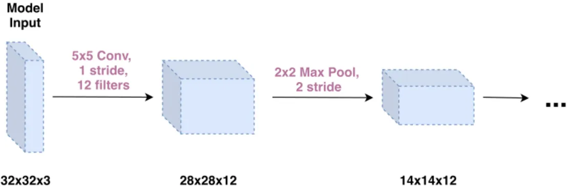
Convolutional Layers.Convolutional layers perform convolutions in place of general

matrix multiplication, which is typically used inMLPs. Each convolutional layer is made

up of a number of filters of a specified size (usually 3x3 or 5x5). The filters are ’moved‘ across the layer input from left to right, top to bottom, performing a matrix multiplication and producing a single output value during each iteration; the layer is convolving the input. Figure 2.12 shows a simple 2D convolutional filter passing over a layer input. As the iteration increases, the filter moves one step right until reaching the edge of the input (iter 3) where it continues on the next row (iter 4). Convolutional layers can also be tuned to have different levels of padding and stride; these values are set per convolutional layer, and are another example of hyper-parameter. Figure 2.13 shows how the convolutional filter interacts with the input when the padding and stride are set to 1 and 2, respectively. For clarification, Figures 2.12 and 2.13 show a single filter of a 2D convolutional layer, this process is repeated for each filter in the layer. In 3D convolutional layers, each filter is the same depth as the layer input, in Figure 2.14 this is 3. During training each

filter will learn to recognise a specific "feature",e.g.eyes, or teeth. Therefore, as each

filter slides across the whole input, aCNNis able to recognise what an image contains,

rather than where an object is. The output of a filter is then passed through an activation function, typically ReLU, which decides if a feature is present at each location in the image, producing a feature map. The output size of a convolutional layer depends on a

(35)

2.3 Deep Neural Networks 22 Model Input 32x32x3 5x5 Conv, 1 stride, 12 ﬁlters 28x28x12 2x2 Max Pool, 2 stride 14x14x12

...

Fig. 2.14 How the data value changes shape as it passes through each layer. Equation 2.1 shows the equation used to calculate output sizes. Data volumes are represented as blue cuboids, and layers are represented as arrows, described in purple text. Input is a 32x32 image with 3 colour channels.

number of factors, and can be formalised in the following equation:

input_size−f ilter_size+2×padding

stride +1 (2.1)

Figure 2.14 shows an example of this equation. Filter outputs are stacked depth-wise meaning the layer output depth is equal to the number of filters. Typically feature maps

are then passed throughpooling layersto shrink the output and reduce noise.

Pooling Layers. Pooling layers are very similar to convolutional layers, they are a special type of convolutional layer used to shrink the output and reduce noise in the network. Pooling works in a similar way to filters, although the pooling operation is specified and not learned, and is typically average pooling, or max pooling. In average pooling, the output value is the average of all the values that the pooling filter can ‘see’, and in max pooling the output value is the maximum. 3D pooling is performed on each ‘depth slice’, meaning the depth is equal before and after a pooling layer. Figure 2.14 shows how the convolutional and pooling layers change the size and shape of data as it passes through the network.

CNNsare usually computation bounded due to the number of matrix multiplications

required in each layer, therefore much research has gone into reducin