Copula-based fuzzy clustering of spatial time series

Copula-based fuzzy clustering of spatial time series

Marta Disegnaa,∗_{, Pierpaolo D’Urso}b_{, Fabrizio Durante}c

a_{Accounting, Finance & Economics Department, Faculty of Management, Bournemouth University, 89}

Holdenhurst Road, Bournemouth, BH8 8EB, United Kingdom

b_{Department of Social Sciences and Economics, Sapienza University of Roma, P.le Aldo Moro 5, 00185}

Roma, Italy

c_{Dipartimento di Scienze dell’Economia, Universit`a del Salento, via Monteroni 165, 73100 Lecce, Italy}

Abstract

This paper contributes to the existing literature on the analysis of spatial time series pre-senting a new clustering algorithm called COFUST, i.e. COpula-based FUzzy clustering algorithm for Spatial Time series. The underlying idea of this algorithm is to perform a fuzzy Partitioning Around Medoids (PAM) clustering using copula-based approach to interpret comovements of time series. This generalisation allows both to extend usual clustering methods for time series based on Pearson’s correlation and to capture the uncer-tainty that arises assigning units to clusters. Furthermore, its flexibility permits to include directly in the algorithm the spatial information. Our approach is presented and discussed using both simulated and real data, highlighting its main advantages.

Keywords: Copula, Fuzzy Clustering, Partitioning Around Medoids, Spatial Statistics, Time Series, Tourism Economics

1. Introduction

Clustering of time series aims to identify similarities in patterns across time. As such, several methods have been developed according to different concepts of similarity that can be based on values, functional shapes, autocorrelation structure, approximation by prototype objects, etc.

Following Caiado et al. (2015) time series clustering methods can be classified into three methodological approaches (for more details, see also Warren Liao, 2005; Caiado et al., 2015; D’Urso et al., 2016a):

1. Observation-based clustering approach: in this case, the methods are based on the observed time series or suitable transformations thereof (see, e.g., Coppi & D’Urso, 2002, 2003, 2006; D’Urso, 2005; Coppi et al., 2010, and references therein).

∗_{Corresponding author}

Email addresses: disegnam@bournemouth.ac.uk(Marta Disegna), pierpaolo.durso@uniroma1.it

2. Feature-based clustering approach: it contains methods that exploit specific features of the time series. For instance, these methods are based on:

• time domain features such as autocorrelation function (ACF) (Alonso & Ma-haraj, 2006; Caiado et al., 2006, 2009; D’Urso & MaMa-haraj, 2009), partial autocor-relation function (PACF) and inverse autocorautocor-relation function (IACF) (Caiado et al., 2006), quantile autocovariance function (QAF) (Lafuente-Rego & Vilar, 2016; Vilar et al., 2017);

• frequency domain features such as periodogram and its transformations (Caiado et al., 2009), coherence (Maharaj & D’Urso, 2010) and cepstral (Maharaj & D’Urso, 2011);

• wavelet features such as wavelet decomposition (D’Urso & Maharaj, 2012; D’Urso et al., 2014);

3. Model-based clustering approach: the methods belonging to this class assume the existence of a stochastic mechanism generating the time series. Moreover, they are based on the fact that a set of time series generated from the same model would most likely have similar patterns. In general, here the time series are clustered by means of the parameter estimates or exploiting the residuals of the fitted models (Caiado et al., 2015). In this class, one can include, among others, methods based on:

• ARMA or ARIMA models (see, e.g., Piccolo, 1990; Maharaj, 1996; Kalpakis et al., 2001; D’Urso et al., 2013b);

• GARCH representation (see, e.g., Caiado & Crato, 2010; Otranto, 2010; D’Urso et al., 2013a, 2016a);

• density function and forecast density (Alonso & Maharaj, 2006; D’Urso et al., 2017).

• functional approach (see, e.g., James & Sugar, 2003);

• splines (see, e.g., Garcia-Escudero & Gordaliza, 1999).

• copulas, measures of association, and tail dependence (see, e.g., De Luca & Zuccolotto, 2011; Durante et al., 2014b; De Luca & Zuccolotto, 2015; Durante et al., 2015; Di Lascio & Giannerini, 2016).

Inside the class of model-based methods, here we focus on the copula-based approach, as recently reviewed in Di Lascio et al. (2017). Copulas are probability distribution functions with uniform marginals, which can be also seen as aggregation functions with special properties (see Durante & Sempi, 2016; Grabisch et al., 2009). They have been extensively used for modelling uncertainty of different types, from probabilistic methods (see Joe, 2015; Nelsen, 2006) to imprecise probabilities and decision theory (see Yager, 2013; Klement et al., 2014; Montes et al., 2015). Nowadays, copula-based models are also frequently used in many problems from spatial statistics; (see, e.g., B´ardossy & Li, 2008; Durante & Salvadori, 2010; Kazianka & Pilz, 2010; Guthke & B´ardossy, 2017).

In stochastic models, copulas are employed in order to represent a joint probability distribution function of a random vector in terms of its marginal distributions. A copula-based model for time series assume that (1) each time series is a realisation of a suitable univariate model (like ARMA, GARCH, ARIMA, etc.) and (2) the innovations (εit) of the individual time series are jointly coupled by means of a time-invariant copula C (see Patton, 2012).

Moreover, since copulas capture the rank-invariant dependence structure of a random vector (see Durante & Sempi, 2016), these algorithms are invariant under strictly increasing transformations of the time series of interest. In other words, two data matrices produce the same cluster composition if one matrix is obtained from the other one by a monotone increasing transformation of its rows (or columns).

Copula-based clustering algorithms for time series are based on this latter decomposi-tion and their specific similarity criterion is derived from the copula informadecomposi-tion (in both parametric and non-parametric form). Such a similarity is often driven by ad-hoc measures of association, like conditional correlations, tail dependence coefficients or variants thereof (see, e.g., De Luca & Zuccolotto, 2011; Durante et al., 2014a,b; De Luca & Zuccolotto, 2015; Durante et al., 2015). Then, in order to identify the partitions, hard clustering algorithms, such as c–means or hierarchical clustering, are usually run on the similarity matrix.

Fuzzy clustering extensions of these methods have been presented in Wang et al. (2017) (for the specific purpose of a portfolio selection algorithm) and in D’Urso et al. (2016b). This latter reference, in particular, suggested the adoption of the copula-based dissimi-larity in the fuzzy Partitioning-Around-Medoids (PAM) algorithm. As known, the main advantage of PAM is that prototypes of each cluster, henceforth “medoid time series”, are time series actually observed and not “virtual” time series, like the “centroids time series” derived by means of thec-means algorithm. The possibility of obtaining non-fictitious rep-resentative time series (i.e. the medoids) is often very appealing for the interpretation of the selected clusters (Kaufman & Rousseeuw, 2005). Moreover, fuzzy clustering algorithms are computationally more efficient (for instance, dramatic changes in the value of cluster membership are less likely to occur in estimation procedures) and they are less affected by both local optima and convergence problems (Everitt et al., 2001; Hwang et al., 2007).

This study aims to revisit the methodology introduced by D’Urso et al. (2016b) for time series, extending these preliminary steps to the problem of classifying spatial units, based on a set of quantitative features observed at several time occasions, namely spatial time series.

One way to cope with the complexity of spatial-time dataset, is to reduce the number of dimensions in order to apply a traditional clustering technique on a two-way matrix. The reduction can be performed in different ways, for example: including the relationships between space and time into a traditional two-way matrix as a new column (Krishnapu-ram & Freg, 1992; Shekhar et al., 2015); adopting the hierarchical time series clustering algorithm where the clustering is performed at different spatial level (Athanasopoulos & Hyndman, 2009). However, this reduction process can cause a loss of information that leads to prefer the development of ad-hoc clustering techniques that incorporate spatial as

well as temporal information. Similar to the classification proposed by Fouedjio (2016) for the clustering of spatial data, existing spatial-time clustering models can be distinguished into the following four different approaches: non-spatial time series clustering based on a spatial dissimilarity measure (Izakian et al., 2013); spatially constrained time series clus-tering (Hu & Sung, 2006; Coppi et al., 2010; Gao & Yu, 2016); density-based clusclus-tering (Ester et al., 1996; Wang et al., 2006; Birant & Kut, 2007; Ienco & Bordogna, 2016; Xie et al., 2016); model-based clustering (Basford & McLachlan, 1985; Viroli, 2011; Torabi, 2014, 2016).

Following this latter approach, a COpula-based FUzzy clustering algorithm for Spatial Time series, shortly COFUST, is proposed and described. In particular, the paper is structured as follows: in Section 2 the suggested algorithm is described and discussed in depth; in Section 3 different simulated case studies are presented in order to show the main features of the algorithm; in Section 4 the methodology is illustrated by analysing real data describing the behaviour of the tourism flows in a destination, i.e. spatial region. Section 5 concludes.

2. The methodology

The starting point is represented by a (n×T)–data matrix,X, defined as follows:

X=        x11 . . . x1t . . . x1T .. . . . . ... . . . ... xi1 . . . xit . . . xiT .. . . . . ... . . . ... xn1 . . . xnt . . . xnT       

where xit is a generic element that represents the value of the i-th unit (i = 1, . . . , n) at the t-th period (t = 1, . . . , T). We also assume to have additional information on units, represented by an (n×n) data matrixS, whose generic entrysij can be interpreted as the “spatial distance” between the i-th andj-th units (i, j = 1, . . . , n). Obviously,sij ≥0.

The clustering process can be split in five consecutive steps: 1. data preprocessing; 2. choice of the appropriate dissimilarity measure; 3. choice of the clustering algorithm; 4. selection of the best partition and cluster validation; 5. profiling and interpretation of the final optimal partition.

The choices made at the first three steps of the clustering process lead to the definition of the proposed COFUST algorithm for time series with spatial information. The first step requires the estimation of a convenient time-series model for each individual time series allowing for the extraction of the corresponding residuals. At the second step of the clustering process, a suitable copula-based dissimilarity measure, that also includes the spatial information between any pair of units xi and xj (i, j = 1, . . . , n and i 6= j), has to be defined. At the third step, the fuzzy PAM algorithm is suggested in view of its valuable advantages. Whereupon, any internal validity measures for fuzzy algorithms suggested in the literature can be adopted both to validate the results and to identify the

best partition that has to be profiled at the final step of the clustering process (Xie & Beni, 1991; Campello & Hruschka, 2006). These steps are presented in figure 1 and described in detail below.

Figure 1: The COFUST steps.

Units Univariate Time Series Spatial information Residuals Time Series Time Series decomposition Empirical Copula Copula Spatial information Eq. (1) Eq. (5) Dissimilarity

measure Fuzzy PAMalgorithm Eq. (6)

Data preprocessing Copula-based dissimilarity Clustering algorithm

2.1. Data preprocessing

In order to disentangle the marginal effects of each univariate time series from the (rank-invariant) dependence properties, it is necessary to conduct a preliminary filtering of the data matrix. Specifically, we can assume that each time series (x1, . . . ,xn) is generated by the stochastic process (Xt,Ft) such that one has

Xit=µi(Zt−1) +σi(Zt−1)εit,

whereZt−1 depends on Ft−1, the available information up to time (t−1), and the innova-tionsεitare distributed accordingly to a probability distribution functionFi. Moreover, the joint distribution function of (ε1t, . . . , εnt) can be expressed in the form of C(F1, . . . , Fn) for some copulaC. Thus,C is not directly related to the original data, but to the residuals obtained after removing from each time series the conditional mean/variance part (see, for instance, Patton, 2012).

Analogously to Durante et al. (2014b, 2015), this pre-filtering serves to mitigates the effects of heteroscedasticity and autocorrelation in the estimation of the dependence struc-ture. In fact, after removing the marginal behaviour, the resulting residuals are approxi-mately a random sample from the copula C.

2.2. Copula-based dissimilarity

The Copula-based dissimilarity measure dij between xi and xj (i, j = 1, . . . , n and

i6=j) can be formalised as a suitable function of the copulaCij (expressing the dependence between the i-th andj-th units) and the spatial information sij.

In the absence of the latter component, a copula-based dissimilarity can be defined as a degree of departure ofCij from the Fr´echet upper-bound copulaM(u, v) = min(u, v), which interprets the maximal degree of similarity (comonotonicity) among time series. Thus, if

Cij =M, the dissimilarity measure betweenxi and xj (i, j = 1, . . . , nandi6=j) is usually set to 0. In D’Urso et al. (2016b), for instance, one sets

dij =f(kM −Cijk),

where k · k is a suitable norm in the copula space, while f is a convenient real-valued function. In order to include also the spatial information in the latter formula, we suggest to proceed as follows.

First, we transform the spatial matrix S, into a matrix whose entries are objects of the copula space. This can be done associating to each pair of units i and j the copula

Sij = ˜sijW + (1−s˜ij)M (1) where W is the Fr´echet lower-bound copula given by W(u, v) = max(u+v −1,0), and ˜

sij =sij/(maxi,j=1,...,nsij) is the normalised spatial distance between thei-th andj-th units. The idea is that, when ˜sij ≈0, i.e. thei-th andj-th units are spatially close, thenSij ≈M, while when ˜sij ≈ 1, i.e. the i-th and j-th units are far away, then Sij ≈ W, which is the copula representing maximal dissimilarity among time series (i.e. countermonotonicity).

Remark 1. Notice that (1) defines an element of the Fr´echet family of copulas (see, for instance, Durante & Sempi, 2016). Clearly, other parametric families of copulas can be chosen as well, provided that they are comprehensive (i.e. they include W and M as elements) and ordered (with respect to concordance as defined, e.g., in Durante & Sempi, 2016).

Second, we associate to each pair (i, j) of units a copula that merges dependence and spatial information, namely

e

Cij =βCij + (1−β)Sij, (2) whereβ ∈[0,1] is a tuning parameter (we recall that any convex combination of copulas is a copula). Roughly speaking,Ce_ij combines both the dependence and the spatial information

among the units i and j. The parameter β ∈ [0,1] reflects the prior belief of the decision maker about the desired influence of the spatial component on the clustering procedure. If the aim is to obtain a clustering output that only reflects the dependence information between units, theβparameter has to be set equal to 1. As much as the spatial information is considered to be relevant for the clustering analysis,β has to take smaller values.

Finally, we define the dissimilarity measure as

dij =f(kM −Ceijk), (3) where k · k is a suitable norm in the copula space (like the Cr´amer-von Mises L2_–norm,

k · k2, and the Kolmogorov-Smirnov norm or L∞–norm, k · k∞), while f is an increasing

and continuous real-valued function with f(0) = 0. Notice that, regardless the value of

dependence between the units is very strong, i.e. Cij ≈M. In other words, if the units are spatially adjacent and their time series are comonotone, then their dissimilarity is equal to 0, while the dissimilarity increases when we have a small deviation from such limiting case.

Remark 2. Eq. (3) can be rewritten as

dij = f(kM −βCij −(1−β)Sijk

= f(kβ(M −Cij) + ˜sij(1−β)(M −W)k), (4) which emphasizes the role played by both spatial and dependence information in the de-termination of the dissimilarity measure.

Remark 3. Given any two time series (xit)t=1,...,T and (xjt)t=1,...,T related to thei–th and

j–th units, the copulaCij (and, hence, the related dissimilarity computed following eq. (3)) can be estimated either parametrically or non-parametrically. In the latter case, we can use the empirical copula

Cij(u, v) = 1 T T X t=1 1 Rit T + 1 ≤u, Rjt T + 1 ≤v , (5)

where Rit and Rjt are the ranks associated with the (residuals of) original time series.

2.3. Clustering algorithm

The COFUST clustering algorithm can be formalised as follows:

min uik : n X i=1 K X k=1 up_ikdik(xi,xk) = n X i=1 K X k=1 up_ikf(kβ(M −Cik) + ˜sik(1−β)(M −W)k) s.t. K X k=1 uik = 1, uik ≥0 (6)

where uik indicates the membership degree of the i-th unit in the k-th (k = 1, . . . , K) cluster;p > 1 is a weighting exponent that controls the fuzziness of the obtained partition;

xk represents the time series of the medoid of the k-th cluster; dik(xi,xk) is the copula-based dissimilarity measure (see subsection 2.2) computed between the time series of the

i-th unit and the time series of the k-th medoid.

Remark 4. Notice that the fuzziness parameter p is chosen in advance and plays an important role in fuzzy clustering and, in particular, in our fuzzy PAM clustering method. In fact, if p is close to 1, the algorithm output will result in a partition with most of the memberships close to 0 or 1. Conversely, choosing a large p will lead to disproportionate overlap with all memberships close to 1/K (see, e.g., Wedel & Steenkamp, 1989). For

this reason, Kamdar & Joshi (2000) recommended to select a value of p included in the range (1,1.5]. Although there have been some empirical heuristic procedures to determine the value of p, there seems to exist no theoretically justifiable manner of selection. For a discussion and a detailed list of references on the choice of p, see also D’Urso (2015).

Remark 5. In general, internal validity measures provide useful guidelines in the identi-fication of the best partition (as suggested by Handl et al., 2005; D’Urso, 2015). Suitable measures for fuzzy clustering algorithm have been suggested by Xie & Beni (1991) and Campello & Hruschka (2006). Among them, the Fuzzy Silhouette (F S) index (Campello & Hruschka, 2006) is a popular measure that is computed as the weighted average of the individual silhouettes width, λi, as follows:

F S= Pn i=1(uir−uiq)α·λi Pn i=1(uir−uiq)α , λi = (bi−ai) max{bi, ai} (7) Here, ai is the average distance between the i-th unit and the units belonging to the cluster r (r = 1,...,k) with which i is associated with the highest membership degree; bi is the minimum (over clusters) average distance of the i-th unit to all units belonging to the cluster q with q 6= r; (uir −uiq)α is the weight of each λi calculated upon the fuzzy partition matrix U = {uik;i = 1, . . . , n, k = 1, . . . , K}, where r and q are, respectively, the first and second best clusters (accordingly to the membership degree) to which thei-th unit is associated; α ≥ 0 is an optional user defined weighting coefficient. Note that, the traditional (crisp) Silhouette measure is obtained by setting α = 0. The higher the value of F S, the better the assignment of the units to the clusters simultaneously obtaining the minimisation of the intra-cluster distance and the maximisation of the inter-cluster distance.

Remark 6. Regarding the comparison between two partitions, different measure of par-tition correspondence have been suggested in the literature based on the well-known Rand index (Rand, 1971). Here we adopt the Adjusted Rand Index (ARI) computed as:

ARI = n 2 2a−2(a+b)(a+c) n 2 [(a+b) + (a+c)]−2(a+b)(a+c) (8) whereais the number of pairs objects placed in the same group in both partitions, b andc

count the number of time two objects are paired only in one partition, and n₂is the total number of possible combinations of pairs. The ARI index assumes value 1 when perfect match between the two partitions is found (for more details see Hubert & Arabie, 1985).

In the fuzzy framework, one of the most recent and frequently used measure is the Fuzzy Rand Index (FRI) suggested by H¨ullermeier et al. (2012) and defined as follows:

FRI = 1− P (xi,xj)∈K|E A_(x i, xj)−EB(xi, xj)| n 2 (9)

where A and B are two fuzzy partition, EA_(x

i, xj) = 1− kuAi −uAjk, k · k is any norm on [0,1]K_{, u}A

unit in thek-th cluster of theAfuzzy partition. Therefore, the FRI takes values between 0 and 1. The closer the FRI value to 1 the higher the similarity between two fuzzy partition.

3. Illustration with simulated data

Here we illustrate the COFUST algorithm under various simulation setups, showing its main performance and features. In this section, we assume that the dissimilarity measure of eq. (3) is computed via the empirical copula, the norm k · k is the L2 _{or the L}∞ _norm

(which are commonly used in various goodness of fit tests for copulas as copula distances, see Genest et al., 2009), the function f is set equal to f(t) = exp(t)− 1. This latter choice has been empirically tested and seems to be the most convenient to highlight small differences among dissimilarity values, but clearly other functionsf could be used provided that f is increasing with f(0) = 0. Finally, the fuzzy parameterp in eq. (6) is set equal to 1.5. This is the maximum value suggested by Kamdar & Joshi (2000) and for values of p

lower than 1.5, but higher than 1, the final partition becomes less fuzzy.

The other parameters to be set are: the tuning parameter β ∈[0,1], the spatial matrix

S, the final number of clusters K, the copula model describing the dependence among the

n innovations of lengthT. For simplicity, we assume that the number of clusters is always well identified, while the cluster composition is clearly unknown. Below, several cases are considered and described.

3.1. Case 1: clustering of time series without spatial information

First, we check the ability of the methodology to identify correctly the cluster compo-sition when no spatial information is included (i.e. β = 1).

We considern= 100 time series of innovations of lengthT ∈ {100,200}. For simplicity, we assume that the time series are grouped in k = 2 clusters and, specifically, they are generated via the following copula model:

C(u1, . . . , u100) =C1(u1, . . . , u50)·C2(u51, . . . , u100), (10) whereC1 andC2 are copulas belonging to the families of Frank, Clayton, and Gumbel with a pairwise Kendall’sτ in{0.1,0.25}. As known, these families describe three different situ-ations in terms of tail properties, namely asymptotic independence in the lower and upper tail (Frank), asymptotic dependence in the lower tail (Clayton), asymptotic dependence in the upper tail (Gumbel). In other words, the time series are divided into two clusters that are independent each other, while the dependence within clusters is given by the copulas

C1 and C2 respectively.

For each replication R = 1, . . . ,250, we simulate from model (10) and we apply CO-FUST algorithm to determine the membership degree of each time series belonging to the two clusters. In order to evaluate whether the time series are adequately classified or not, we compute the percentage of correctly classified time series and the percentage of non-fuzzy assignments. To obtain the last percentage, we consider a non-non-fuzzy a time series associated to a cluster with a membership degrees higher or equal to 0.7, as suggested by

Family Correct (%) Non-Fuzzy (%) ARI FRI Clayton (τ = 0.10) 86.8080 54.0600 0.5675 0.6149 Clayton (τ = 0.25) 99.6960 95.5400 0.9880 0.8401 Gumbel (τ = 0.10) 79.6320 44.3160 0.4007 0.5785 Gumbel (τ = 0.25) 99.6720 94.9160 0.9870 0.8350 Frank (τ = 0.10) 86.5400 53.0840 0.5549 0.6129 Frank (τ = 0.25) 99.8200 96.7760 0.9928 0.8550

Table 1: Results of COFUST algorithm (based on L2 norm) ) with dissimilarity measure obtained from (4) (β = 1) related to simulated data of length T = 100 from model (10). Mean values over R = 250 replications.

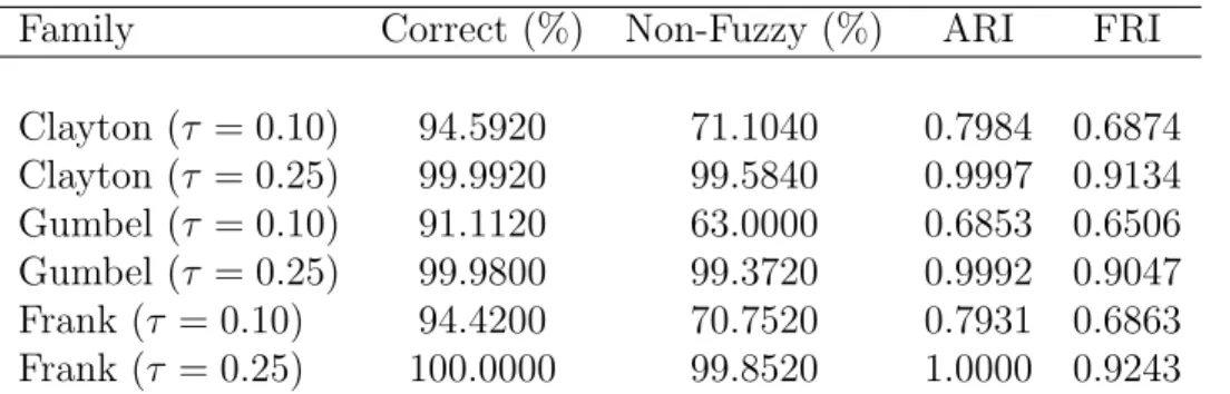
Family Correct (%) Non-Fuzzy (%) ARI FRI

Clayton (τ = 0.10) 94.5920 71.1040 0.7984 0.6874 Clayton (τ = 0.25) 99.9920 99.5840 0.9997 0.9134 Gumbel (τ = 0.10) 91.1120 63.0000 0.6853 0.6506 Gumbel (τ = 0.25) 99.9800 99.3720 0.9992 0.9047 Frank (τ = 0.10) 94.4200 70.7520 0.7931 0.6863 Frank (τ = 0.25) 100.0000 99.8520 1.0000 0.9243

Table 2: Results of COFUST algorithm (based on L2 _{norm) ) with dissimilarity measure obtained from}

(4) (β = 1) related to simulated data of length T = 200 from model (10). Mean values over R = 250 replications.

D’Urso et al. (2017). Moreover, we calculate the ARI (eq. 8) and the FRI (eq. 9) to quantify how much the obtained group composition matches with the theoretical one.

The results obtained using the L2 _{norm are reported in Table 1 (for the case T = 100)} and Table 2 (for the case T = 200). Analogously, the results obtained using theL∞ norm are reported in Table 3 (for the caseT = 100) and in Table 4 (for the case T = 200).

The results can be summarised as follows:

• At the increase of the length T of the time series, the overall performance improves (as expected).

• Regardless the chosen copula family, if we increase the dependence parameter τ, the algorithm performs better, identifying more separated clusters. However, it seems to perform slightly worse when the data are generated from Gumbel copulas.

• Given all the other parameters fixed, the dissimilarity based onL2 norm seems to be more capable than theL∞norm in the identification of the true cluster composition. In order to check whether the previous performance may depend on the number of

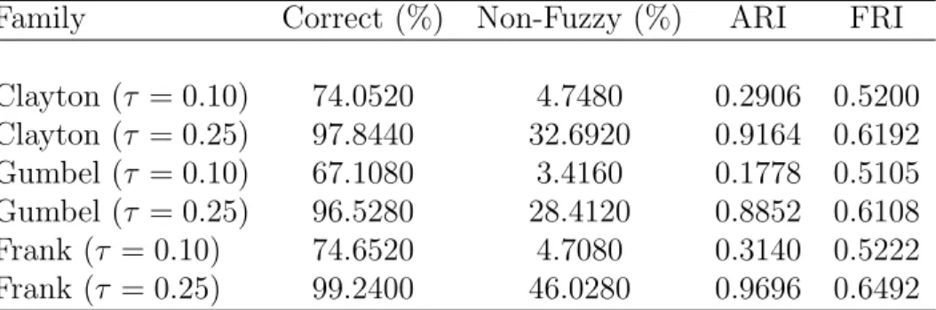
Family Correct (%) Non-Fuzzy (%) ARI FRI Clayton (τ = 0.10) 74.0520 4.7480 0.2906 0.5200 Clayton (τ = 0.25) 97.8440 32.6920 0.9164 0.6192 Gumbel (τ = 0.10) 67.1080 3.4160 0.1778 0.5105 Gumbel (τ = 0.25) 96.5280 28.4120 0.8852 0.6108 Frank (τ = 0.10) 74.6520 4.7080 0.3140 0.5222 Frank (τ = 0.25) 99.2400 46.0280 0.9696 0.6492

Table 3: Results of COFUST algorithm (based on L∞ norm) ) with dissimilarity measure obtained from (4) (β = 1) related to simulated data of length T = 100 from model (10). Mean values over R = 250 replications.

Family Correct (%) Non-Fuzzy (%) ARI FRI

Clayton (τ = 0.10) 84.2280 2.1920 0.5063 0.5263 Clayton (τ = 0.25) 99.7800 21.3440 0.9912 0.6252 Gumbel (τ = 0.10) 75.1000 1.9400 0.3467 0.5165 Gumbel (τ = 0.25) 99.7400 21.6240 0.9897 0.6265 Frank (τ = 0.10) 85.9000 2.3600 0.5795 0.5338 Frank (τ = 0.25) 99.9440 37.4720 0.9978 0.6529

Table 4: Results of COFUST algorithm (based on L∞ norm) ) with dissimilarity measure obtained from (4) (β = 1) related to simulated data of length T = 200 from model (10). Mean values over R = 250 replications.

Family ARI FRI ARI FRI T = 100 T = 100 T = 200 T = 200 Clayton (τ = 0.10) 0.3153 0.4652 0.5763 0.5290 Clayton (τ = 0.25) 0.9791 0.7333 0.9994 0.8404 Gumbel (τ = 0.10) 0.2310 0.4467 0.4541 0.5009 Gumbel (τ = 0.25) 0.9641 0.7170 0.9985 0.8257 Frank (τ = 0.10) 0.3051 0.4624 0.5868 0.5334 Frank (τ = 0.25) 0.9866 0.7521 0.9999 0.8556

Table 5: Results of COFUST algorithm (based onL2_{norm) with dissimilarity measure obtained from (4)}

(β = 1) related to simulated data of lengthT ∈ {100,200} from model (11). Mean values over R= 250 replications.

clusters, we also consider the following 128–dimensional copula model:

C(u1, . . . , u128) = 4

Y

i=1

Ci(u1+32(i−1), . . . , u32+32(i−1)), (11)

where Ci is a copula belonging to the families of Frank, Clayton, and Gumbel with a pairwise Kendall’s τ in {0.1,0.25}. In other words, the model considers four independent clusters, each of them composed by 32 time series. The results are summarised in Table 5. As can be noticed, the performance of COFUST seems to be independent from the number of clusters.

3.2. Case 2: clustering of time series with spatial information

Given the previous simulation setup, one may wonder whether the presence of spatial information may increase the membership degree of some units to a specific cluster. To this end, we consider n= 100 time series of innovations of lengthT = 100. The time series are generated through the copula models specified in (10), where C1 and C2 are copulas belonging to the families of Frank, Clayton, and Gumbel with a pairwise Kendall’sτ = 0.1. The spatial matrix is defined in such a way that sij = 0 when either i, j ∈ {1, . . . ,50} or

i, j ∈ {51, . . . ,100}, otherwise sij = 1. In other words, two units linked by eitherC1 orC2 are also spatially close to each other.

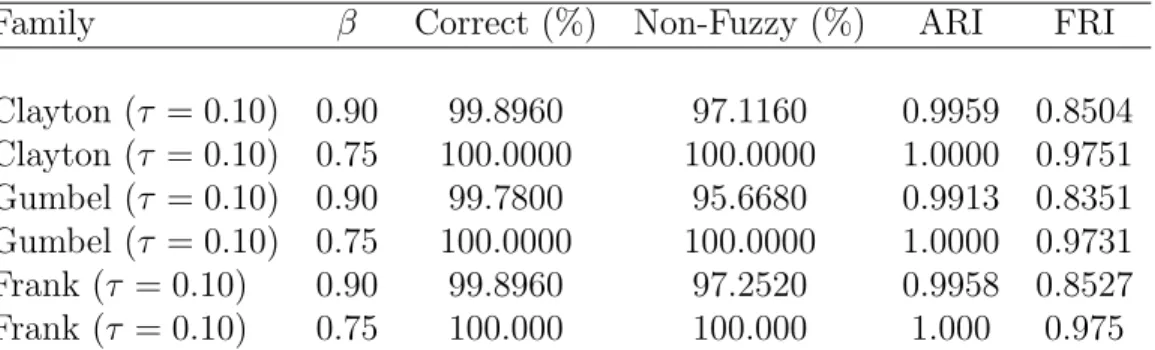
As before, for each replication, we compute the percentage of correct classifications, whether the assignment is fuzzy or non-fuzzy, and we calculate the ARI and FRI indices. The results are reported in Table 6. As can be seen, the spatial information seems to influence the cluster composition even for values of β sufficiently close to 1 (that is the limiting case when no spatial information are considered).

Therefore, it seems critical for the correct application of the algorithm to determine a value ofβ that is consistent with the decision maker’s attitude towards a group composition that reflects the spatial grouping of the time series. To this end, we run a final experiment and we consider n = 50 time series of length T = 100. We assume that the time series

Family β Correct (%) Non-Fuzzy (%) ARI FRI Clayton (τ = 0.10) 0.90 99.8960 97.1160 0.9959 0.8504 Clayton (τ = 0.10) 0.75 100.0000 100.0000 1.0000 0.9751 Gumbel (τ = 0.10) 0.90 99.7800 95.6680 0.9913 0.8351 Gumbel (τ = 0.10) 0.75 100.0000 100.0000 1.0000 0.9731 Frank (τ = 0.10) 0.90 99.8960 97.2520 0.9958 0.8527 Frank (τ = 0.10) 0.75 100.000 100.000 1.000 0.975

Table 6: Results of COFUST algorithm (based onL2norm) with dissimilarity measure obtained from (4) (β∈ {0.75,0.90}) related to simulated data of lengthT = 100 from model (10). Mean values overR= 250 replications.

are grouped in k= 2 clusters and that the first two time series are linked by a copula C1, while the other time series are linked by a copula C2. Moreover, we assume that the first two units are independent of the remaining ones. Since the choice of the copula family does not play a major role in the performance of COFUST, the copula model is set to be

C(u1, . . . , u50) = C1(u1, u2)·C2(u3, . . . , u50), (12) whereC1 andC2 are Frank copulas with a pairwise Kendall’sτ in{0.5,0.75}. The spatial matrix is defined in such a way that sij = 0 when both i, j ∈ {2, . . . ,50}, while s1j = 1 for every j 6= 1. In other words, the first time series is maximally far from the other time series that, conversely, are spatially close to each others.

Figure 2 reports the membership degree of unit 2 to the same cluster of unit 1 at different levels of β. Clearly, when β = 1 (i.e. no spatial information) units 1 and 2 tend to belong to the same cluster, since they are dependent via the copulaC2. However, when

β decreases, the spatial component plays a major role and, roughly speaking, it moves unit 2 far from unit 1, i.e. in a different cluster. Finally, it is important to highlight that, regardless the value of the dependence parameter τ, the membership degree of unit 2 to the same cluster of unit 1 is very high for values of β included in the interval [0.6,0.9], while for β lower than 0.5 it becomes approximately 0.

4. A case study with economic data

A tourism agglomeration can be defined as a geographic concentration of interconnected tourism businesses that cooperate (but also compete) creating a network of relationships that allows them to perform better certain tourism economic activities (see, e.g., Yang, 2012). As such, the detection of the existence of agglomeration of touristic sites and the analysis of their trend over time-space is recognised as a key factor in promoting tourism development (Yang, 2012).

Here we exploit the COFUST algorithm in the problem of finding a common behaviour of touristic flows. Specifically, given a geographic region having various localities as pos-sible touristic attractions, we aim at identifying agglomerations of cities characterised by

0.2 0.4 0.6 0.8 1.0 0.0 0.2 0.4 0.6 beta Membership degree 0.2 0.4 0.6 0.8 1.0 0.0 0.2 0.4 0.6 0.8 1.0 beta Membership degree

Figure 2: Results of COFUST algorithm (based on L2 _{norm) with dissimilarity measure obtained from}

(4) (β ∈[0,1]) related to simulated data of lengthT= 100 from model (12) with Kendall’sτequal to 0.50 (left) and 0.75 (right). Mean values over R= 50 replications.

a common trend of the tourist flows over time and, eventually, by a geographic close-ness. Adopting the suggested COFUST algorithm, we have the opportunity to: 1) identify agglomerations of cities made up considering both common tourist flow trends and geo-graphical proximity; 2) recognise the medoid of each agglomeration, i.e. the municipality that characterises each agglomeration and that can be considered as the representative touristic municipality (in statistical terms) of a given sub-region.

In this analysis, we consider monthly tourist arrivals in the municipalities located in South-Tyrol region (Northern Italy) collected by ASTAT (the local institute of statistics) from 2008 to 2014. South–Tyrol is a tourist destination characterised by 116 municipalities grouped into eight administrative districts that follow the geomorphology of the region.

The distance (in meters) between each pair of towns/villages has been calculated by ISTAT (the national institute of statistics) using a commercial street map (TomTom’s MultiNet). The normalised spatial distance between pair of units has been used in the calculation of the copula-based dissimilarity as described in sections 2.2.

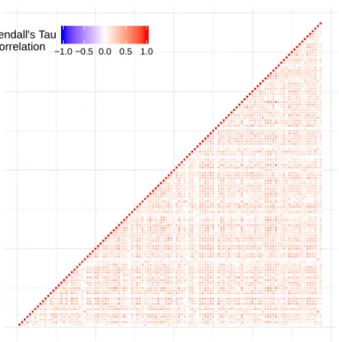
Individual time series show the presence of a seasonal component, which should be removed before calculating the dissimilarity measure (as described in sections 2.1). To this end, each time series has been separately fitted via a seasonal ARIMA model whose order has been selected accordingly to the stepwise procedure suggested by Hyndman & Khandakar (2008) (output of the analysis available upon request). The resulting residuals from the time series are hence used to determine the copula-based dissimilarity. First of all, we should notice that the pairwise dependence among the residual time series is low, as can be observed from the pairwise Kendall’s measure of association represented in Figure 3.

Figure 3: Heatmap of the pairwise Kendall’s correlation between residuals time series. 0 30 60 90 120 0 30 60 90 120 −1.0 −0.5 0.0 0.5 1.0 Kendall's Tau Correlation

In order to provide an estimation of the copula among each pair of time series, we consider hence the empirical copula as in eq (5). Then, the dissimilarity measure has been calculated by means of eq. (3) where the L2–norm has been selected and the function f

has been set equal to f(t) = exp(t)−1 (as in the simulation study). Finally, the obtained dissimilarity matrix has been used as input of the optimisation problem (6) settingp= 1.5. The algorithm has been performed under different levels of both spatial information (i.e. different choices ofβ) and number of clusters k. Figure 4 summarises the values of the FS Index calculated for kfrom 2 to 10 and forβ from 1 (no spatial information) to 0.5 setting

α= 1 (as suggested by Campello & Hruschka, 2006). The choice of theβ−values has been made accordingly to the simulation results that revealed that for β−values lower than 0.5 the effect of spatial information is too high. The trajectories showing the FS values suggest that, regardless β, the best partition isk = 2.

For an easy comprehension of the final results, the membership degrees of each town/village, along with the medoids of each cluster, are represented in figure 5 where: map 6(a) shows the results obtained considering only the empirical copula (i.e. the dependence among time series); while map 6(f) shows the results obtained weighing equally the empirical and spatial copulas, i.e. β = 0.5.

As expected, the higher the weight of the spatial information, the higher the proportion of non-fuzzy units and higher the spatial separation between the clusters. However, for this case study, an optimal value of β seems to be β = 0.7 since the medoids are quite stable and the level of spatial separation between the clusters is satisfactory. Focusing on this

● ● ● ● ● ● ● ● ● Number of clusters FS ● ● ● ● ● ● ● ● ● 2 3 4 5 6 7 8 9 10 0.10 0.20 0.30 0.40 0.50 0.60 ● ● β =1 β =0.9 β =0.8 β =0.7 β =0.6 β =0.5

Figure 4: COFUST Algorithm applied to touristic flows time series (see text). Values of the Fuzzy Silhouette Index for each cluster partition forkfrom 2 to 10, varying β from 1 to 0.5.

final cluster solution (figure 6(d)), we can notice that the two medoids are geographically far, they belong to two separate and not adjacent valleys. In particular, Tesimo belongs to the Adige valley, well-known for summer holidays, while Bressanone belongs to the Isarco valley, one of the biggest valleys in South-Tyrol mainly characterised by winter attractions. From a managerial point of view, a two-clusters partition sometimes cannot be fully informative and the analysis of the second-best partition is often recommended (D’Urso et al., 2015). From the inspection of the F S index curve (see figure 4), the second-best partition obtained setting β = 0.7 is k = 7. The membership degree of each town/village, along with the medoid of each cluster, are represented in maps 7(a)-7(g) for an easy interpretation of the results. In map 7(h), the final medoids are compared with the districts to whom they belong from an administrative point of view. As we can observe, Campo Tures and San Lorenzo di Sebato belong to the same administrative district, but they are the medoids of two different clusters. The same situation can be observed for Lagundo and Gargazzone in the Burgraviato. Conversely, Bressanone seems adequate to represent not only Valle Isarco, the district to which it belongs, but also the Alta Valle Isarco. The Salto-Scilliar district is represented by a combination of two medoids, Bressano and Montagna. Finally, Bolzano, the biggest municipality of South-Tyrol, is mostly associated to the cluster represented by Gargazzone with which it shares similar co-movements in the tourism flows.

Summarising, we can argue that, tourist flows policies created on the basis of the existing administrative districts are not always well representative of the real situation of the region. Their use is hence subject to caution and should take into consideration also the co-movement of tourists in the different localities in order to further enhance the promotion of ad-hoc managerial and marketing policies for regional tourism development.

Figure 5: Distribution of the membership degrees for the best partition obtained varyingβ from 1 to 0.5. The city-medoids of the best partitions are highlighted in each map.

(a) (b)

(c) (d)

Figure 6: Distribution of the membership degree for the second-best partition obtained setting β = 0.7 (maps 7(a)-7(g)) and districts distribution (map 7(h)). The city-medoids are highlighted in each map.

(a) (b)

(c) (d)

(e) (f)

5. Conclusions

In this paper a new clustering algorithm for spatial-time series, i.e. the COpula-based FUzzy clustering algorithm for Spatial Time series (COFUST), has been presented. In particular, the aim is to identify cluster of time series in which the dependence is identify through a copula-based approach and the spatial information regarding units are included in the clustering algorithm. The PAM clustering algorithm has been adopted in order to identify actual units, i.e. time series, representing the final clusters since the possibility to interpret the results using non-fictitious units is appealing in many real applications. Moreover, the fuzzy approach has been adopted since it is well known that fuzzy clustering algorithms are computationally more efficient, they tend to be less affected by both local optima and convergence problems. Furthermore, the possibility to belong to more than one cluster simultaneously allows to cope with the uncertainty in the unit assignments.

Different simulation studies and a real case study have been presented to illustrate the usefulness and effectiveness of the suggested clustering method for spatial-time series. In particular, the findings of the simulation studies suggest that, in the absence of spatial information and regardless the copula family selected, the COFUST tends to identify the true cluster composition. Moreover, the inclusion of spatial information in the clustering algorithm affects the cluster composition, pushing units weakly dependent, but spatially close each other, in the same cluster. Here, the value for the tuning spatial parameter β, that defines the weight of the spatial information in the calculation of the dissimilarity between each pair of units, plays a crucial role.

The application to the real case study shows that the COFUST algorithm may help in the selection of groups that are both dependent and spatially close, making more appealing the applicability of the results of the cluster analysis.

Acknowledgment

The third author was partially supported the Free University of Bozen-Bolzano, Faculty of Economics and Management, via the project AIDA. Moreover, he also acknowledges the support of Cost Action CRoNoS - IC1408, supported by the EU Framework Programme Horizon 2020.

References

Alonso, A., & Maharaj, E. (2006). Comparison of time series using subsampling. Comput. Stat. Data Anal.,50, 2589–2599.

Athanasopoulos, R., G. Ahmed, & Hyndman, R. (2009). Hierarchical forecasts for Australian domestic tourism. Int, J. of Forecast.,25, 146–166.

Basford, K., & McLachlan, G. (1985). The mixture method of clustering applied to three-way data. J. Classification, 2, 109–125.

Birant, D., & Kut, A. (2007). ST-DBSCAN: An algorithm for clustering spatial-temporal data. Data Knowl Eng.,60, 208–221.

Caiado, J., & Crato, N. (2010). Identifying common dynamic features in stock returns. Quant. Finance,

10, 797–807.

Caiado, J., Crato, N., & Pe˜na, D. (2009). Comparison of times series with unequal length in the frequency domain. Comm. Statist. Simulation Comput.,38, 527–540.

Caiado, J., Crato, N., & Pe˜na, D. (2006). A periodogram-based metric for time series classification.

Comput. Stat. Data Anal.,50, 2668–2684.

Caiado, J., Maharaj, E. A., & D’Urso, P. (2015). Time series clustering. In C. Hennig, M. Meila, F. Murtagh, & R. Rocci (Eds.),Handbook of Cluster Analysis (pp. 241–264). Chapman and Hall/CRC.

Campello, R. J., & Hruschka, E. R. (2006). A fuzzy extension of the silhouette width criterion for cluster analysis. Fuzzy Sets and Systems,157, 2858–2875.

Coppi, R., & D’Urso, P. (2002). Fuzzyk-means clustering models for triangular fuzzy time trajectories.

Stat. Methods Appl.,11, 21–40.

Coppi, R., & D’Urso, P. (2003). Three-way fuzzy clustering models for LR fuzzy time trajectories.Comput. Stat. Data Anal., 43, 149–177.

Coppi, R., & D’Urso, P. (2006). Fuzzy unsupervised classification of multivariate time trajectories with the Shannon entropy regularization. Comput. Stat. Data Anal.,50, 1452–1477.

Coppi, R., D’Urso, P., & Giordani, P. (2010). A fuzzy clustering model for multivariate spatial time series.

J. Classification,27, 54–88.

De Luca, G., & Zuccolotto, P. (2011). A tail dependence-based dissimilarity measure for financial time series clustering. Adv. Data Anal. Classif.,5, 323–340.

De Luca, G., & Zuccolotto, P. (2015). Dynamic tail dependence clustering of financial time series. Statist. Papers, (p. in press).

Di Lascio, F., & Giannerini, S. (2016). Clustering dependent observations with copula functions. Statist. Papers,in press.

Di Lascio, F. M. L., Durante, F., & Pappad`a, R. (2017). Copula–based clustering methods. In Copulas and Dependence Models with Applications (p. in press). Berlin: Springer.

Durante, F., Foscolo, E., Jaworski, P., & Wang, H. (2014a). A spatial contagion measure for financial time series. Expert Syst. Appl.,41, 4023–4034.

Durante, F., Pappad`a, R., & Torelli, N. (2014b). Clustering of financial time series in risky scenarios.Adv. Data Anal. Classif.,8, 359–376.

Durante, F., Pappad`a, R., & Torelli, N. (2015). Clustering of time series via non–parametric tail depen-dence estimation. Statist. Papers,56, 701–721.

Durante, F., & Salvadori, G. (2010). On the construction of multivariate extreme value models via copulas.

Environmetrics,21, 143–161.

Durante, F., & Sempi, C. (2016). Principles of Copula Theory. Boca Raton, FL: CRC/Chapman & Hall.

D’Urso, P. (2005). Fuzzy clustering for data time arrays with inlier and outlier time trajectories. IEEE T. Fuzzy Systems,13, 583–604.

D’Urso, P. (2015). Fuzzy clustering. In C. Hennig, M. Meila, F. Murtagh, & R. Rocci (Eds.),Handbook of Cluster Analysis (pp. 545–574). Chapman & Hall.

D’Urso, P., Cappelli, C., Di Lallo, D., & Massari, R. (2013a). Clustering of financial time series. Physica A,392, 2114–2129.

D’Urso, P., De Giovanni, L., Maharaj, E. A., & Massari, R. (2014). Wavelet-based Self-Organizing Maps for classifying multivariate time series. J. Chemometr.,28, 28–51.

D’Urso, P., De Giovanni, L., & Massari, R. (2016a). GARCH-based robust clustering of time series.Fuzzy Sets and Systems, 305, 1–28.

D’Urso, P., Di Lallo, D., & Maharaj, E. A. (2013b). Autoregressive model-based fuzzy clustering and its application for detecting information redundancy in air pollution monitoring networks. Soft Comput.,

17, 83–131.

D’Urso, P., Disegna, M., & Durante, F. (2016b). Copula-based fuzzy clustering of time series. In F. Mola, & C. Conversano (Eds.),CLADAG 2015. 10th Scientific Meeting of the Classification and Data Analysis Group: Book of Abstracts (p. 4 pages). CUEC.

D’Urso, P., Disegna, M., Massari, R., & Prayag, G. (2015). Bagged fuzzy clustering for fuzzy data: An application to a tourism market. Knowledge-Based Systems,73, 335–346.

D’Urso, P., & Maharaj, E. (2009). Autocorrelation-based fuzzy clustering of time series. Fuzzy Sets and Systems,160, 3565–3589.

D’Urso, P., & Maharaj, E. A. (2012). Wavelets-based clustering of multivariate time series. Fuzzy Sets and Systems,193, 33–61.

D’Urso, P., Maharaj, E. A., & Alonso, A. M. (2017). Fuzzy clustering of time series using extremes.Fuzzy Sets and Systems, 318, 56–79.

Ester, M., Kriegel, H.-P., Sander, J., & Xu, X. (1996). A density-based algorithm for discovering clusters in large spatial databases with noise. InProceedings of the Second International Conference on Knowledge Discovery and Data MiningKDD’96 (pp. 226–231). AAAI Press.

Everitt, B., Landau, S., & Leese, M. (2001). Cluster Analysis. (Forth ed.). London: Arnold Press.

Fouedjio, F. (2016). A hierarchical clustering method for multivariate geostatistical data. Spat. Statist.,

18, 333–351.

Gao, X., & Yu, F. (2016). Fuzzy C-means with spatiotemporal constraints. Proceedings - 2016 IEEE International Symposium on Computer, Consumer and Control, IS3C 2016, (pp. 337–340).

Garcia-Escudero, L., & Gordaliza, A. (1999). Robustness properties ofkmeans and trimmedkmeans. J. Amer. Statist. Assoc.,94, 956–969.

Genest, C., R´emillard, B., & Beaudoin, D. (2009). Goodness-of-fit tests for copulas: a review and a power study. Insurance Math. Econom.,44, 199–213.

Grabisch, M., Marichal, J.-L., Mesiar, R., & Pap, E. (2009). Aggregation Functions. Encyclopedia of Mathematics and its Applications (No. 127). New York: Cambridge University Press.

Guthke, P., & B´ardossy, A. (2017). On the link between natural emergence and manifestation of a fundamental non-Gaussian geostatistical property: Asymmetry. Spat. Stat.,20, 1–29.

Handl, J., Knowles, J., & Kell, D. (2005). Computational cluster validation in post-genomic data analysis.

Bioinformatics, 21, 3201–3212.

Hu, T., & Sung, S. (2006). A hybrid EM approach to spatial clustering. Comput. Stat. Data Anal., 50, 1188–1205.

Hubert, L., & Arabie, P. (1985). Comparing partitions. J. Classification,2, 193–218.

H¨ullermeier, E., Rifqi, M., Henzgen, S., & Senge, R. (2012). Comparing Fuzzy Partitions: A Generalization of the Rand Index and Related Measures. IEEE T. Fuzzy Systems,20, 546–556.

Hwang, H., DeSarbo, W., & Takane, Y. (2007). Fuzzy clusterwise generalized structured component analysis. Psychometrika,72, 181–198.

Hyndman, R., & Khandakar, Y. (2008). Automatic Time Series Forecasting: The forecast Package for R.

J.Stat. Softw.,27, 1–22.

Ienco, D., & Bordogna, G. (2016). Fuzzy extensions of the DBScan clustering algorithm. Soft Comput.,

in press, 1–12.

Izakian, H., Pedrycz, W., & Jamal, I. (2013). Clustering spatiotemporal data: An augmented fuzzy C-means. IEEE T. Fuzzy Systems,21, 855–868.

James, G., & Sugar, C. (2003). Clustering for sparsely sampled functional data. J. Amer. Statist. Assoc.,

98, 397–408.

Joe, H. (2015). Dependence Modeling with Copulas. London: Chapman & Hall/CRC.

Kalpakis, K., Gada, D., & Puttagunta, V. (2001). Distance measures for effective clustering of ARIMA time-series. Proceedings - IEEE International Conference on Data Mining, ICDM, (pp. 273–280).

Kamdar, T., & Joshi, A. (2000). On creating adaptive web servers using weblog mining. In Technical Report TR-CS-00-05 (pp. 1–19). Baltimore County: Department of Computer Science and Electrical Engineering, University of Maryland.

Kaufman, L., & Rousseeuw, P. (2005). Finding Groups in Data: An Introduction to Cluster Analysis. John Wiley & Sons.

Kazianka, H., & Pilz, J. (2010). Copula-based geostatistical modeling of continuous and discrete data including covariates. Stoch. Environ. Res. Risk Assess.,24, 661–673.

Klement, E. P., Mesiar, R., Spizzichino, F., & Stupˇnanov´a, A. (2014). Universal integrals based on copulas.

Fuzzy Optim. Decis. Mak.,13, 273–286.

Krishnapuram, R., & Freg, C. (1992). Fitting an unknown number of lines and planes to image data through compatible cluster merging. Pattern Recogn.,25, 385–400.

Lafuente-Rego, B., & Vilar, J. (2016). Clustering of time series using quantile autocovariances. Adv. Data Anal. Classif.,10, 391–415.

Maharaj, E. (1996). A significance test for classifying ARMA models. J. Stat. Comput. Simul., 54, 305–331.

Maharaj, E., & D’Urso, P. (2010). A coherence-based approach for the pattern recognition of time series.

Physica A, 389, 3516–3537.

Maharaj, E., & D’Urso, P. (2011). Fuzzy clustering of time series in the frequency domain. Inform. Sci.,

181, 1187–1211.

Montes, I., Miranda, E., Pelessoni, R., & Vicig, P. (2015). Sklar’s theorem in an imprecise setting. Fuzzy Sets and Systems, 278, 48–66.

Nelsen, R. B. (2006). An Introduction to Copulas. (2nd ed.). New York: Springer.

Otranto, E. (2010). Identifying financial time series with similar dynamic conditional correlation. Comput. Stat. Data Anal., 54, 1–15.

Patton, A. (2012). A review of copula models for economic time series. J. Multivariate Anal.,110, 4–18.

Piccolo, D. (1990). A distance measure for classifying ARIMA models. J. Time Ser. Anal., 11, 153–164.

Rand, W. (1971). Objective criteria for the evaluation of clustering methods. Comput. Stat. Data Anal.,

66, 846–850.

Shekhar, S., Jiang, Z., Ali, R., Eftelioglu, E., Tang, X., Gunturi, V., & Zhou, X. (2015). Spatiotemporal data mining: A computational perspective. ISPRS International Journal of Geo-Information,4, 2306– 2338.

Torabi, M. (2014). Spatial generalized linear mixed models with multivariate CAR models for areal data.

Spat. Statist.,10, 12–26.

Torabi, M. (2016). Hierarchical multivariate mixture generalized linear models for the analysis of spatial data: An application to disease mapping. Biom. J.,58, 1138–1150.

Vilar, J. A., Lafuente-Rego, B., & D’Urso, P. (2017). Quantile autocovariances: a powerful tool for hard and soft partitional clustering of time series. Fuzzy Sets and Systems, (p. in press).

Viroli, C. (2011). Finite mixtures of matrix normal distributions for classifying three-way data. Stat. Comput.,21, 511–522.

Wang, H., Pappad`a, R., Durante, F., & Foscolo, E. (2017). A portfolio diversification strategy via tail dependence clustering. In M. B. Ferraro, P. Giordani, B. Vantaggi, M. Gagolewski, M. A. Gil, P. Grze-gorzewski, & O. Hryniewicz (Eds.),Soft Methods for Data Science (pp. 511–518). Springer International Publishing volume 456 ofAdvances in Intelligent Systems and Computing.

Wang, M., Wang, A., & Li, A. (2006). Mining spatial-temporal clusters from geo-databases. In X. Li, O. R. Za¨ıane, & Z. Li (Eds.),Advanced Data Mining and Applications: Second International Conference, ADMA 2006, Xi’an, China, August 14-16, 2006 Proceedings Advanced Data Mining and Applications (pp. 263–270). Berlin, Germany: Springer.

Wedel, M., & Steenkamp, J. (1989). A fuzzy clusterwise regression approach to benefit segmentation. Int. J. Res. Mark.,6, 241–258.

Xie, J., Gao, H., Xie, W., Liu, X., & Grant, P. (2016). Robust clustering by detecting density peaks and assigning points based on fuzzy weightedK-nearest neighbors. Inform. Sci.,354, 19–40.

Xie, X., & Beni, G. (1991). A validity measure for fuzzy clustering. IEEE Trans. Pattern Anal. Mach. Intell.,13, 841–847.

Yager, R. R. (2013). Joint cumulative distribution functions for Dempster-Shafer belief structures using copulas. Fuzzy Optim. Decis. Mak.,12, 393–414.

Yang, Y. (2012). Agglomeration density and tourism development in China: An empirical research based on dynamic panel data model. Tourism Manage.,33, 1347–1359.