Proper Scoring Rules for Interval Probabilistic Forecasts
K. Mitchell
a∗and C.A.T. Ferro
aaCollege of Engineering, Mathematics and Physical Sciences, University of Exeter, UK
∗Correspondence to: K. Mitchell, College of Engineering, Mathematics and Physical Sciences, University of Exeter, Laver Building,
North Park Road, Exeter, EX4 4QE, UK. E-mail: [email protected]
Interval probabilistic forecasts for a binary event are forecasts issued as a range of
probabilities for the occurrence of the event, for example, ‘chance of rain: 10-20%’. To
verify interval probabilistic forecasts, use can be made of a scoring rule that assigns
a score to each forecast-outcome pair. An important requirement for scoring rules, if
they are to provide a faithful assessment of a forecaster, is that they be proper, by which
is meant that they direct forecasters to issue their true beliefs as their forecasts. Proper
scoring rules for probabilistic forecasts issued as precise numbers have been studied
extensively. But, applying such a proper scoring rule to, for example, the mid-point
of an interval probabilistic forecast, does not, typically, produce a proper scoring rule
for interval probabilistic forecasts. Complementing parallel work by other authors,
we derive a general characterisation of scoring rules that are proper for interval
probabilistic forecasts and from this characterisation we determine particular scoring
rules for interval probabilistic forecasts that correspond to the familiar scoring rules
used for probabilistic forecasts given as precise probabilities. All the scoring rules we
derive apply immediately to rounded probabilistic forecasts, being a special case of
interval probabilistic forecasts.
Key Words: interval probabilistic forecasts; rounded probabilistic forecasts; forecast verification; proper scoring rules
Received . . .
1. Introduction
Consider an event that can have one of two outcomes. When forecasting which outcome will occur, the word ‘forecast’ is often read as ‘point forecast’, a statement about what the outcome of the event will be. One may though, also speak of a ‘probabilistic
forecast’, a statement about how likely it is that each outcome will occur. Probabilistic forecasts are not new (see the historical account by Murphy 1998) and, already familiar in meteorology, are of increasing interest in many other disciplines (for a broad map of applications, see Gneiting and Katzfuss 2014). Studies
of how well a probabilistic forecaster performs, which is the subject of probabilistic forecast verification, have up to now as far as we are aware, taken the forecast probability to be a precise number; we will refer to such probabilistic forecasts as precise probabilistic forecasts (a thorough overview of this type of probabilistic forecasting is given in Dawid 1986).
Yet a probabilistic forecast is often expressed as a range of probabilities (for example, “Chance of rain: 25-30%”). We assume that the forecaster can compute their forecast probability precisely but must issue a range of probabilities. For example, meteorological offices around the world communicate their forecasts for precipitation as ranges of probabilities. We call a probabilistic forecast issued as a range of probabilities, an interval probabilistic forecast.
Rounded probabilistic forecasts are a special case of interval probabilistic forecasts. Each rounded probability represents a range of probabilities, namely those probabilities that, when rounded, reduce to the forecast probability. For example, if probabilistic forecasts are rounded to the nearest 10%, a rounded probabilistic forecast of 20% can be represented as the interval of probabilities from 15% (inclusive) to 25% (exclusive).
To verify precise probabilistic forecasts, the standard formal approach is to use a scoring rule (see for example, Winkler 1996), a rule that assigns to each possible outcome of the event and each (precise) probabilistic forecast of the event, a score. A forecaster’s accuracy is measured by their average score. There are many scoring rules from which to choose when calculating a forecaster’s accuracy. There are no prescriptions about which rule should be chosen, but, the scoring rule used must satisfy the condition of being proper. A scoring rule is proper if a forecast matching the forecaster’s actual judgment about the event’s outcomes will optimise the score the forecaster expects to receive; a scoring rule is strictly proper only if a forecast reflecting the forecaster’s actual judgment about the event’s outcomes will optimise the forecaster’s expected score (see Murphy and Epstein 1967).
Consider the following setting. Suppose that X is 1 if it rains tomorrow and 0 otherwise. Let the precise probability
q be the forecaster’s actual belief that it will rain tomorrow. The forecaster issues the probabilistic forecast p (which may or may not equalq). A scoring rule,S, assigns to each precise forecast probability p and each value x of X a score S(p, x). Before we know the value ofX, the forecaster can compute their expected score (with respect to their actual beliefq) when they issue the precise forecast p. We denote this expected score by
S[p, q] =Eq[S(p, X)]. We assume that S is negatively oriented,
that is, lower values ofSare better (Winkler and Murphy 1968). With this assumption, the scoring rule,S, is said to be a proper scoring rule ifS[q, q]≤S[p, q]for allpandqand strictly proper only if S[q, q]< S[p, q] when p6=q. For precise probabilistic forecasts there are many well-known proper scoring rules from which to choose (see for example, Gneiting and Raftery 2007). For ease of reference, we shall refer to proper scoring rules for precise probabilistic forecasts as precise-proper scoring rules.
Impropriety gives the forecaster the opportunity to hedge: obtain better accuracy by publishing forecasts that differ from their actual judgments, and, in allowing such dissemblance, impropriety undermines the credibility of the forecasts. Consider, for example, the apparently reasonable absolute error scoring rule (Murphy and Epstein 1967), S(p, X) =|p−X|. The forecaster will receive a score of|p−1|if it does rain tomorrow and a score of|p|if it does not rain tomorrow; a lower score is a better score (p being closer to the outcome of X). The expected score of the forecaster is S[p, q] =Eq[|p−X|] =p+q−2pq. It is then
evident that if the forecaster’s true belief isq=12,S[p, q] = 12, so the forecaster will receive the same expected score no matter what value they issue forp. Similarly, ifq < 12the forecaster will receive the best (i.e. lowest) expected score by issuing p= 0. And ifq > 12, the forecaster will receive the best expected score by issuingp= 1. The published probabilistic forecasts will then always be either0or1(or, ifq=12, an arbitrary value) and do not represent the forecaster’s true views (unless the forecaster is always certain about whether there will be rain tomorrow i.e.
q= 0orq= 1).
Maintaining the above setting, suppose that the forecaster can articulate their precise true belief, q, that X= 1, but must issue an interval of probabilities thatX= 1. Let0 =a0< a1<
. . . < an−1< an= 1 be a partition of the interval [0,1], with
subintervalsI1= [a0, a1]andIi= (ai−1, ai]fori= 2, . . . , n. An
interval probabilistic forecast is the selection ofIifor some0<
i≤n. A scoring rule,s, for such an interval probabilistic forecast, gives a values(Ii, x)when the value of X is x. Having issued
the interval Ii, the forecaster’s expected score, with respect to
their actual (and precise) beliefqthatX= 1, is denoteds[Ii, q] =
Eq[s(Ii, X)]. A scoring rule for interval probabilistic forecasts
is proper if the interval containing q optimises the expected score and is strictly proper if the only interval that optimises the forecaster’s expected score is the interval that contains q. Assuming that lower values ofsindicate better scores, we say, formally,
Definition 1.1 (Propriety for Interval Probabilistic Forecasts) LetX∈ {0,1}, be a random variable, and let the probabilityq be the forecaster’s actual belief thatX= 1. The scoring rule,s, is defined to be proper ifs[Ii, q]≤sIj, qfor alli, jandq∈Ii;
sis strictly proper only ifs[Ii, q]< sIj, qfor alli, jandq∈Ii,
q /∈Ij.
We refer to scoring rules that are proper for interval probabilistic forecasts as interval-proper scoring rules.
Given a precise-proper scoring ruleS, there are many possible ways of constructing an interval scoring rule, s, from S (e.g. maximum ofS over an interval, average ofS over an interval). However, an illustration in the next section shows that even when S is precise-proper and for each i, s(Ii, X) is defined
simply as the value of S at the mid-point ofIi,s need not be
an interval-proper scoring rule. In response to this difficulty, we present in section 3 a general expression for any interval-proper scoring rule. This result is a special case of more general results that have been proved by Lambert et al. (2008); Lambert and Shoham (2009); Lambert (2013) and Frongillo and Kash (2014). But, their results, while powerful, are abstract and this has prompted us to offer a short new proof of the characterisation of interval-proper scoring rules for events with only two outcomes.
From this general expression, we derive particular interval-proper scoring rules that are analogues of some familiar precise-proper scoring rules. In section 4 we demonstrate the effects of using improper scoring rules for interval probabilistic forecasts, with verification studies based on probability of precipitation (PoP) forecasts issued by the Australian Bureau of Meteorology and the United Kingdom Meteorological Office. Section 5 concludes. Proofs appear in the appendices.
2. An Illustration
We ask whether, at a particular time in the future, an event will occur (e.g. will it rain tomorrow?). LetX be a random variable that will take the value0if the event does not occur (e.g. no rain tomorrow) and 1 if the event does occur (e.g. rain tomorrow). A precise probabilistic forecast for X is a statement of the precise value for the probability thatX= 1(e.g. “chance of rain tomorrow, 0.2 (20%)”); such a value lies in the interval[0,1]. An interval probabilistic forecast is a statement that the probability that X= 1 lies in a subinterval of[0,1] (e.g. “chance of rain tomorrow, 0.15-0.25 (15-25%)).
To evaluate a precise probabilistic forecast, choose the Brier scoring rule (Brier 1950),S, defined byS(p, x) = (p−x)2where
xis the observed value of X and pis the precise probabilistic forecast that X= 1; S is negatively-oriented. It is known (Murphy and Epstein 1967) that the Brier scoring rule is proper, that is S[q, q]≤S[p, q] for all values of p, q∈[0,1], where
S[p, q] =Eq[S(p, X)] =p2−2pq+q.
Suppose that the forecaster does not issue the precise probabilistic forecastp, but issues an intervalIi. A scoring rule,s,
for an interval probabilistic forecast might be defined by
s(Ii, X) =S(ˆpi, X)
where pˆi= 12(ai−1+ai), is the mid-point of Ii. We shall
refer to the resulting scoring rule,S(ˆp, X), as the mid-point Brier scoring rule.
The following proposition gives conditions under which the mid-point Brier scoring rule is proper.
Proposition 2.1 The mid-point Brier scoring rule is interval-proper if and only if theaiare equally-spaced (i.e.ai=i/n, for
all0≤i≤n).
Proof. See Appendix A.
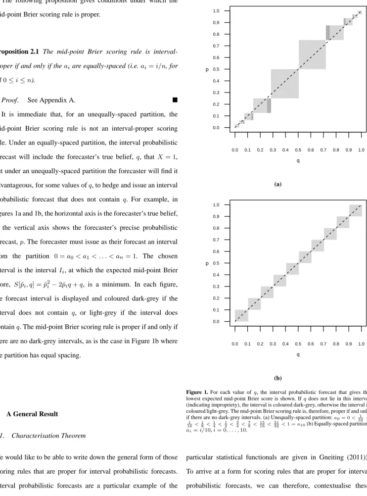
It is immediate that, for an unequally-spaced partition, the mid-point Brier scoring rule is not an interval-proper scoring rule. Under an equally-spaced partition, the interval probabilistic forecast will include the forecaster’s true belief,q, that X= 1, but under an unequally-spaced partition the forecaster will find it advantageous, for some values ofq, to hedge and issue an interval probabilistic forecast that does not contain q. For example, in figures 1a and 1b, the horizontal axis is the forecaster’s true belief,
q; the vertical axis shows the forecaster’s precise probabilistic forecast,p. The forecaster must issue as their forecast an interval from the partition 0 =a0< a1< . . . < an= 1. The chosen
interval is the intervalIi, at which the expected mid-point Brier
score, S[ˆpi, q] = ˆpi2−2ˆpiq+q, is a minimum. In each figure,
the forecast interval is displayed and coloured dark-grey if the interval does not contain q, or light-grey if the interval does containq. The mid-point Brier scoring rule is proper if and only if there are no dark-grey intervals, as is the case in Figure 1b where the partition has equal spacing.
3. A General Result
3.1. Characterisation Theorem
We would like to be able to write down the general form of those scoring rules that are proper for interval probabilistic forecasts. Interval probabilistic forecasts are a particular example of the wider class of statistical functionals (see for example, Gneiting 2011). Recently, Lambert et al. (2008); Lambert and Shoham (2009); Lambert (2013) and Frongillo and Kash (2014) have derived a general expression for scoring rules that are proper for statistical functionals (scoring rules that are proper for some
0.0 0.1 0.2 0.3 0.4 0.5 0.6 0.7 0.8 0.9 1.0 0.0 0.1 0.2 0.3 0.4 0.5 0.6 0.7 0.8 0.9 1.0 p q (a) 0.0 0.1 0.2 0.3 0.4 0.5 0.6 0.7 0.8 0.9 1.0 0.0 0.1 0.2 0.3 0.4 0.5 0.6 0.7 0.8 0.9 1.0 p q (b)
Figure 1. For each value ofq, the interval probabilistic forecast that gives the lowest expected mid-point Brier score is shown. Ifqdoes not lie in this interval (indicating impropriety), the interval is coloured dark-grey, otherwise the interval is coloured light-grey. The mid-point Brier scoring rule is, therefore, proper if and only if there are no dark-grey intervals. (a) Unequally-spaced partition:a0= 0< 1
32< 1 16< 1 8 < 1 4< 1 2< 3 4< 7 8< 15 16< 31 32<1 =a10(b) Equally-spaced partition: ai=i/10,i= 0, . . . ,10.
particular statistical functionals are given in Gneiting (2011)). To arrive at a form for scoring rules that are proper for interval probabilistic forecasts, we can therefore, contextualise these general results, in particular those of Lambert (2013), to our setting. With this indirect approach, however, we risk being opaque. Moreover, for interval forecasts of a binary random variable, it is possible to give a straightforward derivation of the functional form that an interval-proper scoring rule must have,
and this we now do. The reader inclined more to application may move immediately to Theorem 3.1.
As in the previous section,Xis a random variable taking only the values 0 and 1, for which the forecaster issues an interval probabilistic forecast,Ii, for some0< i≤n. What is the general
expression for the strictly interval-proper scoring rules?
Recalling that the expected value of s(Ii, X) when the
probability thatX= 1isq, is defined by
s[Ii, q] =Eq[s(Ii, X)]
=s(Ii,0)(1−q) +s(Ii,1)q (1)
the propriety ofsgives
s[Ik, q]≤s
Ij, q
for allk, jandq∈Ik. (2)
The condition (2) must be satisfied for every q∈Ik and, in
particular, for q=ak. Therefore, letting j=k+ 1 and q=ak,
we have
s[Ik, ak]≤s[Ik+1, ak]. (3)
From the strict propriety ofs,
s[Ik+1, q]< s[Ik, q] ∀q∈Ik+1.
By equation (1), for eachi,s[Ii, q]is a continuous function ofq
(a reasonable property: a forecaster who changes their true belief,
q, by a small amount should not wish their expected score to change substantially). The continuity ofs[Ii, q]inqfor alligives,
in particular,limq→a+ j
s[Ii, q] =sIi, aj,∀i, j. This smoothness
condition coupled with strict propriety gives
s[Ik, ak] = lim q→a+ k s[Ik, q] ≥ lim q→a+ k s[Ik+1, q] =s[Ik+1, ak]. (4)
Consequently, from (3) and (4), we have
s[Ik, ak] =s[Ik+1, ak]. (5)
Using (1), equation (5) may be written as
s(Ik,0)−s(Ik+1,0) (1−ak)
+
s(Ik,1)−s(Ik+1,1) ak= 0 (6)
and this must hold for everyk= 1, . . . , n−1.
One possible solution to (6) is the trivial solutions(Ik, X) = 0
for all values of k and X. But such a solution violates the condition of strict propriety: suppose that i < j and choose
q∈Ii; by strict propriety we should haves[Ii, q]< sIj, q, but
becauses(Ik, X) = 0for allkandXwe haves[Ii, q] =s
Ij, q
, a contradiction. So, the trivial solution is inadmissible.
Excluding the trivial solution, for each k= 1, . . . , n−1, the solution must then have the form,
s(Ik,0)−s(Ik+1,0) =−akγk
s(Ik,1)−s(Ik+1,1) = (1−ak)γk (7)
whereγkis a constant. We now show thatγkis non-negative. For
k >1, from the propriety ofswe have thats[Ik, q]≤s[Ik+1, q]
for allq∈Ik= (ak−1, ak], which together with the smoothness
ofs, gives
s[Ik, ak−1] = lim q→a+ k−1 s[Ik, q] ≤ lim q→a+ k−1 s[Ik+1, q] =s[Ik+1, ak−1].
For k= 1, I1= [a0, a1] and the propriety of s alone gives s[I1, a0]≤s[I2, a0]. So, for allk,
s[Ik, ak−1]≤s[Ik+1, ak−1]. (8)
Applying (1) to s[Ik, ak−1] and s[Ik+1, ak−1] in (8) and rearranging the terms in the inequality,
s(Ik,0)−s(Ik+1,0) (1−ak−1)
+
s(Ik,1)−s(Ik+1,1) ak−1≤0.
Substituting from (7) gives
−akγk(1−ak−1) + (1−ak)γkak−1≤0
⇔ γk(ak−1−ak)≤0
⇔ γk ≥0.
We can, therefore, write
s(Ik, X)−s(Ik+1, X) =γk(X−ak)
fork= 1, . . . , n−1 (9)
for non-negative constantsγk. The difference equation (9) has a
solution s(Ik, X) =f(X)− k−1 X i=1 γi(X−ai) (10)
with f an arbitrary function of X. Defining the function g
by g(i)−g(i−1) =γi, i= 1, . . . , n−1, we have proved the
following theorem
Theorem 3.1 (Characterisation for Interval-Proper Scoring Rules) Let X∈ {0,1} be a future binary observation. Given a partition0 =a0< a1< . . . < an−1< an= 1, letsbe a strictly
interval-proper scoring rule for interval probabilistic forecasts
I1= [a0, a1]andIk = (ak−1, ak]fork= 2, . . . , nof the outcome
X= 1. Thenshas the form
s(Ik, X) =f(X)− k−1 X i=1 g(i)−g(i−1) (X−ai) (11)
where f is an arbitrary function and g is a non-decreasing function.
Note that undersgiven by equation (11), interval probabilistic forecasts that are closer to the outcome forXreceive a lower (that is, better) score than interval probabilistic forecasts that are further from the outcome forX. Suppose thatX= 0. We have
s(Ik,0) =f(0) + k−1 X i=1 g(i)−g(i−1) ai
and the summation term increases askincreases (gbeing a non-decreasing function) so that asIkmoves further away fromX(as
kincreases)s(Ik,0)increases. Similarly, ifX= 1,
s(Ik,1) =f(1)− k−1 X i=1 g(i)−g(i−1) (1−ai)
and the summation term is always positive and increases in size ask increases so thats(Ik,1)increases asIk moves away from
X(askdecreases).
3.2. Choosingfandg
In equation (11), each choice for the function f and for the non-decreasing functiong, will give a new proper scoring rule for interval probabilistic forecasts. How should the functionsfandg
be chosen? While any real-valued function may be chosen forf
and any non-decreasing real-valued function may be chosen for
g, it is helpful to have some method to guide these choices. Here we suggest one such method.
To begin, chooseξk∈Ik+1fork= 0, . . . , n−1and define the functionhbyh(ξk) =g(k). Replacinggbyhin (11),
s(Ik, X) =f(X)− k−1 X i=1 h(ξi)−h(ξi−1) (X−ai) (12) from which s(Ik+1, X)−s(Ik, X) = −(h(ξk)−h(ξk−1))(X−ak). (13)
Restrict attention to thoses for which, asnincreases and all subintervals of the partition are made steadily smaller, the value of
sfor the interval containingptends to the value of some precise-proper scoring ruleS atp. Then (see Appendix B), for suitably smooth functionsSandh, lettingn→ ∞in (13), gives
∂S(p, X)
∂p =
dh(p)
dp (p−X). (14)
So, if we have a scoring rule, S, that is proper for precise probabilistic forecasts, we substitute for this scoring rule into the left-hand side of (14) and solve forhas a function ofp; having done so, we setg(k) =h(ξk)(for some predetermined choice for
theξk).
To interpreth, integrate both sides of (14) with respect topto obtain
S(p, X) +a(X) =h(p)(p−X)−
Z
h(p)dp
wherea(·)is a function ofXalone. Taking the expectation in
Xunderpgives
S[p, p] +Ep[a(X)] =−
Z
h(p)dp.
WithX∈ {0,1}, we can writea(X) =a(0)(1−X) +a(1)X
so that Ep[a(X)] =a(0)(1−p) +a(1)p. The function eS(p) =
−S[p, p]is known as the entropy ofpassociated withS(Gneiting and Raftery 2007; Br¨ocker 2009). We have
Z
h(p)dp= eS(p)−a(0)(1−p)−a(1)p
from which, differentiating both sides with respect top,
h(p) = deS(p)
dp −(a(1)−a(0)). (15)
Equation (15) states that h(p) is (up to a constant), the derivative of the entropy of p associated with S (we thank an anonymous referee for bringing this property ofhto our attention and for suggesting that this property ofhpromises an interesting form for equation (12) in the limit, a form which we resolve in the next paragraph).
Lead by this interpretation ofh, from equation (12), we have (where the indicator function1(·)has the value1if its argument is true, and0otherwise)
s(Ik, X) =f(X)− k−1 X i=1 h(ξi)−h(ξi−1) (X−ai) =f(X)− n X i=1 (X−ai)1(ai< ak) h(ξi)−h(ξi−1) . (16)
Allowingn→ ∞in equation (16), we obtain
S(p, X) =f(X)−
Z
(X−q)1(q < p)dh(q) (17)
which (for our choice of f, see below) is the Schervish-representation of a proper scoring rule for a binary event (Schervish (1989),Theorem 4.2,page 1861; see also Gneiting and Raftery (2007), page 364).
What of the functionf? From equation (11) we have that
s(I1, X) =f(X)
We choose f(X) =S(ξ0, X). This choice ensures that
s(I1, X)→S(0, X)asn→ ∞.
As examples of this method we take some familiar precise-proper scoring rules and derive the corresponding analogues that are interval-proper. In all cases, we assume thatXtakes only the values0 and 1, the precise probabilistic forecast that X= 1 is
pand that the interval [0,1]has n subintervals with end-points
0 =a0< a1< . . . < an= 1.
EXAMPLE (Brier scoring rule (Brier 1950)). The Brier scoring rule isS(p, X) = (p−X)2. Substituting forS in (14), we have
−2(X−p) = (p−X)dh(p) dp
giving h(p) = 2p. Identify points ξk∈Ik+1 for all
k= 0, . . . , n−1. Then g(k) =h(ξk) = 2ξk. Choose
f(X) = (ξ0−X)2.
With these choices offandg, equation (11) gives the following Brier scoring rule for interval probabilistic forecasts
s(Ik, X) = (ξ0−X)2−
k−1
X
i=1
(2ξi−2ξi−1) (X−ai)
which may be rewritten as
s(Ik, X) = (ξk−1−X)2− k−1 X i=1 n (ξi−ai)2−(ξi−1−ai)2 o (18)
and the expected interval Brier score is
s[Ik, q] =q−2qξk−1+ξ 2 k−1 − k−1 X i=1 n (ξi−ai)2−(ξi−1−ai)2 o .
If we choose ξk=12(ak+ak+1), the mid-point of each subinterval, then s(Ik, X) = 1 2(ak−1+ak)−X 2 −1 4(ak−ak−1) 2+1 4a 2 1 (19) =(X−ak−1)(X−ak) + 1 4a 2 1. (20)
Since propriety is preserved under translation, we define the adjusted interval-proper Brier scoring rule by
s(Ik, X) = (X−ak−1)(X−ak). (21)
Equation (19) also shows that whenξkis the mid-point of the
(k+ 1)st interval, then, under equally-spaced subintervals,
s(Ik, X) =
1
2(ak−1+ak)−X
2
which, from Proposition 2.1, is known to be proper.
✷ EXAMPLE (Ignorance scoring rule (Good 1952)). The Ignorance scoring rule is defined by
S(p, X) =−Xlog(p)−(1−X) log(1−p) forp∈(0,1). Substituting into (14) gives
p−X
p(1−p) = (p−X)
dh(p)
dp .
We have, therefore, that forp∈(0,1),h(p) = log{p/(1−p)}, from which g(k) =h(ξk) = log{ξk/(1−ξk)}, for 0≤k < n.
Choosef(X) =S(ξ0, X).
The expression fors(Ik, X)may be written
s(Ik, X) =S(ξk−1, X)−
k−1
X
i=1
{S(ξi, ai)−S(ξi−1, ai)}
which is of the same form as equation (18) for the Brier scoring rule, although, for the ignorance scoring rule there is no apparent simplification similar to that by which equation (18) reduces to equation (20) for the Brier scoring rule.
✷ EXAMPLE(Pseudo-spherical scoring rule (Roby 1964)). Fix
α >1. Theα-pseudo-spherical scoring rule is
S(p, X) ={−Xp+ (X−1)(1−p)}
α−1
{pα+ (1−p)α}α−1 α
. c 0000 Royal Meteorological Society qjrms4.cls
ReplacingSin (14) gives dh(p) dp = (α−1){(p−1)p}α−2 {pα+ (1−p)α}2−1 α .
Solving forh, we have
h(p) = p
α−1−(1−p)α−1
{pα+ (1−p)α}α−1 α
.
Set g(k) =h(ξk) and choose f(X) =S(ξ0, X). (If α= 2, the pseudo-spherical scoring rule is referred to as the spherical scoring rule.)
✷
4. Consequences of Impropriety
Equation (11) presents the characteristic form that an interval-proper scoring rule must have. Yet it is unclear what the practical implications are if an improper interval scoring rule is used. In this section, we use actual precise probabilistic forecasts provided by two separate meteorological offices to construct hypothetical interval probabilistic forecasts when an improper interval scoring rule is in place. From these synthetic, yet representative, interval probabilistic forecasts, we can establish empirical measures of the influence of impropriety.
4.1. Data
Two separate data sets, in both cases precipitation data, were used. The amount of precipitation per day (the 24-hour period beginning at midnight local time) is converted into a binary variable,X, by choosing a threshold rainfall level (in mm) and definingX = 1if the recorded amount of precipitation is greater than or equal to the threshold level; otherwiseX= 0.
The UK Meteorological Office (UKMO) provided data for 58 lead-times (from 6 to 348 hours at 6-hourly intervals) and 2locations; for each lead-time and location pair approximately two-years of daily data was available. For each day of each lead-time and location pair, the observation was a precipitation level (in mm) and the forecast was given as a set of nodes
(zj, F(zj))j= 1, . . . , mof the cumulative distribution function
(F) of the precipitation level in mm (z), from which the precise probability of the precipitation level exceeding a threshold of1mm was calculated; if necessary, the nodes were linearly interpolated and the tails were linearly extrapolated, that is, the upper limit of the cumulative distribution function was determined by
z∗= 1−F(zm) F(zm)−F(zm−1) (zm−zm−1) +zm
and the lower limit of the cumulative distribution function was calculated as z∗= max 0, z1− F(z1)−0 F(z2)−F(z1) (z2−z1) .
UKMO precise probabilistic forecasts were translated into interval probabilistic forecasts (see below) using the following partition of the interval[0,1]used by the UKMO:a0= 0,0.025, 0.05, 0.10, 0.20, 0.25, 0.30, 0.40, 0.50, 0.60, 0.70, 0.75, 0.80, 0.90,0.95,1 =a15.
The Australian Bureau of Meteorology (ABOM) computes precise probabilistic forecasts for X based on a threshold level of 0.2mm. For each day, a total of 7 different forecasts are computed: a forecast being calculated at 12, 36, 60, 84, 108, 132 and 156 hours before the start of the day to which the recorded precipitation amount refers. The data consisted of the7 precise probabilistic forecasts for each of290consecutive days for 18different locations around Australia; missing data (either observed precipitation or precise probabilistic forecast) was omitted not imputed. The ABOM precise probabilistic forecasts were converted to interval probabilistic forecasts (see below) using the following partition of the interval[0,1]:a0= 0,0.025, 0.075,0.15,0.25,0.35,0.45,0.55,0.65,0.75,0.85,0.925,0.975, 1 =a13; this partition is used by the ABOM.
4.2. Calculating Interval Probabilistic forecasts
The data described in the previous subsection are precise probabilistic forecasts. We now describe how these data may be used to calculate interval probabilistic forecasts. We begin
by assuming that each precise probabilistic forecast, p, is determined under a precise-proper scoring rule and so represents the forecaster’s true belief that X= 1. Next, suppose that the forecaster is made aware of both the interval scoring rule,s, by which they will be evaluated (see for example, Gneiting (2011) on the need for the forecaster to be made aware of the scoring rule) and the partition 0 =a0< a1< . . . < an−1< an = 1
from which they must choose an interval. The interval chosen by the forecaster, Ik, is that which optimises their expected
score,s[Ik, p]. Ifsis an interval-proper scoring rule, the interval
issued by the forecaster will be the interval containingp. Under an interval-improper scoring rule, the forecast interval will not necessarily contain the forecaster’s true beliefp.
In this manner, for each precise probabilistic forecast in the data two interval probabilistic forecasts are computed: one whens is an interval-improper scoring rule and one when sis an interval-proper scoring rule. We emphasise that all interval probabilistic forecasts so calculated are hypothetical and are not actual interval probabilistic forecasts provided by either the UKMO or the ABOM.
4.3. Skill
Let xi be the ith recorded binary observation and Iki be
the interval probabilistic forecast associated with xi, i=
1, . . . , N. The forecaster’s accuracy is their average score¯sN =
1
N
PN
i=1s(Iki, xi). In the limit, the forecaster’s average score is
the expected valueE[s(I, X)], where the expected value is taken over the joint distribution of the intervalsIand the observationX. For largeN,s¯Nis approximately normally distributed with mean
E[s(I, X)]and varianceσˆ2/Nwhere
ˆ σ2= 1 N−1 N X i=1 s(Iki, xi)−s¯N 2
A forecaster’s skill is evaluated by comparing their accuracy to the accuracy of other forecasters; specifically, we make comparisons with the accuracy of the perfect forecaster and the accuracy of the climatological forecaster. The climatological forecaster computes their actual precise belief from the
distribution of precipitation over some agreed historical period. (The UKMO historical period is 1983-2012, and the ABOM historical period is 1981-2010. Both the UKMO and the ABOM provide site-specific climatological probabilistic forecasts as a set of nodes(zj, Fclim(zj))forj= 1, . . . , mclimfrom which the precise climatological forecast is calculated as the probability of exceeding the applicable threshold; linear interpolation and extrapolation are used where necessary in the manner described above.)
We define (Wilks 2006, page 259), the forecaster’s skill by
E[s(I, X)]−Eclim[s(I, X)] Eperf[s(I, X)]−Eclim[s(I, X)]
(22)
whereµclim=Eclim[s(I, X)]is the accuracy of the climato-logical forecaster andµperf=Eperf[s(I, X)]is the accuracy of the perfect forecaster, from which, taking µclim and µperf as constant, a forecaster’s skill is approximately normally distributed with mean E[s(I, X)]−µclim µperf−µclim and variance ˆ σ2 N µperf−µclim 2
A skill of 1 for a forecaster demonstrates a perfect forecast record for the forecaster, while a skill of 0 indicates that the forecaster is no more skillful than a climatological forecaster.
EXAMPLE(Brier scoring rule (Brier 1950)). Let0 =a0<
a1< . . . < an= 1 be a partition of unequally-spaced intervals.
Chooseξkto be the mid-point ofIk+1for eachk= 0, . . . , n−1. Letsbe the adjusted interval-proper Brier scoring rule (equation (21)) and s˜be the interval-improper adjusted mid-point Brier scoring rule ˜ s(Ik, X) = (ξk−1−X) 2 −1 4a 2 1 = (X−ak−1)(X−ak) +1 4(ak−ak−1) 2−1 4a 2 1 (23)
(For equally-spaced intervalssands˜are equivalent; but, here, unequally-spaced intervals are supposed.)
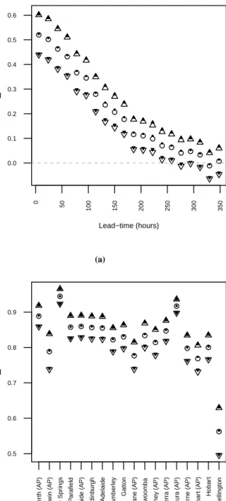
Figures 2a and 2b compare forecaster skill under s (proper) ands˜(improper). In figure 2a, the skill of interval probabilistic forecasts at Heathrow Airport for different lead-times is shown. In figure 2b, the skill of the12-hour lead-time forecast at each of 18different locations around Australia is plotted.
✷ The immediate conclusion from the above example is that there appears to be no material difference in skill measured under the interval-proper and interval-improper (Brier) scoring rules.
But, there is a more insidious danger from impropriety: impropriety permits hedging, wherein the forecaster chooses to publish an interval probabilistic forecast that differs from the interval they truly believe is appropriate. In such cases, a forecaster’s accuracy (or skill) does not measure their true forecasts but measures their given forecasts, thereby misrepresenting their ability. In the presence of hedging, decisions based on the forecaster’s ability, in particular whether one forecaster is better than another, are invalid.
For a given interval-improper scoring rule, ˜s, and the forecaster’s true (precise) belief that X= 1, q, whether a forecaster is induced to hedge depends on the values of ˜s[I, q] for different intervalsI, and therefore, only on the partition from which the interval forecasts are selected. In the example that follows we demonstrate the effect of the choice of partition on a forecaster’s hedging profile.
EXAMPLE(Brier scoring rule (Brier 1950) cont.). Assume unequally-spaced intervals and the interval-improper adjusted mid-point Brier scoring rule given by equation (23). We consider the interval probabilistic forecasts issued at Heathrow and Perth Airports. 0 50 100 150 200 250 300 350 0.0 0.1 0.2 0.3 0.4 0.5 0.6 Lead−time (hours) Skill (a) 0.5 0.6 0.7 0.8 0.9 Skill P er th (AP)
Darwin (AP) Alice Spr
ings P ar afield Adelaide (AP) Edinb urgh Adelaide Amber le y Gatton Br isbane (AP) Too w oomba Sydne y (AP) Canberr a (AP) Mildur a (AP) Melbour ne (AP) Hobar t (AP) Hobar t Mt W ellington (b)
Figure 2. In each figure, estimated forecaster skill (defined by equation (22)) and
95% confidence intervals are shown under the adjusted interval-proper Brier scoring rule (◭ • ◮) and the interval-improper adjusted mid-point Brier scoring rule (⊳ ◦ ⊲). (a) Skill of interval probabilistic forecasts at Heathrow Airport for different forecast lead-times. (b) Skill of interval probabilistic forecasts for the12 -hour lead-time at different locations in Australia.
In the bar-graphs below, the height of each bar is the proportion of times the interval is issued as a forecast. For each bar, the white area (if any) is the proportion of times the interval is forecast and is a hedge that understates the forecaster’s true belief; the dark-grey area (if any) is the proportion of times the interval is forecast and is a hedge that overstates the forecaster’s true belief. (In all cases, an understated forecast is a forecast of the interval immediately below the true interval forecast and an overstated
forecast is a forecast of the interval immediately above the true interval forecast.) The points marked by•, are the proportion of times the interval is a hedge given the interval is forecast, that is, the propensity to hedge.
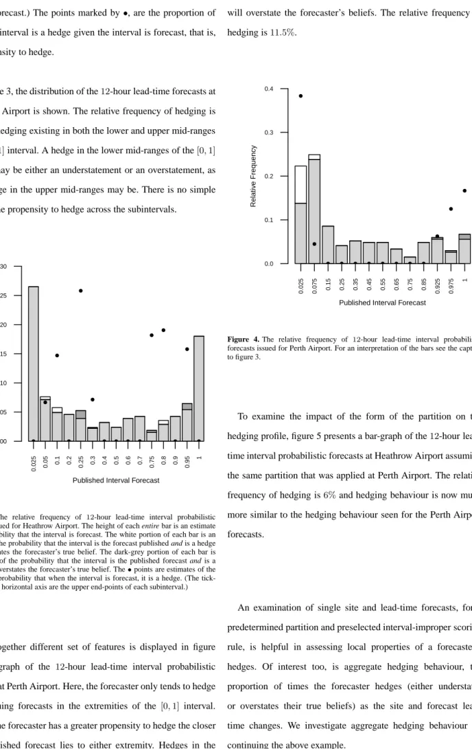
In figure 3, the distribution of the12-hour lead-time forecasts at Heathrow Airport is shown. The relative frequency of hedging is 5%with hedging existing in both the lower and upper mid-ranges of the[0,1]interval. A hedge in the lower mid-ranges of the[0,1] interval may be either an understatement or an overstatement, as too a hedge in the upper mid-ranges may be. There is no simple trend in the propensity to hedge across the subintervals.
0.025 0.05 0.1 0.2 0.25 0.3 0.4 0.5 0.6 0.7 0.75 0.8 0.9 0.95 1 0.00 0.05 0.10 0.15 0.20 0.25 0.30
Published Interval Forecast
Relativ
e Frequency
Figure 3. The relative frequency of 12-hour lead-time interval probabilistic forecasts issued for Heathrow Airport. The height of each entire bar is an estimate of the probability that the interval is forecast. The white portion of each bar is an estimate of the probability that the interval is the forecast published and is a hedge that understates the forecaster’s true belief. The dark-grey portion of each bar is an estimate of the probability that the interval is the published forecast and is a hedge that overstates the forecaster’s true belief. The•points are estimates of the conditional probability that when the interval is forecast, it is a hedge. (The tick-labels on the horizontal axis are the upper end-points of each subinterval.)
An altogether different set of features is displayed in figure 4, a bar-graph of the 12-hour lead-time interval probabilistic forecasts at Perth Airport. Here, the forecaster only tends to hedge when issuing forecasts in the extremities of the [0,1] interval. Further, the forecaster has a greater propensity to hedge the closer their published forecast lies to either extremity. Hedges in the lower ranges of the[0,1]interval will understate the forecaster’s
beliefs while hedges in the upper ranges of the [0,1] interval will overstate the forecaster’s beliefs. The relative frequency of hedging is11.5%. 0.025 0.075 0.15 0.25 0.35 0.45 0.55 0.65 0.75 0.85 0.925 0.975 1 0.0 0.1 0.2 0.3 0.4
Published Interval Forecast
Relativ
e Frequency
Figure 4. The relative frequency of 12-hour lead-time interval probabilistic forecasts issued for Perth Airport. For an interpretation of the bars see the caption to figure 3.
To examine the impact of the form of the partition on the hedging profile, figure 5 presents a bar-graph of the12-hour lead-time interval probabilistic forecasts at Heathrow Airport assuming the same partition that was applied at Perth Airport. The relative frequency of hedging is6%and hedging behaviour is now much more similar to the hedging behaviour seen for the Perth Airport forecasts.
✷ An examination of single site and lead-time forecasts, for a predetermined partition and preselected interval-improper scoring rule, is helpful in assessing local properties of a forecaster’s hedges. Of interest too, is aggregate hedging behaviour, the proportion of times the forecaster hedges (either understates or overstates their true beliefs) as the site and forecast lead-time changes. We investigate aggregate hedging behaviour by continuing the above example.
0.025 0.075 0.15 0.25 0.35 0.45 0.55 0.65 0.75 0.85 0.925 0.975 1 0.00 0.05 0.10 0.15 0.20 0.25 0.30
Published Interval Forecast
Relativ
e Frequency
Figure 5. The relative frequency of 12-hour lead-time interval probabilistic forecasts issued for Heathrow Airport under the same partition used for the forecasts issued for Perth Airport in figure 4. For an interpretation of the bars see the caption to figure 3.
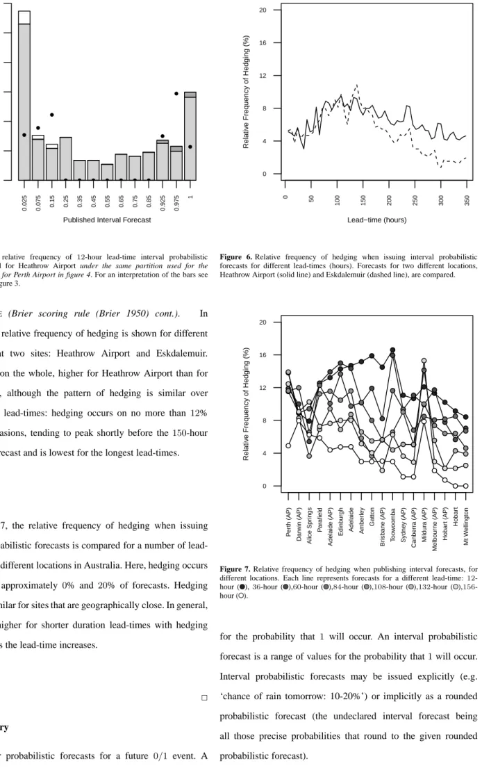
EXAMPLE (Brier scoring rule (Brier 1950) cont.). In figure 6, the relative frequency of hedging is shown for different lead-times at two sites: Heathrow Airport and Eskdalemuir. Hedging is, on the whole, higher for Heathrow Airport than for Eskdalemuir, although the pattern of hedging is similar over the different lead-times: hedging occurs on no more than 12% or so of occasions, tending to peak shortly before the150-hour lead-time forecast and is lowest for the longest lead-times.
In figure 7, the relative frequency of hedging when issuing interval probabilistic forecasts is compared for a number of lead-times across different locations in Australia. Here, hedging occurs on between approximately 0% and 20% of forecasts. Hedging levels are similar for sites that are geographically close. In general, hedging is higher for shorter duration lead-times with hedging decreasing as the lead-time increases.
✷
5. Summary
We consider probabilistic forecasts for a future 0/1 event. A precise probabilistic forecast is a statement of the exact value
0 50 100 150 200 250 300 350 0 4 8 12 16 20 Lead−time (hours) Relativ e Frequency of Hedging (%)
Figure 6. Relative frequency of hedging when issuing interval probabilistic
forecasts for different lead-times (hours). Forecasts for two different locations, Heathrow Airport (solid line) and Eskdalemuir (dashed line), are compared.
0 4 8 12 16 20 P er th (AP)
Darwin (AP) Alice Spr
ings P ar afield Adelaide (AP) Edinb urgh Adelaide Amber le y Gatton Br isbane (AP) Too w oomba Sydne y (AP) Canberr a (AP) Mildur a (AP) Melbour ne (AP) Hobar t (AP) Hobar t Mt W ellington Relativ e Frequency of Hedging (%)
Figure 7. Relative frequency of hedging when publishing interval forecasts, for
different locations. Each line represents forecasts for a different lead-time:12 -hour ( ),36-hour ( ),60-hour ( ),84-hour ( ),108-hour ( ),132-hour ( ),156 -hour ( ).
for the probability that 1 will occur. An interval probabilistic forecast is a range of values for the probability that1will occur. Interval probabilistic forecasts may be issued explicitly (e.g. ‘chance of rain tomorrow: 10-20%’) or implicitly as a rounded probabilistic forecast (the undeclared interval forecast being all those precise probabilities that round to the given rounded probabilistic forecast).
Probabilistic forecasts must be evaluated using proper scoring rules. Scoring rules that are proper when the forecast probability is a precise value are not, in general, proper when applied to a representative probability from the interval forecast. Analogous to the result of Lambert (2013), we present a general expression for scoring rules that are proper for interval probabilistic forecasts. Specific interval-proper scoring rules, corresponding to the more familiar precise-proper scoring rules (Brier scoring rule, Ignorance scoring rule and Pseudo-spherical scoring rule) are also given; of these, the interval-proper Brier scoring rule (equation (21)) has a simple and appealing form.
The importance of interval-proper scoring rules is their use in assessing the performance of forecasters issuing interval probabilistic forecasts. That is not to say that an interval-improper scoring rule necessarily results in a meaningful change in a forecaster’s calculated skill; substituting an interval-improper scoring rule for an interval-proper scoring rule can have little quantifiable impact on a forecaster’s skill. Rather, the egregious effect of impropriety is on the interpretation of a forecaster’s computed skill. Under impropriety, a forecaster may hedge when issuing a forecast, giving a forecast that does not reflect their true opinion. In such cases the skill, being based on the published forecasts, no longer represents the forecaster’s true views and gives only partial insight into their substantive ability.
We calculate the relative frequency of hedging using interval probabilistic forecasts simulated using precise probability of precipitation (PoP) forecasts provided by The Australian Bureau of Meteorology and the UK Meteorological Office. While hedging varies with site and forecast lead-time, the relative frequency of hedging in the cases we consider lies approximately in the range of0−15%.
Interval-proper scoring rules depend explicitly on the set of intervals to which the interval forecasts refer. A change of the intervals used to express forecasts will influence the scoring rule and a natural question arises as to whether there is an optimal set of intervals. The question may be framed as a high-dimensional non-linear constrained optimisation problem and while we have
not conducted a general investigation of this problem, in the particular case of the unadjusted interval-proper Brier scoring rule (equation (20)) it can be shown that the optimal partition is the equally-spaced partition, when ‘optimal’ is defined as the interval-proper Brier scoring rule being close in the squared-error sense to the precise-proper Brier scoring rule.
Acknowledgements
We would like to thank Prof. A. Abu-Hanna for introducing us to the problem of proper scoring rules for interval probabilistic forecasts. For their generous help in providing the data used in this paper, we would like to thank the Australian Burerau of Meteorology, in particular, Dr. D. Griffiths and Ms. I. Ioannou, and the UK Meteorological Office, specifically Dr. M. Mittermaier. Lastly, to the two anonymous referees, for their comments and suggestions, our sincerest thanks.
A. Appendix
For 0< i≤n, write pˆi=21(ai−1+ai), the mid-point of the
intervalIi. The mid-point Brier scoring rule is defined by
s(Ii, X) = (ˆpi−X)2
and satisfies s[Ii, q] =Eq[s(Ii, X)] = ˆp2i −2ˆpiq+q. The
mid-point Brier scoring rule is interval-proper if and only if
s[Ii, q]≤sIj, q ∀i, j and∀q∈Ii.
Proof of Proposition 2.1: the mid-point Brier scoring rule is proper if and only if the partition is equally-spaced.
Proof. Suppose that the mid-point Brier scoring rule is interval-proper. Then
s[Ii, q]≤sIj, q ∀i, j and∀q∈Ii
which holds if and only if, fixingi,∀q∈Ii,
q≤1
4(ai−1+ai+aj−1+aj) i < j
q≥1
4(ai−1+ai+aj−1+aj) i > j. (24)
Condition (24) must hold for allq∈Iiand so holds forq=ai.
In this case, ai≤1 4(ai−1+ai+aj−1+aj) i < j and, lettingj=i+ 1, ai≤1 4(ai−1+ai+ai+ai+1) from which ai−ai−1≤ai+1−ai.
Also, condition (24) must hold for q= infIi=ai−1. Specifically, ai−1≥ 1 4(ai−1+ai+aj−1+aj) i > j. Lettingj=i−1, ai−1≥1 4(ai−1+ai+ai−2+ai−1) giving ai−1−ai−2≥ai−ai−1.
As i was fixed arbitrarily, we have, for all 0< i < n,
ai−ai−1≤ai+1−ai and for 1< i≤n, ai−1−ai−2≥
ai−ai−1.
Now, for any0< k < n, leti=k, to giveak+1−ak≥ak−
ak−1 and let i=k+ 1 to give ak−ak−1≥ak+1−ak, from
which
ak+1−ak=ak−ak−1
and this holds for all0< k < n, that is, theaiare equally-spaced.
Conversely, suppose that theai are equally-spaced; ai=i/n
for all0≤i≤n. Then
1 4(ai−1+ai+aj−1+aj) = 1 n i+j−1 2 . Ifi < jtheni≤j−1and ai=ni ≤ 1n i+j−1 2 = 1 4(ai−1+ai+aj−1+aj)
so q≤14(ai−1+ai+aj−1+aj) for all q∈Ii with i < j.
Equally, ifi > jtheni−1≥jand
ai−1= i−1 n ≥ 1 n i+j−1 2 =1 4(ai−1+ai+aj−1+aj) so thatq≥1
4(ai−1+ai+aj−1+aj) for allq∈Ii withi > j. Condition (24) is satisfied and therefore, the mid-point Brier scoring rule is interval-proper.
We remark in passing that the propriety of the more generalλ -Brier scoring rule, defined by s(Ii, X) ={(1−λ)ai−1+λai−
X}2also depends critically on the spacing of the partition, being proper if and only if, letting∆i=ai−ai−1,
∆1 ∆1+∆2 ≤ λ ≤ 1 forq∈I1 ∆k ∆k+∆k+1 ≤ λ ≤ ∆k−1 ∆k+∆k−1 forq∈Ik 1< k < n 0 ≤ λ ≤ ∆n−1 ∆n+∆n−1 for q∈In B. Appendix
We show under certain conditions on the partition0 =a0< a1<
. . . < an= 1, and on the functionss,Sandh, that, lettingξk∈
Ik+1, asnincreases the equation
s(Ik+1, X)−s(Ik, X) =
−(h(ξk)−h(ξk−1))(X−ak) (25)
leads to the differential equation
∂S(p, X)
∂p =
dh(p)
dp (p−X). (26)
Definition B.1 The partitions [a]n=an,0< an,1< . . . < an,n,
0 =an,0,1 =an,n, are said to be increasingly refined asn→ ∞
if the mesh,µn= max{an,i−an,i−1|i= 1, . . . , n}tends to0. Remark. When refering to subintervals of the partition
[a]n=an,0< an,1< . . . < an,n, 0 =an,0, 1 =an,n, we shall
use the notation In,1= [an,0, an,1], In,k= (an,k−1, an,k] for
k= 2, . . . , n.
Lemma B.1 Letp∈[0,1]. If the partitions[a]nare increasingly
refined then∀ǫ >0,∃N≥0such that for eachn > N, there is a k(depending onn) such that|an,k−p|< ǫ.
Proof. Fixǫ >0. Since the partitions[a]n are increasingly
refined, there is anN≥0such that∀n > N,µn< ǫ. Letn > N
so thatµn< ǫ. Ifp∈[0,1]then there is someksuch thatp∈In,k.
Therefore,|an,k−p| ≤ |an,k−an,k−1| ≤µn< ǫ. So for alln >
N, there exists ak(depending onn) such that|an,k−p|< ǫ.
Definition B.2 We shall say that the interval scoring rule s converges in the Lipschitz sense to the precise scoring rule S at p if and only if ∀ǫ >0, ∃N≥0 such that for all n≥N,
|s(In,k, x)−S(p, x)|< ǫmin{|an,k−1−p|,|an,k−p|}for allx,
p∈In,k. If s converges to S in the Lipschitz sense at every
p∈[0,1], then we shall say simply that sconverges toS in the Lipschitz sense.
Proposition B.1 Let s be an interval-proper scoring rule satisfying equation (25), with h continuously differentiable. Suppose that s converges to the precise scoring rule S in the Lipschitz sense, whereS is continuously partially differentiable with respect top. If the partitions [a]n are increasingly refined
then
∂S(p, X)
∂p =
dh(p)
dp (p−X).
Proof. Let ǫ >0, p∈[0,1]. S is continuously partially differentiable with respect top, so∃δ∗>0such that∀|r|< δ∗,
S(p+r, X)−S(p, X) r − ∂S(p, X) ∂p < ǫ 4
and∃δ′>0such that if|ξ−p|< δ′,
∂S(ξ, X) ∂ξ − ∂S(p, X) ∂p < ǫ 4.
Further, sincehis continuously differentiable,∃δ∗∗ such that
∀|r|< δ∗∗, h(p+r)−h(p) r − dh(p) dp < ǫ 2
and∃δ′′>0such that if|ξ−p|< δ′′, then
dh(ξ) dξ − dh(p) dp < ǫ 2. Letδ= min{δ∗, δ′, δ∗∗, δ′′, ǫ}.
As the partitions[a]n are increasingly refined,∃N∗≥0such
that forn≥N∗,µn<δ2. The interval scoring rulesconverges to Sin the Lipschitz sense, so∃N′≥0such that∀n > N′,
|s(In,j, X)−S(p, X)|<
ǫ
4min{|an,j−1−p|,|an,j−p|}
forp∈In,j. LetN= max{N∗, N′},n≥Nand letk(depending
onn) satisfyp∈In,k. From equation (25),
s(In,k+1, X)−s(In,k, X) ξn,k−ξn,k−1 = − h(ξ n,k)−h(ξn,k−1) ξn,k−ξn,k−1 (X−an,k) (27) where, as above,ξn,k∈In,k+1.
Considering the left-hand side of equation (27),
s(In,k+1, X)−s(In,k, X) ξn,k−ξn,k−1 −∂S(p, X) ∂p = s(In,k+1, X)−S(ξn,k, X) ξn,k−ξn,k−1 −s(In,k, X) +S(ξn,k−1, X) ξn,k−ξn,k−1 +S(ξn,k, X)−S(ξn,k−1, X) ξn,k−ξn,k−1 −∂S(ξn,k−1, X) ∂ξn,k−1 +∂S(ξn,k−1, X) ∂ξn,k−1 −∂S(p, X) ∂p ≤ s(In,k+1, X)−S(ξn,k, X) ξn,k−ξn,k−1 + s(In,k, X) +S(ξn,k−1, X) ξn,k−ξn,k−1 + S(ξn,k, X)−S(ξn,k−1, X) ξn,k−ξn,k−1 −∂S(ξn,k−1, X) ∂ξn,k−1 + ∂S(ξn,k−1, X) ∂ξn,k−1 −∂S(p, X) ∂p .
But,S is partially continuously differentiable with respect to
p,ξn,k−ξn,k−1≤an,k+1−an,k−1≤2µn< δ, and |ξn,k−1−
p|< µn< δ, from which it follows that
s(In,k+1, X)−s(In,k, X) ξn,k−ξn,k−1 −∂S(p, X) ∂p <ǫ 4 min{|an,k+1−ξn,k|,|an,k−ξn,k|} ξn,k−ξn,k−1 +ǫ 4 min{|an,k−ξn,k−1|,|an,k−1−ξn,k−1|} ξn,k−ξn,k−1 +ǫ 4+ ǫ 4 <ǫ 4+ ǫ 4+ ǫ 4+ ǫ 4 =ǫ
having noted too that
min{|an,k+1−ξn,k|,|an,k−ξn,k|} ξn,k−ξn,k−1 ≤ |an,k−ξn,k| ξn,k−ξn,k−1 ≤1 and, similarly min{|an,k−ξn,k−1|,|an,k−1−ξn,k−1|} ξn,k−ξn,k−1 ≤ |an,k−ξn,k−1| ξn,k−ξn,k−1 ≤1. Next, h(ξn,k)−h(ξn,k−1) ξn,k−ξn,k−1 −dh(p) dp = h(ξn,k)−h(ξn,k−1) ξn,k−ξn,k−1 −dh(ξn,k−1) dξn,k−1 +dh(ξn,k−1) dξn,k−1 −dh(p) dp ≤ h(ξn,k)−h(ξn,k−1) ξn,k−ξn,k−1 −dh(ξn,k−1) dξn,k−1 + dh(ξn,k−1) dξn,k−1 −dh(p) dp <ǫ 2+ ǫ 2 =ǫ. Finally, |(X−an,k)−(X−p)|=|p−an,k| ≤µn< δ2≤ǫ. Combining these separate limit results, equation (27) gives
∂S(p, X) ∂p =− dh(p) dp (X−p). References
Brier G. 1950. Verification of forecasts expressed in terms of probability. Monthly Weather Review 78(1): 1–3.
Br¨ocker J. 2009. Reliability, sufficiency, and the decomposition of proper scores. Quarterly Journal of the Royal Meteorological Society 135: 1512–1519. Dawid A. 1986. Probability forecasting. In: Encyclopedia of Statistical Sciences,
vol. 7, Kotz S, Johnson N, Read C (eds), John Wiley & Sons, pp. 210–218. Frongillo R, Kash I. 2014. General truthfulness characterizations via convex
analysis. ArXiv:1211.3043v3.
Gneiting T. 2011. Making and evaluating point forecasts. Journal of the American Statistical Association 106: 746–762.
Gneiting T, Katzfuss M. 2014. Probabilistic forecasting. Annual Review of Statistics and Its Application 2014(1): 125–151.
Gneiting T, Raftery A. 2007. Strictly proper scoring rules, prediction and estimation. American Statistical Association 102: 359–378.
Good I. 1952. Rational decisions. Journal of the Royal Statistical Society. Series B (Methodological) 14(1): 107–114.
Lambert N. 2013. Elicitation and evaluation of sta-tistical forecasts. Preprint. Stanford University. (web.stanford.edu/˜nlambert/papers/elicitation.pdf).
Lambert N, Pennock D, Shoham Y. 2008. Eliciting properties of probability distributions. EC ’08 Proceedings of the 9th ACM Conference on Electronic Commerce : 129–138.
Lambert N, Shoham Y. 2009. Eliciting truthful answers to multiple-choice questions. EC ’09 Proceedings of the 10th ACM Conference on Electronic Commerce : 109–118.
Murphy A. 1998. The early history of probability forecasts: Some extensions and clarifications. Weather and Forecasting 13: 5–15.
Murphy A, Epstein E. 1967. A note on probability forecasts and ‘hedging’. Journal of Applied Meteorology 6: 1002–1004.
Roby T. 1964. Belief states: A preliminary empirical study. Technical documentary report no. esd-tdr-64-238, Decision Sciences Laboratory, Electronic Systems Division, Air Force Systems Command, United States Air Force.
Schervish M. 1989. A general method for comparing probability assessors. The Annals of Statistics 17(4): 1856–1879.
Wilks D. 2006. Statistical methods in the atmospheric sciences. Elsevier, second edn.
Winkler R. 1996. Scoring rules and the evaluation of probabilities. Test 5(1): 1–60. Winkler R, Murphy A. 1968. ‘Good’ probability assessors. Journal of Applied
Meteorology 7: 751–758.