2016
Intrusion detection using probabilistic graphical
models
Liyuan Xiao
Iowa State UniversityFollow this and additional works at:
https://lib.dr.iastate.edu/etd
Part of the
Computer Sciences Commons
This Dissertation is brought to you for free and open access by the Iowa State University Capstones, Theses and Dissertations at Iowa State University Digital Repository. It has been accepted for inclusion in Graduate Theses and Dissertations by an authorized administrator of Iowa State University Digital Repository. For more information, please [email protected].
Recommended Citation
Xiao, Liyuan, "Intrusion detection using probabilistic graphical models" (2016).Graduate Theses and Dissertations. 16041.
by
Liyuan Xiao
A dissertation submitted to the graduate faculty in partial fulfillment of the requirements for the degree of
DOCTOR OF PHILOSOPHY
Major: Computer Science
Program of Study Committee: Carl K. Chang, Major Professor
Ying Cai Hailiang Liu Simanta Mitra Johnny S. Wong
Iowa State University Ames, Iowa
2016
TABLE OF CONTENTS
LIST OF TABLES . . . iv
LIST OF FIGURES . . . v
ACKNOWLEDGEMENTS . . . vii
CHAPTER 1. GENERAL INTRODUCTION . . . 1
CHAPTER 2. BAYESIAN MODEL AVERAGING OF BAYESIAN NET-WORK CLASSIFIERS FOR INTRUSION DETECTION . . . 6
2.1 Introduction . . . 7
2.2 Bayesian Networks and Bayesian Model Averaging . . . 9
2.2.1 Bayesian Network Classifier . . . 9
2.2.2 Bayesian Model Averaging of Bayesian Network Classifiers . . . 11
2.2.3 Finding thek-best Bayesian Network Structures . . . 13
2.3 Description of NSL-KDD Dataset . . . 14
2.4 Construction and Evaluation of BNMA Classifier . . . 14
2.4.1 Feature Selection . . . 15
2.4.2 Data Discretization . . . 16
2.4.3 Classifier Training and Evaluation . . . 18
2.5 Experimental Results . . . 19
2.6 Conclusion and Future Work . . . 22
CHAPTER 3. SITUATIONAL DATA FOR INTRUSION DETECTION SYS-TEM . . . 26
3.1 Introduction . . . 27
3.2.1 Hidden Markov Model . . . 29
3.2.2 Situ Framework . . . 31
3.3 Situational Data for Intrusion Detection . . . 32
3.3.1 Definition of Situational Data Model for Intrusion Detection . . . 32
3.3.2 SQL Injection . . . 35
3.3.3 Collection of Situational Data for Intrusion Detection . . . 36
3.4 Evaluation of Situational Data for IDS by HMM . . . 41
3.4.1 Description of Experiment . . . 41
3.4.2 Experiment Results . . . 43
3.5 Conclusion and Future Work . . . 47
CHAPTER 4. SITUATION AWARE INTRUSION DETECTION SYSTEM USING CONDITIONAL RANDOM FIELDS . . . 49
4.1 Introduction . . . 50
4.2 Conditional Random Fields . . . 52
4.3 Situation Aware Intrusion Detection using Conditional Random Fields . . . 55
4.3.1 Framework of SA-CRF-IDS . . . 55
4.3.2 Parameters Training for SA-CRF-IDS . . . 56
4.3.3 Inference of SA-CRF-IDS . . . 57
4.4 Experiment Design and Evaluation . . . 58
4.4.1 Experiment Design . . . 58
4.4.2 Experiment Evaluation . . . 64
4.5 Conclusions . . . 69
CHAPTER 5. GENERAL CONCLUSION . . . 71
LIST OF TABLES
Table 2.1 List of Selected Features . . . 17
Table 2.2 Accuracy Comparison byk Value and Size of Training set . . . 21
Table 2.3 AUC Comparison bykand Size of Training set . . . 21
Table 3.1 Data summary . . . 38
Table 3.2 Possible values of action and desire . . . 39
Table 3.3 An example sequence of Situational data set . . . 40
Table 4.1 Sample output from testing step by applying CRF++ on action-only sequences . . . 61
Table 4.2 Sample output from testing step of desire CRF by applying CRF++ on the Situational data set . . . 63
Table 4.3 Sample output from testing step of tempI CRF by applying CRF++ on the Situational data set . . . 64
LIST OF FIGURES
Figure 2.1 A simple example of Bayesian network: Lung cancer network. . . 11
Figure 2.2 Flowchart illusrating the training and evaluation of BNMA classifier . 16 Figure 2.3 Comparison of detection accuracy by size of training set . . . 20
Figure 2.4 Comparison of AUC by size of training set . . . 22
Figure 2.5 A consensus network built from the top 10 networks trained on sample size 10000. The correspondences between the nodes and the features are : 0-service; 1-src bytes; 2-dst bytes; 3-logged in; 4-count; 5-srv count; 6-serror rate; 7-srv 6-serror rate; 8-srv diff host rate; 9-dst host count; 10-dst host srv count; 11-10-dst host diff srv rate; 12-class (intrusion or not intrusion). Note that the class variable is shadowed. Directed edges existing in all 10 structures are depicted as solid arrows. The set of edges that exist in all structures but with various directions are depicted as solid lines. . . 23
Figure 2.6 The Bayesian network trained on sample size 10000 using greedy hill climbing search method. The correspondences between the nodes and the features are the same as those in Figure 2.5. . . 23
Figure 3.1 Hidden Markov Model . . . 30
Figure 3.2 Situ Framework . . . 31
Figure 3.3 Situational Data Model . . . 34
Figure 3.4 Cooperative Research Environment System . . . 37
Figure 3.6 Accuracies of HMMs . . . 45
Figure 3.10 False Positive Rates and True Positive Rates of HMMs . . . 48 Figure 4.1 Linear Chain Conditional Random Fields . . . 53 Figure 4.2 Hidden Markov Model . . . 54 Figure 4.3 Flowchart illusrating the training and evaluation of SA-CRF-IDS . . . 56 Figure 4.4 Process of CRF in Action-Only Sequence Data Set . . . 60 Figure 4.5 Process of CRF in Situational Data Set . . . 62 Figure 4.7 Accuracy and ROC curves of HMM1 and CRF1 . . . 66
Figure 4.9 False Positive Rates and True Positive Rates of HMM1 and CRF1 . . . 67
Figure 4.11 Accuracy and ROC curves of HMM2 and CRF2 . . . 68 Figure 4.13 False Positive Rates and True Positive Rates of HMM2 and CRF2 . . . 70
ACKNOWLEDGEMENTS
I would like to take this opportunity to express my thanks to my advisor and committee chair, Professor Carl K. Chang, and my committee members, Professor Ying Cai, Professor Hailiang Liu, Professor Johnny Wong, and Dr. Simanta Mitra, for their innovative guidance, tremendous patience, constructive suggestions and enormous support throughout this research and the writing of this thesis. Their insights and words of encouragement have often inspired me and renewed my hope for completing my graduate education.
I would also like to thank all my colleagues in the Software Engineering Lab for their suggestions and help on my research work. I am grateful for the support and assistance from IRB committee and more than 120 participants from Iowa State University, Nihon University in Japan, and Northeastern University in China on our experiment data collection. Without them, this thesis would not have been possible.
CHAPTER 1. GENERAL INTRODUCTION
Modern computer systems are plagued by security vulnerabilities and flaws on many levels. Those vulnerabilities and flaws are discovered and exploited by attackers for their various intrusion purposes, such as eavesdropping, data modification, identity spoofing, password-based attack, and denial of service attack, etc. The security of our computer systems and data is always at risk because of the open society of the internet. Due to the rapid growth of the internet applications, intrusion detection and prevention have become increasingly important research topics, in order to protect networking systems, such as the Web servers, database servers, cloud servers and so on, from threats.
According to the definition in [10], a computer attack is the intelligence of evading or evading attempt of computer security policies, acceptable use policies, or standard security practices. Intrusion Detection can be seen just as a classification problem in which a given network traffic event is assigned as normal or malicious. The focus of this thesis is to build Intrusion Detection System, which is a mechanism designed to monitor and analyze network traffic information and users’ activities in the target system in a given environment, and decide whether the activities are symptomatic of an attack or a legitimate use of the system. The process of intrusion detec-tion includes the following phases: data collecdetec-tion, data pre-processing, intrusion recognidetec-tion, and reporting and response. In order to fight against extraordinarily intelligent cyber-attacks in the era of rapidly growing information technology, effective and efficient intrusion detection systems are needed to promptly detect and prevent intrusion. Therefore, automatic intrusion detection is more demanding than ever. Various artificial intelligence and machine learning techniques, e.g., rule-based induction, classification, data clustering and data mining, have been widely used to obtain underlying models from training data. In this thesis, we aim to
build more accurate and efficient intrusion detection systems for classifying audited data into being intrusive or normal, using probabilistic graphical models.
According to different methodologies for training and predicting, there are mainly three categories [43] of intrusion detection systems: signature-based intrusion detection, anomaly-based intrusion detection, and hybrid intrusion detection. Signature-anomaly-based intrusion detection identifies intrusions by matching audited data with pre-defined description of intrusion. This method is efficient in detecting well-known types of intrusions but usually fails to detect zero-day type intrusions. Anomaly-based intrusion detection methods establish models from normal behaviors and identify audited data by measuring the deviation between observed data and the built models. It is good at detecting new intrusions, but usually has high false positive rate. The hybrid intrusion detection is a combination of the former two approaches. The intrusion detection systems built in this thesis are hybrid intrusion detection systems that are obtained based on both normal and abnormal data records.
As summarized by Liao et al. [42], there are three main challenges in current intrusion detection researches:
1. Lower the false negative rate is one focus for signature-based intrusion detections, espe-cially for some zero-day attacks. And lower the false positive rate is a focus for anomaly-based intrusion detection.
2. Collect training data set to build intrusion detection system. An intrusion may cause changes in some network traffic features. Those features could be collected from data packets in networks, command sequences from user input, low-level system information, e.g., system call sequences, log files, and CPU/memory usage, etc. A problem of great interest [8] in the training of intrusion detection systems is how to select key and effective features from a huge set of possible related features.
3. Enable intrusion detection systems to respond promptly and be real time.
In this thesis, we attempt to build more efficient Intrusion Detection System through three different approaches, from different perspectives and based on different situations. We cover those three approaches in Chapter 2, Chapter 3and Chapter 4, respectively.
In Chapter 2, we propose Bayesian Model Averaging of Bayesian Network (BNMA) Clas-sifiers for intrusion detection. In this work, we compare our BNMA classifier with Bayesian Network classifier and Naive Bayes classifier [26, 63], which were shown be good models for detecting intrusion with reasonable accuracy and efficiency in the literature. The main idea of BNMA [58] is that we choose k best Bayesian network models instead of using just one, and average those k selected models. When we have large amount of training data, many approaches are capable of producing models that fit the data well, and thus predicting future data accurately. However, large-size training dataset may be time consuming to collect in practice, we then very often have to rely on small-size dataset. In this case, there may exist more than one Bayesian networks that perform equally well in fitting the distribution of the training dataset, and the performance of using any single Bayesian Network classifier may not be satisfactory. The issue just mentioned was originally a very important motivation for us to think about using the BNMA on intruders and normal users classification. The BNMA first selects the k best Bayesian network models based on models’ posterior probability out of all possible models given the training data. Then it predicts audited data by averaging all the k chosen models with weights proportional to their posterior probabilities. We conduct experiments over the KDD CUP 99 dataset [31], one of the most popular public datasets for evaluating intrusion detection systems. Our experiment results show that the BNMA classifier performs better than the Bayesian Network Classifier and Naive Bayesian Classifier in both accuracy and AUC (Area Under ROC). From the experiment results, we see that BNMA can be more efficient and reliable than its competitors, i.e., the Bayesian network classifier and Naive Bayesian Network classifier, for all different sizes of training dataset. The advantage of BNMA is more pronounced when the training dataset size is small. In fact, BNMA with smaller-size training dataset can work equally well, or even better than other models with larger-size training dataset. Therefore, the BNMA has the ability to accelerate the detection process as it could potentially save the time needed to collect more training data records.
In Chapter 3, we introduce the Situational Data Model as a method for collecting dataset to train intrusion detection models. Unlike previously discussed static features as in the KDD CUP 99 data [31], which were collected without time stamps, Situational Data are collected
in chronological sequence. Therefore, they can capture not only the dependency relationships among different features, but also relationships of values collected over time for the same fea-tures. The Situational Data Model is designed following the Situ framework [11], which was originally proposed for human-intention-driven service evolution in context-aware service envi-ronments. The Situ framework has a few advantages. For instance, Situ allows us to model and detect human intention by inferring human desires [64], and capture the corresponding context values through observation. Specifically, we collect our Situational Dataset following the struc-ture of situation, consisting of desire, action and environmental context: The desire component describes a user’s segmental thinking about the system at a specific time. This component makes the Situational data model to be more informative than other sequential data. On the other hand, the action component of the Situaiontal Dataset indicates a user’s behaviors and operations on the system, and the environmental context indicates the system’s status during the time when the actions are performed. In Situational Data Model, each data record is a se-quence of situations collected at different time points. With Situational Dataset, we are able to train the relationships between actions, context and desires that happen at different time points, and build intrusion detection systems to classify the intention of a new sequence of situations, into being either intrusive or normal. In our research, we collected our Situational Dataset in Cooperative Research Envrionment(CoRE), which is a real web application. Through CoRE, the data set is generated from more than 120 invited participants. To compare the Situational Dataset and the traditional dataset consisting of only action sequences, we adopt the Hidden Markov Model (HMM) to build intrusion detection systems based on both datasets and then compare the two IDS. The experiment results show that the intrusion detection model trained by Situational Dataset outperforms that trained by action-only sequences.
In Chapter4, we introduce the Situation Aware with Conditional Random Fields Intrusion Detection System (SA-CRF-IDS). The SA-CRF-IDS is trained by probabilistic graphical model Conditional Random Fields (CRF) [32] over the Situational Dataset proposed in Chapter 3. In SA-CRF-IDS, we hope to further improve the intrusion detection efficiency by both using a more informative training dataset, i.e., Situational Dataset, and adopting a more efficient classification model, i.e., CRF. In this chapter, we compare the Conditional Random Fields
and Hidden Markov Model for intrusion detection by both theoretic arguments and numerical experiments. For intrusion detection, CRFs can be more flexible and representative than other similar training methods such as the Hidden Markov Model, as often discussed in the literature. Our SA-CRF-IDS framework includes two layers: the desire layer and temporal intention layer. Both of the two layers are trained by CRF. The predicting processes of SA-CRF-IDS can be described as follows: Firstly, in the desire layer, SA-SA-CRF-IDS labels a sequence of desires according to the sequence of actions and context. Secondly, in the temporal intention layer, SA-CRF-IDS labels a sequence of temporal intention value which quantifies the degree of attacking potential of the desires in numbers. Thirdly, the intention of situation sequences are classified to be either intrusive or normal based on the corresponding sequence of temporal intention values. A key idea of SA-CRF-IDS is that it predicts future audited data based on human’s punctuated desires, instead of relying only on user’s action and environmental context. In this chapter, our main interest is to compare the Conditional Random Field model and the Hidden Markov Model on each of the two datasets: the dataset with action-only sequences, and Situational Dataset proposed in Chapter 3. The results show that the CRF outperforms HMM with significantly better detection accuracy, and better ROC curve when we run the experiment on the non-Situational dataset. On the other hand, the two training methods have very similar performance when the Situational Dataset is adopted.
We conclude our work from Chapter2to Chapter4with a discussion in Chapter 5, including the accomplished work and potential future work.
CHAPTER 2. BAYESIAN MODEL AVERAGING OF BAYESIAN NETWORK CLASSIFIERS FOR INTRUSION DETECTION
Abstract
In order to defend against extraordinary intelligent attacks in the era of rapidly grow-ing information and technology nowadays, effective and efficient intrusion detection models are needed to detect and prevent intrusion promptly. Bayesian network (BN) classifiers with powerful reasoning capabilities have been increasingly utilized to detect intrusion attacks with reasonable accuracy and efficiency. However, existing approaches using BN classifiers for in-trusion detection face two problems. First, the structures of Bayesian network classifiers are either manually built with the help of domain knowledge or trained from data using heuristic methods that usually select suboptimal models. Second, the classifiers are trained using very large datasets which may be time consuming to obtain in practice. When the size of training dataset is small, the performance of a single Bayesian network classifier is significantly reduced due to its inability to represent the whole probability distribution. To alleviate these problems, we build a Bayesian classifier by Bayesian Model Averaging (BMA) over the k-best Bayesian network classifiers, called Bayesian Network Model Averaging (BNMA) classifier. We train and evaluate the classifier on the NSL-KDD dataset, which is less redundant, thus more judicial than the commonly used KDD Cup 99 dataset. We show that the BNMA classifier performs significantly better in terms of detection accuracy and Area Under ROC (AUC) than the Naive Bayes classifier and the Bayesian network classifier built with heuristic method. We also show that the BNMA classifier trained using a small dataset even outperforms two other classifiers trained using a very large dataset, thus BNMA is particularly effective when large training datasets are unavailable. This also implies that the BNMA is beneficial in accelerating the
detection process due to its less dependance on the potentially prolonged process of collecting large training datasets.
Key Words: Intrusion detection system, Bayesian network, Bayesian Model Averaging, De-tection accuracy.
2.1 Introduction
An intrusion detection system is a mechanism used to monitor system and network situa-tions, collect useful data such as suspicious activities and environmental context information, and analyze such data to predict and detect malicious intentions. As the amount of network throughput increases and security threat intensifies, intrusion detection systems have drawn much attention in recent years. In general, intrusion detection approaches are classified as either Signature-based Intrusion Detection (SD) or Anomaly-based Intrusion Detection (AD). SD is the process to compare signature patterns of known attacks or threats against captured events for recognizing possible intrusions. AD is the process to find deviation from a known behavior, and construct profiles representing the normal or expected behaviors derived from monitoring regular activities, network connections, hosts or users over a period of time [42].
Existing intrusion detection systems (IDS) are divided into five different types according to a survey paper by They are: Network-based IDS, which monitors network traffic data; Host-based IDS, which monitors and analyzes host activities like system calls, application logs and so on; Stack-based IDS, which examines the packets as they go through the TCP/IP stack; Protocol-Based IDS, which monitors the protocol in use of the computing system; and Graph-Based IDS, which is concerned with detecting intrusions that involve connections between many hosts or nodes.
Regardless of the types of systems, the challenge is to build effective predictive models with low error rates by utilizing and integrating various data resources. To achieve this goal, various approaches have been proposed. These include statistic-based, pattern-based, rule-based, state-based and heuristic-state-based approaches. As a statistic-state-based approach, Bayesian network (BN)
has been widely used in intrusion detection field due to its robustness in modeling the joint distribution of random variables and reasoning under uncertainty.
Sebyala et al. [49], Amor et al. [4], Vijayasarathyet al. [60], and Altwaijry & Algarny [3] built Naive Bayesian classifier, a type of simplified BN, to identify possible intrusions. Amor et al. [4] also compared Naive Bayes with the technique of decision tree and showed that Naive Bayes can reach a result almost as good as decision tree but with much faster computation. However, there is a very strong assumption in Naive Bayes that the feature nodes in the Naive Bayes model are independent from each other given the root node, which is not always the case in practice.
Kruegelet al. [38] proposed an event classification that makes full use of Bayesian networks and allows the modeling of inter-feature-node dependencies. They showed that these extensions improve the quality of the decision process and significantly reduce the number of false alarms.
Lu et al. [26] gave a two-stratum Bayesian networks-based anomaly detection and decision
model for IDS. Laskey et al. [41] created an innovative human behavior model to model user queries and detect situations and insider threats to information systems using multi-entity Bayesian networks. In [5], An et al. used dynamic Bayesian networks to model temporal environments and detect any privacy intrusions. In these applications, the network model structures were manually constructed with the help of domain knowledge without utilizing the training data that better reflects the real situation. To address this problem, Wee et al. [63] performed model selection by learning the BN structure from data. However, the model selection in [63] was conducted using heuristic methods, which usually select suboptimal models. Further, most of the classifiers were trained and evaluated by utilizing the KDD Cup 99 dataset, which consists of about 0.5 million records [31]. A classifier trained with such a huge training dataset is usually capable of representing the probability distribution, thus achieves very good performance. However, obtaining such large-scale datasets can be challenging in practice, as it may take an unreasonably long time to collect the data resources. When the training dataset is small relative to the number of features considered, it is usually hard to select a single classifier model that properly represents the probability distribution of the model space. In such a situation, using a single model usually leads to poor classification on future data.
To address the problems raised above, we built a Bayesian classifier for intrusion detection by Bayesian Model Averaging (BMA) over the k-best Bayesian network classifiers. Instead of selecting a single Bayesian network classifier, we perform model selection to find the top k
Bayesian network classifiers according to a certain scoring metric. When future data points are classified, the decision is made by averaging over the prediction results of thek-best Bayesian network classifiers. The motivation of doing this is that multiple Bayesian networks are better than one Bayesian network in representing the probability distribution of the model space, thus they offer better predictive power than one network, particularly in the domain where only small training datasets are available. To the best of our knowledge, this is the first attempt to employ BMA method in intrusion detection research.
The rest of the paper is organized as follows: In Section 2.2, we briefly introduce the concept of Bayesian network classifiers and BMA. We then introduce our BNMA classifier, which makes predictions by averaging over k-best Bayesian network classifiers. In Section2.3, we describe the NSL-KDD dataset from which our training and testing datasets are drawn. In Section 2.4, we outline the construction and evaluation of our Bayesian Network Model Averaging (BNMA) classifier. In Section 2.5, we illustrate the details about the design of experiments and experimental results. In Section2.6, we conclude with some discussions and ideas for future work.
2.2 Bayesian Networks and Bayesian Model Averaging
2.2.1 Bayesian Network Classifier
A Bayesian network G is a probabilistic graphical model that encodes a joint probability distribution over a set of variables X= {X1, X2, ..., Xn} based on conditional independencies [24]. It is a directed acyclic graph (DAG) where each node represents a random variable and an edge denotes a direct probabilistic dependency between the two connected nodes. For each node, there is a conditional probability distribution (CPD) containing the probabilities of the node taking different values given its parents’ value. Formally, the DAG structure asserts that each node is conditionally independent of all non-descendants given its parent nodes. By these
assertions, the BN compactly represents the joint probability distribution as p(X1, X2, ..., Xn) = n Y i=1 p(Xi|PaG(Xi)), (2.1)
where PaG(Xi) denotes the set of parent nodes of Xi in G, and p(Xi|PaG(Xi)) specifies the conditional probability distribution (CPD) of Xi given PaG(Xi).
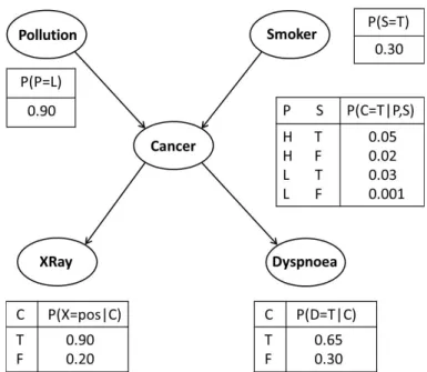
Figure 2.1 gives a simple example of Bayesian network that portrays the probabilistic re-lationships among binary variables Polution (P), Smoker (S), Cancer (C), XRay (X) and Dyspnoea (D). The table associated with each variable is called Conditional Probability Table (CPT), encoding the conditional probability distribution of the variable given its parents. The joint probability distribution of the five variables can be written as
p(P, S, C, X, D) =p(P)P(S)p(C|P, S)p(X|C)p(D|C). (2.2)
As the conditional probability distribution can be calculated from the joint probability, a Bayesian network consisting of a class variable and feature variables is readily applicable to the classification task. Take the lung cancer network as an example, if we chooseCancer (C) as the class variable (value unobserved), we can compute the probability of C =T given any observed value set (p, s, x, d) as
p(C=T|p, s, x, d) = p(C=T, p, s, x, d)
p(C=T, p, s, x, d) +p(C =F, p, s, x, d),
where p(C = T, p, s, x, d) and p(C = F, p, s, x, d) can be computed efficiently using Eq.(2.2). Similarly, we can compute p(C = F|p, s, x, d). Then we decide the value of C by comparing
p(C = F|p, s, x, d) and p(C = T|p, s, x, d). Note that this is a binary classification, easily generalized to multi-class classification by comparing the conditional probabilities of all values of the class variable.
The Bayesian network structure and its associated CPDs can be specified with the help of domain knowledge, e.g., the lung cancer network. However, in most cases, the network structures and CPDs are unknown due to the lack of domain knowledge. In these cases, a Bayesian network classifier can be learned from training data. The learning process contains structural learning and conditional probability distribution estimation. In structural learning,
Figure 2.1: A simple example of Bayesian network: Lung cancer network.
a scoring metric is employed to evaluate the fitness of a structure in relation to the training data. Then, a search method is applied to find a good model [63] among possible structures. Since the number of possible structures is super-exponential with respect to the number of variables, finding the optimal structure is NP-hard [15]. Thus, some heuristic or approximate methods, such as greedy search, are used. However, the model structures selected in this way are often suboptimal. After the structure is constructed, the CPDs can be efficiently estimated using well-developed statistical methods such as Maximum Likelihood Estimation (MLE) or Bayesian Estimation [33].
2.2.2 Bayesian Model Averaging of Bayesian Network Classifiers
Regardless of types of the search methods used, these search methods suffer from the lack of distinguishability of scoring metrics when the training data is sparse, i.e., the size of the dataset is small relative to the number of variables. In this case, there can be many distinct Bayesian networks fitting the training data equally well. Thus, using a single Bayesian network potentially leads to poor predictions on future data.
A promising solution to alleviate this problem is to employ BMA, which provides a princi-pled approach to the model-uncertainty problem by integrating all possible models weighted by their respective posterior probabilities. Formally, given a training datasetDand a future data pointx (a realization of the variable setX), we compute the posterior probability of observing
x as
p(x|D) =X G
p(x|G, D)p(G|D), (2.3)
where p(G|D) specifies the posterior probability of a Bayesian network G given the training data D. p(G|D) can be computed from commonly used scores such as BDe score [25]. Then,
p(x|G, D) can be computed by Eq. (2.2), as the network structureGis fixed in the conditional setup.
Since computing Eq.(2.3) requires enumerating all possible networks, which is super-exponential with respect to the number of variables, it is not of practical use. One solution is to approximate this exhaustive enumeration by using a selected set of model structures inG, i.e.,
p(x|D)≈ P G∈Gp(x|G, D)p(G|D) P G∈Gp(G|D) .
Dash and Cooper [16] described an efficient solution to BMA for prediction over the set of Bayesian network structures consistent with a partial ordering and with bounded in-degree. However, this approach is of limited applicability as it performs model averaging over only a restricted class of BNs consistent with a particular partial ordering. Thus, only a small portion of probability density can be accounted for. Tian et al. [58] proposed to find the
k-best Bayesian network structures and use them to approximately compute p(h|D), i.e., the posterior probability of any hyperthesish. They implemented this idea to address the problem of structure discovery in BNs, i.e., computingp(f|D), the posterior probability of the presence of any structural featuref. (e.g., an edge, in BN structures). They showed that the approximation achieved reasonable accuracy and outperformed the classical sampling methods such as MCMC [18] for structure discovery in BNs. In this study, we employ this idea to address the problem of model averaging for prediction (classification). We select the k-best Bayesian networks
G1, ..., Gk, and use them to approximately computep(x|D) as shown in Eq.(2.4),
p(x|D)≈ Pk i=1p(x|Gi, D)p(Gi|D) Pk i=1p(Gi|D) . (2.4)
Once p(x|D) is computed, we could build a classifier to predict the value of any class variable as shown in Section2.2.1. Whenk= 1, we select the best Bayesian network and use this single network to build a classifier. Thus, it is a special case of BMA.
2.2.3 Finding the k-best Bayesian Network Structures
In previous sections, we mentioned that the optimal model selection is an NP-hard problem, as the number of possible model structures is super-exponential with respect to the number of variables. Thus, in existing applications of Bayesian network classifiers, heuristic or approxi-mate methods are employed to find the models which are usually suboptimal. Silander et al. proposed a dynamic programming (DP) algorithm which is capable of finding the globally op-timal Bayesian network inO(n2n) time [53]. Tianet al. [58] extended the DP algorithm to find the top k Bayesian network structures. They demonstrated the applicability of the algorithm on networks with up to 20 variables. One nice feature of their method is that the estimation accuracy can be improved monotonically by spending more time to compute for larger k.
In this study, we employ this algorithm to select thek-best Bayesian network structures. We then estimate the CPDs using Bayesian Estimation for each of the k-best network structures that result inkdiscrete Bayesian network classifiers. Afterwards, we build our BNMA classifier by averaging the prediction results over the k-best Bayesian network classifiers.
In detail, we use 12 observed feature variables from the KDD Cup 99 dataset and 1 unob-served variable representing intrusion or not intrusion. We get the k-best Bayesian Network structures by running the software tool called KBest [58] which is used to compute the posterior probabilities of features by Bayesian model averaging over the k-best Bayesian networks. Inside of this tool package, it computes the local scores for all the families of each variable. With a selected k value, the software tool of KBest takes a file of data records as input and outputs thek best network structures and lists the estimated posterior probabilisties for each of the k
2.3 Description of NSL-KDD Dataset
In previous IDS research, KDD Cup 99 dataset has been widely used to help build and evaluate these systems [4] [63] [3] [17]. This database contains a standard set of data to be audited, which includes a wide variety of intrusions simulated in a military network environ-ment. However, KDD Cup 99 has two major issues that highly affect the assessment of the performance of evaluated systems [57]. The first deficiency in KDD Cup 99 dataset is the huge number of redundant records in the training dataset. This deficiency will cause learning algo-rithms to be biased towards more frequent records. The second deficiency is that the existence of repeated records in the test set will cause the evaluation results to be biased towards favoring the methods with better detection rates on frequent records.
In our experiment, we use the NSL-KDD [57] dataset, a new version of KDD Cup 99 dataset consisting of selected records of the complete KDD Cup 99 dataset with redundant and repeated records removed. As can be seen from the literature [57], the original KDD Cup 99 dataset is skewed and unproportionately distributed, training and testing directly on the KDD Cup 99 dataset can result in relatively high accuracy rate for different methods, making it difficult to effectively compare different classifiers. Using this NSL-KDD dataset for evaluation is more objective and judicial as it does not suffer from either of the two problems mentioned above. The NSL-KDD dataset contains a training set with 125,973 records and a testing set with 22,544 records. Each of the datasets contain 41 attributes describing different features of the connection and a class label assigned to each either as attack or as normal.
2.4 Construction and Evaluation of BNMA Classifier
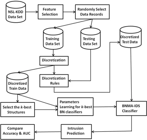
In this section, we introduce how we construct and evaluate the BNMA classifier. Figure2.2 illustrates the process from data processing to classifier training and evaluation. The whole process is elaborated in the following steps:
1. Download NSL-KDD dataset and select a subset out of a total 41 features as the variables for classifier building.
2. Randomly sample partial datasets of varying sizes from the overall NSL-KDD training dataset as the training sets. The whole NSL-KDD testing dataset is then used as the testing set.
3. Perform data discretization on the continuous features in training and testing datasets using the information-preserving discretization method.
4. Find the k-best Bayesian network structures using the training dataset, and estimate the CPDs for each networks using Bayesian Estimation. This results in k independent Bayesian network classifiers.
5. Combine the kBayesian network classifiers into a Bayesian classifier using BMA.
6. Apply the Bayesian classifier to the testing dataset, calculate the accuracy and Area Under ROC (AUC).
7. Conduct four groups of experiments by repeating steps 2-6 using different training sets. The results for each classifier and each configuration of different size are then averaged over those four groups of experiments.
In the upcoming subsections, we give details on the process of feature selection, data dis-cretization, and classifier training and evaluation.
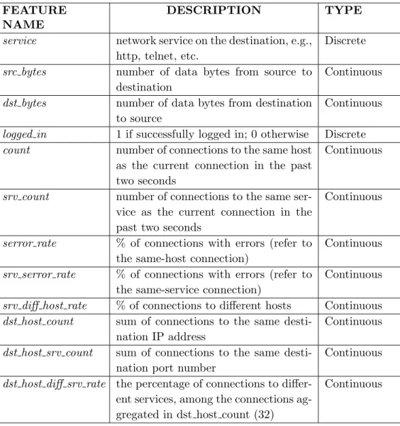
2.4.1 Feature Selection
Feature selection is an indispensable pre-processing step when training a huge dataset with many features. Extraneous features not only add burden to the computation but also confound the detection process. The NSL-KDD dataset contains 41 features, some of which may be redundant and contribute less than the others to the detection process. Feature selection and feature deduction have been a very popular topic in intrusion detection field for identifying important input features to build computationally efficient and effective IDS. Singh & Silakari [54] proposed an ensemble approach for feature selection of the Cyber Attack dataset. Chebrolu et al. [12], Kayaciket al. [30] and Olusolaet al. [46] specifically analyzed the feature relevance on the KDD Cup 99 dataset. In [12], Markov blanket model was used to select the feature
Figure 2.2: Flowchart illusrating the training and evaluation of BNMA classifier
set and it was shown that a selected set of 12 features can achieve better predictive accuracy than when the whole set of 41 features is used. Our main focus in this paper is to compare the methods based on the same datasets with the same feature set, rather than to study the KDD data. And we are also particularly interested in studying their performance using a carefully selected representative subset rather than the full features. Therefore, in our experiments we used the 12 features suggested in [12]. Those features are described in the following Table2.1.
2.4.2 Data Discretization
As shown in Table 2.1, some of the selected features take continuous values. However, current implementation of Bayesian network classifiers can only handle discrete values. Thus, continuous features need to be discretized before being used to build a classifier. On the other hand, discretization can often make continuous features easier to understand and interpret, and produce faster learning models. Many learning models have been shown to perform better by
Table 2.1: List of Selected Features
FEATURE NAME
DESCRIPTION TYPE
service network service on the destination, e.g.,
http, telnet, etc.
Discrete
src bytes number of data bytes from source to
destination
Continuous
dst bytes number of data bytes from destination
to source
Continuous
logged in 1 if successfully logged in; 0 otherwise Discrete
count number of connections to the same host
as the current connection in the past two seconds
Continuous
srv count number of connections to the same
ser-vice as the current connection in the past two seconds
Continuous
serror rate % of connections with errors (refer to
the same-host connection)
Continuous
srv serror rate % of connections with errors (refer to
the same-service connection)
Continuous
srv diff host rate % of connections to different hosts Continuous
dst host count sum of connections to the same
desti-nation IP address
Continuous
dst host srv count sum of connections to the same
desti-nation port number
Continuous dst host diff srv rate the percentage of connections to
differ-ent services, among the connections ag-gregated in dst host count (32)
discretizing continuous features [36]. Based on our knowledge, there are two types of commonly used discretization methods in many of the IDS [37] [46] [63], that is, the unsupervised dis-cretization algorithms, e.g., equal intervals, equal frequencies, and the supervised disdis-cretization algorithms, e.g., maximum entropy discretization,χ2 discretization, CAIM, etc. In our exper-iment, we adopted a discretization algorithm named CACC [59], which was a a static, global, incremental, supervised and top-down discretization algorithm. This information-theoretic al-gorithm extended the idea of contingency coefficient, combined with the greedy method, and was empirically shown to be promising in terms of accuracy, execution time, etc. Data dis-cretized using such discretization scheme have much less information loss, thus better represent the distribution of original data compared to the ones discretized using other unsupervised discretization methods.
2.4.3 Classifier Training and Evaluation
One purpose of this study is to evaluate the performance of various classifiers with respect to varying sizes of the training dataset. Thus, we prepare several training datasets containing 500, 1000, 2000, 5000, 10000, 20000, 30000, 40000 records, respectively. We train and build a Bayesian classifier from each of the training sets by BMA over thek-best Bayesian network classifiers as described in Section2.2. For each training dataset, we build the Bayesian classifier by settingk to various values. We then evaluate the performance of the classifier with respect to these differentkvalues. Whenk= 1, the classifier is equivalent to a single Bayesian network classifier. The largerkis, the more models are employed for model averaging, which potentially leads to better predictive power.
We evaluate all classifiers on the same testing dataset. We compute the accuracy as the percentage of correctly classified records. Note that this is a binary classification problem, i.e. an attack or normal. A record is classified as an attack if the conditional probability of being an attack given the observation of other features is greater than 0.5; it is classified as normal otherwise. In addition to accuracy, we compute AUC as the area under the Receiver Operating Characteristic (ROC) curve, which is an estimate of the probability that a classifier will rank a randomly chosen positive instance higher than a randomly chosen negative instance. Since
AUC does not depend on the classification threshold used, it is widely recognized as a better measure than accuracy, which is based upon a single classification threshold.
For comparison, we also build Naive Bayes classifiers and Bayesian network classifiers, which are selected by using the greedy hill-climbing search method. The training and testing processes of this two classifiers are executed in the open source software of Weka which is a collection of machine learning algorithms for solving real-world data mining problems. Weka is written in Java and runs on almost any platform. The algorithms can either be applied directly to a dataset or called from user’s own Java code. When we use Weka to train and test the Naive Bayes classifiers and Bayesian network classifiers, we just need to pass a file of training records and a file of testing records separately to it and Weka gives detection accuracy and AUC result based on the input training and testing dataset. We implemented our algorithm of BNMA classifier and added it to Weka as a new algorithm. With the training dataset, testing dataset andk-best network structures given by KBest software as input, our implemented classifier can output the detection accuracy and AUC of using BNMA over the input dataset.
As described before, we repeated the experiment four times on different training and testing data sets with each training size andkvalue. We reported the average accuracy and AUC over the four trainings for each training size andkvalue. Considering the records of training dataset and testing dataset are selected randomly from NSL-KDD dataset, the averaged result over four experiments is more reliable and objective than the result based on one experiment.
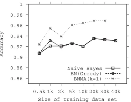
2.5 Experimental Results
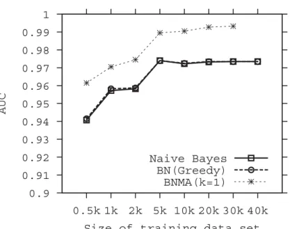
Figure2.3compares the detection accuracy of Naive Bayes (NB), Bayes Network built using greedy search (BN-Greedy) and the BNMA (k= 1) by size of the training dataset. First, we observe that the accuracy is approximately a non-decreasing function of training sample size. This is understandable since a larger training sample usually produces a classifier with better predictive power. The accuracies of NB and BN-Greedy are comparable to each other, while the BNMA classifier built using the best Bayesian network (k= 1) is significantly better than the two classifiers. Further, the BNMA (k = 1) trained classifiers using a small training set (2000) even outperforms the NB and BN-Greedy classifiers trained using a very large training
set (40000). The improvement is also significant when AUCs are compared (see Figure 2.4). This indicates that the BNMA classifier can achieve reasonably good predictive power even when a small training dataset is used.
0.86 0.88 0.9 0.92 0.94 0.96 0.98 1 0.5k 1k 2k 5k 10k 20k 30k 40k Accuracy
Size of training data set Naive Bayes
BN(Greedy) BNMA(k=1)
Figure 2.3: Comparison of detection accuracy by size of training set
In another set of experiments, we evaluate the BNMA classifier with respect to various k
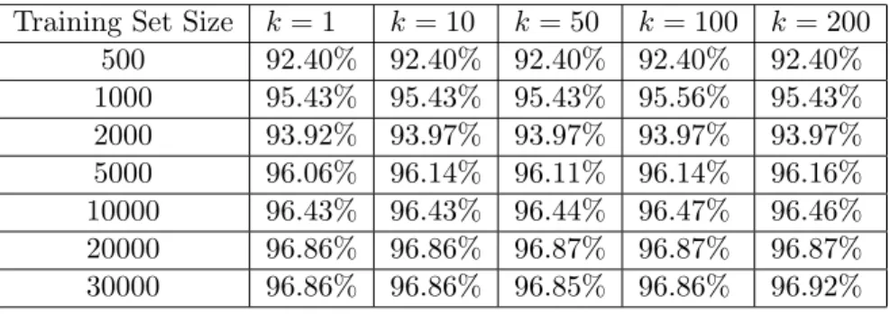
values. Table2.2 compares the detection accuracy by k value and training set size. Table 2.3 compares the AUC by k value and training set size. It is shown that with the increase of k, both accuracy and AUC increase. AUC has a more obvious increase than accuracy. However, this improvement is not as significant as that in comparing BNMA (k= 1) with NB and BN-Greedy. The most significant improvement is in Table2.3, for sample size 500, where the AUC jumps from 0.9615 for k = 1 to 0.9733 for k = 200. With the increase of sample size, the improvement decreases. This demonstrates that the BNMA is particularly effective on small sample sizes.
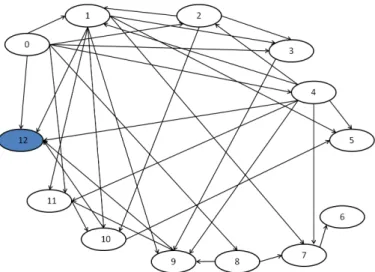
To investigate why the predictive power does not change very much with respect to the variation of the k value, we examine the structures of the top 10 networks produced using a training set with size 10000. Figure2.5illustrates the consensus structure for the 10 structures.
Table 2.2: Accuracy Comparison byk Value and Size of Training set
Training Set Size k= 1 k= 10 k= 50 k= 100 k= 200
500 92.40% 92.40% 92.40% 92.40% 92.40% 1000 95.43% 95.43% 95.43% 95.56% 95.43% 2000 93.92% 93.97% 93.97% 93.97% 93.97% 5000 96.06% 96.14% 96.11% 96.14% 96.16% 10000 96.43% 96.43% 96.44% 96.47% 96.46% 20000 96.86% 96.86% 96.87% 96.87% 96.87% 30000 96.86% 96.86% 96.85% 96.86% 96.92%
Table 2.3: AUC Comparison by kand Size of Training set
Training Set Size k= 1 k= 10 k= 50 k= 100 k= 200
500 0.9615 0.9706 0.9733 0.9733 0.9733 1000 0.9705 0.9718 0.9728 0.9728 0.9730 2000 0.9738 0.9738 0.9740 0.9744 0.9745 5000 0.9895 0.9898 0.9898 0.9900 0.9900 10000 0.9905 0.9905 0.9905 0.9908 0.9908 20000 0.9928 0.9928 0.9928 0.9928 0.9930 30000 0.9933 0.9933 0.9933 0.9933 0.9933
0.9 0.91 0.92 0.93 0.94 0.95 0.96 0.97 0.98 0.99 1 0.5k 1k 2k 5k 10k 20k 30k 40k AUC
Size of training data set Naive Bayes
BN(Greedy) BNMA(k=1)
Figure 2.4: Comparison of AUC by size of training set
It is surprising that all 10 structures share the same skeleton with minor differences in the direction of the edges. This indicates that the top structures represent similar distribution, and thus make similar predictions for new data points. We can speculate that the top 200 structures may have very similar structure. For comparison, we also depict the Bayesian network structure learned using greedy hill climbing search method in Figure 2.6. It is easily observed that this structure is significantly sparser (fewer edges) than the consensus structure in Figure2.5. This explains why the structure selected with heuristic method is suboptimal, because it fails to identify many important dependencies among the feature nodes which can be captured by our method of using BNMA classifier. It also explains why the best Bayesian network (k= 1) has significantly better predictive power than the BN-Greedy classifier.
2.6 Conclusion and Future Work
In this study we proposed a Bayesian classifier using BMA of k-best Bayesian network classifiers, called BNMA classifier, for intrusion detection. Previous IDS using Bayesian network classifier has two problems. First, the Bayesian network structure is selected using heuristic
Figure 2.5: A consensus network built from the top 10 networks trained on sample size 10000. The correspondences between the nodes and the features are : 0-service; 1-src bytes; 2-dst bytes; 3-logged in; 4-count; 5-srv count; 6-serror rate; 7-srv serror rate; 8-srv diff host rate; 9-dst host count; 10-dst host 8-srv count; 11-dst host diff 8-srv rate; 12-class (intrusion or not intrusion). Note that the class variable is shadowed. Directed edges existing in all 10 structures are depicted as solid arrows. The set of edges that exist in all structures but with various directions are depicted as solid lines.
Figure 2.6: The Bayesian network trained on sample size 10000 using greedy hill climbing search method. The correspondences between the nodes and the features are the same as those in Figure 2.5.
methods, which usually return suboptimal models. Second, previous classifiers are trained and evaluated using a very large training dataset, which is usually hard to collect within a short time period. In this study, we used a DP algorithm to find the globally k-best structures and used them to build a Bayesian classifier by BMA. We showed that the BNMA classifier has significantly better predictive power than Naive Bayes and the Bayesian network classifier built using heuristic method. Even the classifier trained using a very small dataset outperforms the other two classifiers trained using a very large dataset. We then conclude that our BNMA classifier is particularly effective in detecting intrusions when only a few training records are available. This is very valuable since prompt detection of intrusion is of significant importance in such an era of rapidly growing Internet activities.
We also show that with the increase of k, i.e., more Bayesian network classifiers are used for model averaging, the better predictive power it can achieve. However, this improvement is not that significant, since the top structures actually share a very similar structure. This means the problem size (12 feature variables) is still not that large compared to the sample sizes examined. One question that users may ask is, what is the k value we should use? The answer is the larger, the better. However, it takes more time to train and integrate over larger number of classifiers. In this study, we consider 12 feature variables and k = 100 is already enough. Thek value that should be selected depends on the problem size, i.e., the number of feature variables used to build the model. Thus, our future work is to select a larger set of feature variables for model building. Since Bayesian network is able to inherently do feature selection through its conditional dependency assertions, using a larger set of features should not significantly impact the performance. However, with a larger set of feature variables, it may need larger k, i.e., integrating over more models to achieve reasonably good predictive power.
Another area for future work is based on the observation that intrusions happen in dynamic environments, thus they themselves could be time-series data. An et al. [5] proposed to use dynamic Bayesian networks to model the temporal environment. However, the problems faced by the static Bayesian network classifier persist in dynamic Bayesian networks. Thus, it is a challenge to perform model averaging in the temporal environment setup.
In summary, since it uses less data while still achieving comparable or better predictive power, our BNMA classifier can save a huge amount of time on collecting training data records so that it can catch the intrusion more promptly and more accurately to avoid loss due to intrusion.
CHAPTER 3. SITUATIONAL DATA FOR INTRUSION DETECTION SYSTEM
Abstract
Intrusion detection is a research topic of great importance, especially for web-based appli-cations, whose broad usage at the same time makes themselves attractive targets for malicious attackers. Meanwhile, applications of many emerging new web techniques (e.g., Web 2.0, HTML5, and cloud computing, etc.) add more challenges to intrusion detection. One signifi-cant issue of building Intrusion Detection System (IDS) is to find an efficient and informative training data set. In this paper, we proposed a Situational Data Model which is represented by a sequence of observed situations. Our main contributions can be summarized as follows. First, we designed Situational Data Model that has better data structure and is more informative. Each data record is a sequence of situations collected in chronological order. At each time point, the situation contains a series of information including the context and action for the possible intrusion, and potential intruder’s desire. Different from action sequences data and state sequence data, Situational Data makes the training process be able to be performed over the sequence of punctuated desires which can be inferred from the sequence of actions and con-texts. The valuable footprints of transition from one situation to another are well captured by this data collection mechanism. Second, we collected the training data from a real web applica-tion system Cooperative Research Environment(CoRE) which is developed for research use by Software Engineer Research Group in the Department of Computer Science at ISU. Our train-ing data set provides valuable evaluation reference for dynamically intrusion detection system such as Hidden Markov Model based IDS. Third, we compared our Situational Data against the data comprised of action sequences data by employing the Hidden Markov Model, and the
result approves that Situational Data with desires can bring better classification accuracy and ROC curve.
Key Words: Intrusion detection system, Situ, Hidden Markov Model, detection accuracy, ROC
3.1 Introduction
In this chapter we introduce the Situational Data Model for building dynamic intrusion detection system. This Situational Data Model is based on the Situ framework introduced by Chang et al. [11], and is defined by situational data consisting of environmental context information, activities, and inferred desires.
Traditionally, there are two categories of intrusion detection systems, i.e., either misuse-based or anomaly-misuse-based. A misused-misuse-based intrusion detection system includes a number of attack descriptions or signatures trained from abnormal data. It gives intrusion alert whenever a stream of audited data matches with an attack model. On the other hand, an anomaly-based intrusion detection system relies on models trained from the normal data. Deviations of audited data from established models are interpreted as potential attacks [42]. Training data are usually collected from network, operating systems, or application log files. Various data sets are used in building all different kinds of intrusion detection systems. Through training on historical data, a model explaining the relationship between intrusion and selected features can be built. The established model is then used to predict outcomes for future audited data. For instance, Kruegel and Toth [39] created a decision tree to detect malicious events, based on a set of signatures of data constraints. Altwaijry [2] developed a na¨ıve Bayesian classifier to identify possible intrusions. To evaluate an intrusion detection system, the public KDD Cup 1999 dataset [31] has been widely used by the researchers for experiments in the literature [14,63]. This dataset contains 41 feature variables and up to 4 million staggering records. Also, the feature variables of the KDD Cup 1999 dataset include network traffic information such as src bytes (number of data bytes from source to destination), dst bytes (number of data bytes from destination to source), and protocol type (type of protocol), etc. The classical approaches
typically first train a model based on selective features using a certain amount of data, then predict a future data record to be intrusive or normal based on the trained model. However, one common limitation of all those training data is that they only have static network traffic data, and do not take into account the dynamic nature of many features that may change over time. This may be partly due to that their feature values were collected statically without any time stamp. Therefore, they treat all different features being time-independent and ignore potential temporal relationships between the same features at different time points. In fact, the dynamic transitions of features’ value in chronical order often carry important information, and can be very valuable for detecting the intrusions. For example, under statistic data structure, a potential anomalous behavior that repeatedly have massive amount of data bytes flowing from source to a destination at different time periods may not be distinguishable from a normal behavior with similar situation at a single time point. In this case, it may be very challenging for us to catch the intrusion if we just model the static context information in spite of the features being time dependent.
Dynamic features have been shown to be more efficient than static features. In fact, some researchers have been using sequential data for training intrusion detection models. For in-stance, Ariu et al. [7] designed the intrusion detection system HMMPayl, which uses the Hid-den Markov Model to analyze the HTTP payload, to detect attacks against Web applications. Those authors expressed the payload as a sequence of bytes and showed that the HMMPayl is very effective against attacks like Cross Site Scripting [22] and SQL-Injection [35], whose payload would not be significantly different from that of normal traffics. On the other hand, the detection system proposed by Chen et al. [13] analyzed multiple logs from cloud to extract the intention of the actions recorded in the logs. In their work, the Hidden Markov Model was adopted to model the sequence of actions performed by hackers. Such stealthy events in a long time frame is significantly more useful for training the state-aware model. Besides, in [27], sequences of systems calls were used to build the classification schema. However, all those sequential features and data used in their IDS training do not have the human internal mental states (desires) involved. Human desires which could be driven from other features are more correlated to or more representative of human’s intention than those features. In this thesis, we
propose a situational data model with actions, contexts of target web application system and desires of human. We collect and parse the data following the Situ framework [11]. That is, we represent each data record as a sequence of situations, of which each contains three components – desire, action, and context. We then compare Situational Data Set with action-only sequences dataset using the Hidden Markov Model. Our experiment result shows that situational dataset is more effective by having the training process guided by human desires.
The rest of this chapter is organized as follows: Section 3.2 introduces the related work Hidden Markov Model and Situ Framework. Section3.3 describes the Situational Data Model and the process of Situational dataset collection. Section 3.4gives our experiment design and results. Finally, we conclude in Section3.5with a summary of the current work and a discussion of potential future work.
3.2 Related Work
3.2.1 Hidden Markov Model
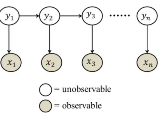
A hidden markov model (HMM) is a statistical model representing probability distributions over a sequence of observations, say {x1, . . . , xT}, accompanied by hidden states {y1, . . . , yT} [21]. As a simple dynamic Bayesian network model, a HMM can be illustrated by Figure3.1, and there are two defining properties: hidden, in the sense that all observations{xt, t= 1, . . . , T}are assumed to be generate by some process whose states{y1, . . . , yT}are hidden; Markov property, in the sense that the distribution of those hidden states have markov property, i.e., at any time pointt, the distribution ofytgiven all its historyy1, . . . , yt−1is equivalent to that ofytgivenyt−1
only. In addition, the conditional distribution of any the observations xt given all other nodes of the graph is the same as its conditional distribution given its immediate parentyt. Bringing those markov properties together, the joint distribution of (X, Y) = (x1, . . . , xt, y1, . . . , yt) can be written as p(X, Y) = T Y t=1 p(xt|yt)p(yt|yt−1),
Figure 3.1: Hidden Markov Model
HMMs have been widely used in the literature for researches in different disciplines, e.g., economics, computer science, etc. HMM is also very often used in intrusion detection [7,13,27]. In applications, typically a parametric model is assumed for the joint distribution of p(X, Y) such that p(X, Y) = p(X, Y;θ), and the goal of learning task is to obtain an estimator for
θ based on observed outcomes X = (x1, . . . , xT). Intuitively, because Y = (y1, . . . , yT) are hidden, i.e., unobserved, θ may be estimated by the marginal distribution of X, i.e.,
p(X;θ) = P
y1,...,yTp(X, Y;θ). However, obtaining the marginal distribution may be
chal-lenging in practice and computation can be intensive using this brute-force approach. Never-theless, in the literature efficient computational algorithms are available, e.g., E-M algorithm based Baum-Welch method [45], among others. In our discussion here, we use HMM model as a candidate method for comparing the effectiveness of Situational Dataset with another dataset in training Intrusion Detection System and classifying intruders and normal users. Details re-garding how HMM is applied in our setting and how HMM is to be combined with the Situ framwork will be introduced in the upcoming discussions and section.
Figure 3.2: Situ Framework
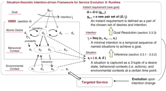
3.2.2 Situ Framework
The data records used for training and prediction is modeled following the Situ Framework. Situ Framework [11] originally provides a situation-theoretic approach to human-intention-drive service evolution in context-aware service environments. The situation defined in this framework is rich in semantics and useful for capturing human thinking and behavioral patterns, which, in turn, help developers to construct the intention specification. Figure 3.2 from [11] shows the situation-theoretic intention-driven framework for service evolution at runtime.
In Situ framework [11], a human intention is defined as temporal sequence of situations to achieve a goal, which is described asI = seq(S1, S2, . . . , Sk) whereS1, . . . , Sk are goal-directed situations for the goal g. A situation at time t is expressed as situation (t). It is a triple {d, A, E} in which d is the predicted users desire, A is a set of the users actions to achieve a goal which d corresponds to, and E is a set of environment context values with respect to a subset of the context variables at timet. As shown in Figure3.2, an intention plays a proactive role in interpreting human actions, which are the key component connecting desires and specific contexts. The contexts are derived from sensing the entire environment surrounded by a user
being observed in a service system. This type of contexts such as time, location and so on is helpful in understanding the triggers and effects of human’s actions. The actions are derived from human behaviors which interact with contexts bidirectionally. Situ is a higher level formal mechanism to understand human intention change by the situations.
3.3 Situational Data for Intrusion Detection
3.3.1 Definition of Situational Data Model for Intrusion Detection
In previous intrusion detection researches, the KDD Cup 1999 dataset has been widely used to build and evaluate the Intrusion Detection System [14,63]. The KDD Cup 1999 dataset [57] include many relevant features such as connection, traffic, and content, etc. However, all of those features are static, in that no time stamps are associated with those features that could potentially change over time. Therefore, a potential layer of correlation or connection between those features is missing. In other words, features collected at two different time points, sayt1
and t2, are treated as two entirely independent records regardless of their time stamp. We call
those type of data as static data. In a static data model, the over-time trajectory of features are not collected thus cannot be used in training or utilized to predict audited data in the future.
When only static data are used for training, it is very difficult to detect malicious attacks that have similar network traffic features as normal behaviours, e.g., SQL injections. This naturally motivates making use of training data that can capture not just statistic features but also dynamic characteristics. For instance, sequential data that are collected with time stamps would help counter this challenge. In fact, sequential data have already been frequently used in the literature. For example, Ariu et al. [7] defined each data record as a sequence of payload bytes length collected at different time points. While this data model captures the payload bytes length in a sequential manner for intrusion detection, it is, however, not effective for detecting attacks that do not cause significant payload changes over different time points. For illustration, we can think of a simple example where a brute-force type attack is considered. Specifically, suppose an attacker repeatedly tries to log-in by guessing passwords without being
successful. In this case, the payload bytes length at each of those attempts will not differ much from each other, thus the system will probably fail to detect this attack.
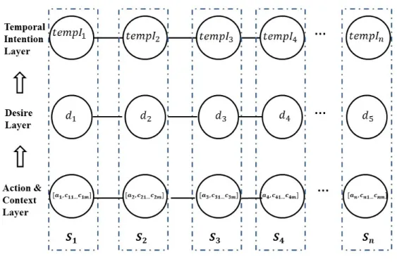
Given reasons above, we believe that it can be more effective for intrusion detection if we consider not only the change of general context, e.g., payload byte length, but also other factors such as sequences of users’ behaviors and thinking patterns. Following this thought, we build our Situational Data model based on the Situ framework [11]. According to the correlations of intention, desires, context, and actions described in Situ, we design our Situational Data model with three layers as shown in Figure 3.3. Specifically, lett1, . . . , tnbe data collection time points in natural chronical order. The first layer represents action and context sequences, denoted by [A1, C1], . . . ,[An, Cn]. Then the second layer captures the desire sequence, d1, . . . , dn. The third layer gives the temporal intention sequence tempI1, . . . , tempIn. A user’s footprint left in the system is expressed as a sequence of situations, say, S1, . . . , Sn. Each situation St at time pointt consists of [At, Ct], dt andtempIt, where [At, Ct] is the set of actions and context observed at timet,dt is the user’s desire on the system at timet, andtempIt is a quantitative value indicating the degree of the segmental attacking intention for the desire at time t. A user’s intention is then composed of a sequence of situations.
For intrusion detection purposes, one of the key components of the Situational Data Model is the desire layer which plays a central role as a bridge in the process of inferences in classification. It helps find hidden relationships among those trivial context and behavior information, then help correlate them with users’ temporal intentions. It guides the predictive model with clearer direction on classifying intruders and normal users. When attackers have malicious intentions, they tend to plan and execute the attack step by step. Using a metaphor to illustrate the relationship among actions, environment context, human desires, and intention in a system, we can think of the preparations a smart robbery might do after he decides to rob. The intention of rob drives him to have some temporal desires such as avoiding to be recognized, avoiding to be recorded by camera, confirming no polices around, and so on. Those temporal desires then drive him to have some actions and context information like wearing sun glasses, wearing a mask, observing possible cameras, and so on, leading to a abnormal sequences of actions and environment context. The same for attacking computer systems, a user with malicious intention
Figure 3.3: Situational Data Model
must have attacking-driven desires at some of the time points in the situation sequence. Those desires will then drive the attackers to learn vulnerabilities and information about the target system before he is able to intrude eventually. During the process of learning vulnerabilities and trying attack, the attackers would have abnormal behaviors, which make the environment context different from that of normal users’.
To use this Situational Data Model, we need to train two prediction models. The first model is a desire model for predicting the desire sequence based on action and context sequences. The other model is an intention model for predicting temporal intention by desire sequences. When IDS is used to predict and detect intrusion, firstly we treat action and context sequences, i.e., [A, C], as observed data and desire sequences as hidden state data to be predicted. Secondly, the predicted desire sequences from the desire model will be used as input of the intention model for predicting the temporal intention sequences. Finally, the trained IDS can classify an intention to be normal or malicious according to the values of the temporal intention sequence
3.3.2 SQL Injection
In this subsection, we briefly describe one of the intrusion techniques used by assumed intruders in our data collection platform, i.e., CoRE. We explain how SQL injection happen since it is most frequently used by our assumed intruders.
In web based applications, when normal users submit their input information on the client side, the input value will be combined by a SQL statement written by programmers. For instance, suppose a normal user enters marcus as the username andsecret as the password in the log-in page from the client side. The web-based application will interpret it in the way that is described by the following SQL statement:
SELECT * FROM users WHERE username = ’marcus’ and password = ’secret’
Subsequently, this statement will search the user database and retrieve all relevant information that matches the user namemarcus and passwordsecret.
When a malicious user intrudes the system using the SQL injection technique, the main idea is to bypass the above user name and password check by injecting some input values that can turn the above concatenated SQL statement into an always-true statement regardless of the actual user name and password provided. This is because the website log-in program is written in such a way that it interprets log-in information by combining the phrases from “username” and “password” fields in the SQL statement, in the same way as the example shown in the previous paragraph. As a result, because the SQL statement is true, the log-in system will then grant access to the intruder. For example, suppose an attacker knows the database administrator’s user name,admin. Then the attacker may capitalize on this and use this information in the log-in page by entering the username admin’–. This input will then generate a SQL statement as follows:
SELECT * FROM users WHERE username = ’admin’- -’ and password = ’anything’
Note the sign 0 − −0 is an annotation mark in SQL syntax, thus all the following statement