(will be inserted by the editor)
Predicting Interval Time for Reciprocal Link
Creation using Survival Analysis
Vachik S. Dave · Mohammad Al Hasan ·
Baichuan Zhang · Chandan K. Reddy
Received: date / Accepted: date
Abstract The majority of directed social networks, such as, Twitter, Flickr, and Google+ exhibit reciprocal altruism, a social psychology phenomenon, which drives a vertex to create a reciprocal link with another vertex which has created a directed link towards the former. In existing works, scientists have al-ready predicted the possibility of the creation of reciprocal link—a task known as “reciprocal link prediction”. However, an equally important problem is de-termining the interval time between the creation of the first link (also called parasocial link) and its corresponding reciprocal link. No existing works have considered solving this problem, which is the focus of this paper. Predicting the reciprocal link interval time is a challenging problem for two reasons: First, there is a lack of effective features, since well-known link prediction features are designed for undirected networks and for the binary classification task, hence they do not work well for the interval time prediction; Second, the pres-ence of ever-waiting links (i.e., parasocial links for which a reciprocal link is not formed within the observation period) makes the traditional supervised regression methods unsuitable for such data. In this paper, we propose a solu-tion for the reciprocal link interval time predicsolu-tion task. We map this problem to a survival analysis task and show through extensive experiments on
real-V. S. Dave, M. Al Hasan
Department of Computer & Information Science IUPUI, Indianapolis, USA
[email protected], [email protected] Baichuan Zhang
C. K. Reddy
Department of Computer Science Virginia Tech, Arlington, USA [email protected]
___________________________________________________________________ This is the author's manuscript of the article published in final edited form as:
Dave, V. S., Hasan, M. A., Zhang, B., & Reddy, C. K. (2018). Predicting interval time for reciprocal link creation using survival analysis. Social Network Analysis and Mining, 8(1), 16. https://doi.org/10.1007/s13278-018-0494-1
world datasets that survival analysis methods perform better than traditional regression, neural network based models, and support vector regression (SVR) for solving reciprocal interval time prediction.
Keywords Link Prediction · Directed Network · Reciprocity · Time Prediction· Survival Analysis
1 Introduction
Reciprocity is a phenomenon in social psychology which mandates that peo-ple should repay voluntarily what another person has provided for them. It is different fromaltruism(Anand et al, 2013) in the way that reciprocity follows from others’ initial action, while altruism is a spontaneous action of gift-giving without the hope or expectation of future positive responses. There also ex-ists another social psychology, namedreciprocal altruism, which is a behavior whereby one performs an act of gift-giving with the expectation that the re-ceiving person will act in a similar manner at a later time (Trivers, 1971). People’s day-to-day activities on online social networks are filled with many examples of reciprocal altruism: we follow a friend’s Twitter feed with the hope that he will follow back our feed; we like a friend’s Facebook posts or her Flicker images with the expectation that she will do the same; we endorse our friends for their technical skill in LinkedIn hoping that they will return the favor in a similar manner.
However reciprocity usually is in conflict with another social phenomenon called social stratification, which favors hierarchical arrangement of people in a society based on various factors such as power, wealth, and reputa-tion (Hopcroft et al, 2011). This phenomenon is prevalent in online social networks as well, but in a different manner. Apparently, for such networks, the social hierarchy is reflected in various prestige metrics which rank ver-tices based on their topological bearings, such as pagerank, and in-degree. Given this hierarchical arrangement in an online social network, people who are higher up in the hierarchy are sometimes reluctant to perform a recipro-cal act for an individual who is lower in the hierarchy; they instead defer the reciprocal action to a later time, or sometimes indefinitely.
For reciprocal link creation, understanding the criteria which control the interval time and building learning models which predict the interval time are important. From a research standpoint, such studies help scientists to under-stand the interaction between reciprocity and social stratification phenomena. From the perspective of real-life applications in social network analysis, such prediction models enable better link suggestions, where the interval time is also factored in within the suggestion. Reciprocity, along with the interval time for reciprocal link creation, is particularly important for recommendation in online dating systems (Xia et al, 2015).
The majority of existing works on link prediction assume an undirected net-work (Hasan and Zaki, 2011; Valverde-Rebaza and de Andrade Lopes, 2013), in which the concept of reciprocal edges does not exist. A few works consider
reciprocal link prediction (Hopcroft et al, 2011; Gong and Xu, 2014) in a di-rected network where the prediction is binary, yielding a yes/no answer to the question of whether a reciprocal link will be created within a fixed obser-vation window. Several other works utilize reciprocity as a tool for network compression (Chierichetti et al, 2009) and information propagation in social networks (Zhu et al, 2014). Reciprocal links also influence the degree correla-tions in complex networks, hence they play an important part in modeling the growth of directed social networks (Zlati´c and ˇStefanˇci´c, 2009). However, none of the existing works consider predicting the interval time for the creation of a reciprocal edge.
Extending a model which solves a binary class reciprocal link prediction problem to a model which predicts the interval time of reciprocal links is non-trivial. The major challenge for interval time prediction is that typical link prediction features for an undirected network, such as common neighbors, Jaccard’s similarity, and Adamic-Adar do not have a well-defined counterpart for directed networks, which makes interval prediction a difficult task. Addi-tionally, for generating the training data for building a prediction model, a network is observed for a finite time window, and the absence of a reciprocal link within that time window does not necessarily mean the absence of that re-ciprocal edge, because a rere-ciprocal edge might have formed outside (after) the observation time window. This yields numerous right censored data instances, for which the target variable, i.e., the reciprocal link formation time is not available. Traditional supervised regression models cannot include censored data instances in the training data and hence perform poorly in predicting reciprocal link creation time.
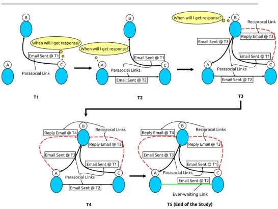
We explain the cases of right-censored data instances in reciprocal interval time prediction task using a toy example shown in Figure 1. In this figure we show a small part of an email communication network consisting of only three vertices representing three persons, A, B, and C. Our observation period of this network has five timestamps,T1 toT5. AtT1,Csends an email toB, thus creating the first of the directed links (such links are called parasocial links). At T2, the parasocial link fromAtoBis created. AtT3, the reciprocal link from BtoCis created; thus the interval time of this edge isT3−T1. AtT3, another parasocial link (B→C) is created. More links are created in subsequent time intervalsT4 andT5. AtT5, we reach the end of our observation period, but the reciprocal link fromC toAis yet to be created. The potential reciprocal linkC→Ais an instance of right-censored data for which we only know that the interval time is higher thanT5−T1; this value, as well, can be infinity in the case that the link is never created. Either way, the exact value of the target variable for this reciprocal edge is unknown. Unfortunately, for any reasonable observation time window, a significantly large number of potential reciprocal links are censored data instances, which is the main challenge for the task of reciprocal link creation time prediction.
In this work, we present a supervised learning model for predicting the interval time for the creation of a reciprocal edge between a pair of vertices in an online social network, given that a parasocial edge already exists between
Fig. 1: An illustration of reciprocal link time predictionRLTP problem.
the vertex-pair. We study real-life networks and validate a collection of topo-logical features that may influence the reciprocal edge creation time. Then, we design the prediction task as a survival analysis problem and propose five censored regression models. Our experimental results show that Cox regres-sion performs better than traditional supervised learning models for reciprocal link prediction. This is an extended version of our previous paper (Dave et al, 2017), which is published in 11th International Conference on Web and Social Media (ICWSM).
2 Related Works
The traditional binary classification task of link prediction has received enor-mous attention over the years since the inception of this problem by Liben-Nowell and Kleinberg in 2003 (Liben-Liben-Nowell and Kleinberg, 2003). Over the years researchers have solved the link prediction problem for a variety of graphs - for example link prediction in homogeneous networks (Hasan et al, 2006; Liaghat et al, 2013; Wang et al, 2017b), link prediction in heterogeneous infor-mation networks (Sun et al, 2011; Dong et al, 2012), and link prediction for knowledge graphs (Dong et al, 2014; Zhang et al, 2016). Other related prob-lems, such as link/sign prediction and ranking in signed social network (Song
and Meyer, 2015; Symeonidis and Mantas, 2013), and a recommendation sys-tem using link prediction techniques (Esslimani et al, 2011) have also been studied.
Reciprocal link prediction is a variant of link prediction which works on di-rected networks. Even though the majority of social and communication graphs are directed, only a few works exist which consider predicting reciprocal links. In one of the earliest works, J. Hopcroft et. al (Hopcroft et al, 2011) predicted reciprocal edges in a Twitter network. However, many of the features that they proposed are too specific to the Twitter dataset and do not apply to a generic directed network. N. Gong et. al (Gong and Xu, 2014) compared reciprocal and parasocial link creation in Google+ and Flickr datasets and solved the reciprocal link prediction problem as an outlier detection task using one-class SVM. Authors of (Cheng et al, 2011) compared structural differences of re-ciprocal links and parasocial links and they also studied a Twitter dataset and corresponding node features to predict reciprocal links. In another work (Feng et al, 2014), the authors reported that the majority of reciprocating links are created within a very short time after the creation of corresponding parasocial links. B. Dumba et al. (Dumba et al, 2016) studied the structural properties of a reciprocal network and discussed user behavior patterns.
A closely related problem to reciprocal link prediction is online dating rec-ommendation. There exist a few works that solve this problem, mainly by using traditional recommendation methods with novel feature extraction pro-cesses. For example, in (Zhao et al, 2014) the authors modified the classical collaborative filtering method for the dating recommendation task. P. Xia et al. (Xia et al, 2015, 2016) proposed different reciprocal score matrices and used them with collaborative filtering for recommendation. The authors in (Tu et al, 2014) proposed an LDA (Latent Dirichlet Allocation) based approach to learn latent preferences of users with two side matching based recommendation. Recently, X. Zang at al. (Zang et al, 2017) proposed a method that extracts profile-based features, topological features, and preference features from a dat-ing social network for recommendation. All the existdat-ing works discussed so far target the binary classification problem, which predicts whether the reciprocal link will be created or not. On the other hand, our work targets the prediction of time, which is more difficult than the binary classification problem.
To the best of our knowledge, there are only two works that target the time prediction problem; the first one is by Y. Sun et al. (Sun et al, 2012) and the second by M. Li et al. (Li et al, 2016). In both of these works, the authors have extracted unique features for a DBLP-like (author-paper) heterogeneous network. Y. Sun et al. proposed meta path based topological features and used a generalized linear model (GLM) for the prediction task. Similarly, M. Li et al. proposed a novel time difference labeled path (TDLP) based method for the knowledge graph. Both methods are designed specifically for DBLP like networks, hence they are difficult to apply to other networks. On the other hand, our method is applicable to any general directed network to predict time of a reciprocal link.
3 Our Methodology
In this section, we first define the problem ofReciprocal Link Time Prediction
(RLTP). Then we present some insight of three real world datasets that we have used in this work. Then we explain how the RLTP can be solved by using a survival analysis framework. After that we discuss different survival analysis methods which we have used for solving theRLTP problem. Finally, we provide algorithmic representation of the proposed framework.
3.1 Problem Formulation
Definition 1 Directed time-stamped network.Consider a networkG(V, E), whereV is the set of vertices andE is the set of directed edges.T is a set of time values, andτ is a mapping function, which maps an edge to one of the time values in the set T, i.e., τ :E →T. For an edge e∈E, te ∈T denotes the creation time of the edgee. Collectively,G,T, andτ are called a directed
time-stamped network. ut
For verticesu, v∈V and linke= (u, v)∈E the corresponding time-stampte can be represented astuv. If an edgeeis created multiple times, we keep only the oldest (earliest) creation time and assign that tote. For a vertex u∈V, Γin(u) andΓout(u) are the set of in-neighbors and the set of out-neighbors of u, andd(u, v) is the directed shortest path distance fromutov.
Definition 2 Reciprocal/Parasocial Link. For a pair of vertices, u, and v, the edge (u, v)∈Eis called a parasocial link if the edge (v, u)∈/E. On the other hand, if (v, u)∈E and (u, v)∈E, andtvu< tuv then (u, v) is called a
reciprocal link. ut
The objective of theRLTP problem is to predict the time of a reciprocal link for the given parasocial link with time. The interval time for a reciprocal link (u, v) is defined as Int(u, v) =tuv−tvu. Our model for theRLTP prob-lem actually predictsInt(u, v), instead of predicting tuv (the reciprocal link creation time). Nevertheless, the reciprocal link creation time tuv can be ob-tained from the model by using the expressiontvu+Int(u, v). The advantage of predictingInt(u, v) instead of predictingtuv is that for predictingInt(u, v) we do not need to use the parasocial link creation timetvu as part of input of the model, which makes the model independent of temporal bias. Thus the supervised model of our proposed RLTP task uses only the topological fea-tures of an edge (u, v) as its covariates and the interval timeInt(u, v) as its target variable, making the model simple.
3.2 Dataset Study
In this section, we discuss the datasets that we use in our study. We also provide some statistical analysis of the datasets; specifically, for each of these
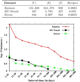
Table 1: Basic statistics of the datasets used in the paper. Dataset |V| |E| |T| Recipro Epinion 131,828 841,373 938 0.3083 MC-Email 167 5,783 237 0.876 Enron 182 3,007 944 0.6053 0 0.5 1 1.5 2 2.5 3 1-10 11-20 21-30 31-40 41-50 51-75 76-100 101-200 201-300 301-400 401-500 log ( # instances )
Interval time (in days) Epinion MC-Email Enron
Fig. 2: Histogram of interval time of reciprocal link.
datasets, we provide the empirical distribution of observed interval time and its goodness of fit with known statistical distributions. For theEnrondataset, the persons (along with their rank in the company) associated to a vertex is known, so in this dataset we have also performed a qualitative study by checking for the evidences of social stratification phenomenon, which we present at the end of this section.
We used three real-world directed network datasets for our study. We se-lected datasets where reciprocal link creation is an important (meaningful) event; another selection criterion is that the datasets should have a sufficient number of reciprocal links to train and test the models (Kuhnt and Brust, 2014). Our first dataset,Epinion is a trust network where a directed link from one vertex to another represents the fact that the former trusts the latter. The RLTP task for this dataset is to find the time at which a trusted person ac-knowledges that (s)he also holds a similar sentiment towards the other person. The dataset was collected from KONECT web page.2 We have also collected two email datasets: MC-Email3 and Enron. Both of these datasets are email communication networks from two distinct enterprises, and for these datasets the RLTP task is to predict the response time for an email. More informa-tion on these datasets is provided in Table 1, where|V|,|E|,|T|, andRecipro
2 http://konect.uni-koblenz.de/networks/
3 This is Manufacturing Company email dataset available from R. Michalski’s website,
are the number of vertices, the number of edges, the number of timestamps (in days), and the reciprocity of the dataset within the observation window, respectively.
For these three datasets, we plot the histogram of the interval time for reciprocal links in log scale (Figure 2). We observed that the majority of the responses are received within a short period of time (within 10 days or less). However, there also exist a few late responders whose reply time is much larger than the average reply time.
3.2.1 Modeling interval time using Parametric Distribution
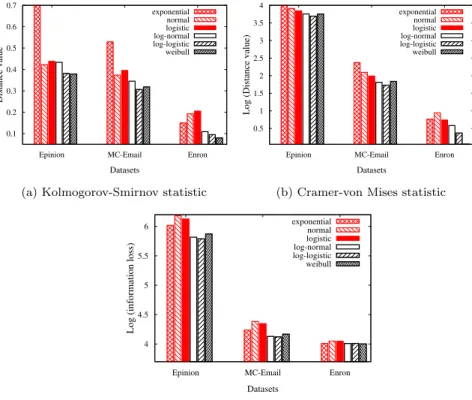
From the distribution plots in Figure 2 we observe that the number of re-ciprocal link instances reduces exponentially with the increment of the in-terval time (note that, y-axis is in log-scale). Hence, we fit different expo-nential family distributions to model the time interval of reciprocal link for all three datasets. Specifically, we fit exponential distribution, normal distri-bution, logistic distridistri-bution, log-normal distridistri-bution, log-logistic distribution and Weibull distribution. To evaluate the goodness of fit we use the
0.1 0.2 0.3 0.4 0.5 0.6 0.7
Epinion MC-Email Enron
Distance value Datasets exponential normal logistic log-normal log-logistic weibull
(a) Kolmogorov-Smirnov statistic
0.5 1 1.5 2 2.5 3 3.5 4
Epinion MC-Email Enron
Log (Distance value)
Datasets exponential normal logistic log-normal log-logistic weibull
(b) Cramer-von Mises statistic
4 4.5 5 5.5 6
Epinion MC-Email Enron
Log (information loss)
Datasets exponential normal logistic log-normal log-logistic weibull
(c) Aikake’s Information Criterion
ing four metrics: Kolmogorov-Smirnov (KS) statistic, Cramer-von Mises (CM) statistic, Aikake’s Information Criterion (AIC) (Akaike, 1998) and Bayesian Information Criterion (BIC) (Schwarz, 1978). In Figure 3, we show the qual-ity of fitting results. The results of BIC are very similar to AIC for all three datasets, so we did not show the results of BIC. As depicted in Figure 3, exponential, normal, and logistic distributions (shown in red) have relatively high distance from empirical distribution compared to log-normal, log-logistic and Weibull distributions (shown in black). For the Enron dataset, Weibull distribution performs the best over all metrics. Similarly, for theEpinion and the MC-Email datasets logistic distribution fits the best. Results of log-normal distribution are very similar to both Weibull and log-logistic distri-butions. Hence, we use log-normal, log-logistic and Weibull distributions for parametric survival models, which are discussed later in Section 3.5.
3.2.2 Social Stratification in Enron
One of the influencing factors for late responses to a specific user is social stratification - particularly in corporations, people tend to give quicker replies to their superior as compared to their colleagues and other juniors. We study the Enron dataset, for which the employee details are available with email communications. In the dataset, “Louise Kitchen” is a president; we observed that her email replying practice follows social stratification phenomenon. She generally takes more than 2−3 days to reply to people with lower ranking positions such as vice-president (VP), employees, etc. For example, she replied to VPs “Kevin Presto”, “James Steffes” and “Fletcher Sturm” in 3, 6 and 19 days respectively. She replied to “Sally Beck” (Chief Operating Officer) in 5 days. On the other hand she replied to “David Delainey” (Chief Executive Of-ficer (CEO)) on the same (0) day. Another example is “Philip Allen”, who is a manager; he replied within a day to higher ranking officers such as “David De-lainey” (CEO), “Barry Tycholiz” (VP), “Hunter Shively” (VP) and “Richard Shapiro” (VP). On the other hand, he took 2 to 3 days to reply to “Michael Grigsby” (manager), “Jay Reitmeyer” (employee) and “Matthew Lenhart” (employee).
3.3 Topological Feature Study
In online social networks, user behavior based features are useful for solv-ing different problems, such as, link prediction (Valverde-Rebaza and de An-drade Lopes, 2013), personality prediction (Adalı and Golbeck, 2014), user attribute prediction (Tuna et al, 2016), link sign prediction (Shahriari et al, 2016), prediction of positive and negative users in Twitter (Roshanaei and Mishra, 2015), etc. Hence, we believe social (behavioral) phenomena based topological features can contribute substantially to solve theRLTP problem. Though there are works that study and design user behavior features such as
topic-specific modeling (Bogdanov et al, 2014), a behavioral model for Face-book wall posts (Devineni et al, 2017), etc., we assume to have only topological information. Topological features that we use comes from two different social phenomena: directed altruism and social stratification. Below we discuss them in two different sections.
3.3.1 Directed Altruism Based Features
Directed altruism in social networks is described in (Leider et al, 2007), where the authors have argued that people are more generous to friends and friends of friends than to a complete stranger. This phenomenon also reflects in people’s reciprocal link creation behavior. Below, we define some topological features which quantify the directed altruism phenomena for reciprocal link prediction.
Shortest directed distance: In our problem, one directional link (v, u) already exists, and we are predicting the creation time for the reverse link (u, v). Generally people are more generous to indirect friends than complete strangers. Henceuis more likely to respond quickly tovfor small value of the directed distance fromuto vi.e.
DirectedDist(u, v) =d(u, v)
Common in/out neighbors count:The number of common neighbors is a frequently used topological feature for the link prediction task in undirected networks; however, for directed graphs, we have two separate features: common in-neighbors and common out-neighbors. Both of these topological features capture the idea that if a user has more common neighbors with another user, then she is more likely to reply fast. Also, more common friends increase the network flow, which is an important factor for building trust (Leider et al, 2007) and with higher trust people tend to reply faster.
Commonin(u, v) =|Γin(u)∩Γin(v)|
Commonout(u, v) =|Γout(u)∩Γout(v)|
Jaccard coefficient (In/Out):The Jaccard coefficient is another widely used topological feature for undirected networks. It is the normalized version of common neighbors counts. Similar to the common neighbor count feature, this feature also split into two features due to the directed-ness of the edges. Jaccard coefficients help to predict the trust level between two nodes. Since, higher trust leads to faster response, this is a good feature for theRLTPtask.
J accardin= |Γin(u)∩Γin(v)| |Γin(u)∪Γin(v)| J accardout= |Γout(u)∩Γout(v)| |Γout(u)∪Γout(v)|
Local Reciprocity. In (Gong and Xu, 2014), the authors studied two local reciprocity features and they showed relative influence of both features
on linking back probability. The first is Acceptance Local Reciprocity (ALR), which is defined as:
ALR(v) =|Γin(v)∩Γout(v)|
|Γin(v)|
We compute ALR for the head node (v) of the reciprocal link (u, v). This feature captures the tendency of node v to accept a link. The second feature is Request Local Reciprocity (RLR), defined as:
RLR(u) =|Γin(u)∩Γout(u)|
|Γout(u)|
We compute RLR for the tail node (u) of the reciprocating link (u, v). RLR
represents the response behavior of the nodeu and captures its tendency to initiate a reciprocal link.
3.3.2 Social Stratification Based Features
It is observed that in online social networks people behave according to their status in the network (Hopcroft et al, 2011). A similar behavior is observed in many real world applications, such as the one described in Section 3.2 or in online dating (Xia et al, 2013). We have also shown evidence of social stratification in Enron dataset, specifically in connection to the RLTP task. The following topological features quantify the extent of social stratification that is practiced by the nodeuor v.
Preferential Attachment:This feature computes a value which reflects the social stratification induced rank order of a given node. The basic idea of preferential attachment is to give more weight to the higher degree nodes. Traditionally, preferential attachment has been computed for undirected net-works, so we change the formula to adapt it for a directed networks. For undirected graph, it is simply the product of the degrees of the nodeuandv. For directed graph, we take the product of the out-degree of the tail node (u) and the in-degree of the head node (v) of a prospective reciprocal link (u, v). The formula is given below:
P ref Att(u, v) =|Γout(u)| × |Γin(v)|
Preferential Jaccard:PrefJacc is inspired by both Preferential Attach-ment and Jaccard Coefficient. It is a trade-off between two concepts—first, high degree nodes are prone to create more edges, and second, nodes prefer to connect with similar nodes (social stratification). Both these phenomena can influence reciprocal edge creation. We calculated PrefJacc by using the following equation:
P ref J acc(u, v) = |Γout(u)∩Γin(v)|
|Γout(u)∪Γin(v)|
In/Out Ratio:A node in the upper hierarchy has a tendency to a create reciprocal edges with other nodes at the same hierarchy level than to nodes
which are at a lower hierarchy level (Hopcroft et al, 2011). To reflect this knowledge in our model, we need to find an efficient way for comparing the hierarchy of a pair of nodes, which we compute by the ratio of their in-degrees and the ratio of their out-degrees. HigherInRatio is indicative of higher ten-dency of the numerator node to attract links compared to the denominator node; similarly, higherOutRatio represents a higher tendency of the numera-tor node to create links compared to the denominanumera-tor node. In this way, these two features capture the relative patterns of link creation and link acceptance by the pair of the vertices. For reciprocating link (u, v), we calculateInRatio
andOutRatio by using the following equations:
InRatio=|Γin(u)|
|Γin(v)| OutRatio= |Γout(u)|
|Γout(v)|
PageRank:PageRankrepresents the prestige of the node in the network. We use both, pagerank ofuand pagerank ofv as features. IfPageRank(u) is lower thanPageRank(v), then the nodeuis highly likely to respond faster to the nodev.
3.3.3 Feature analysis
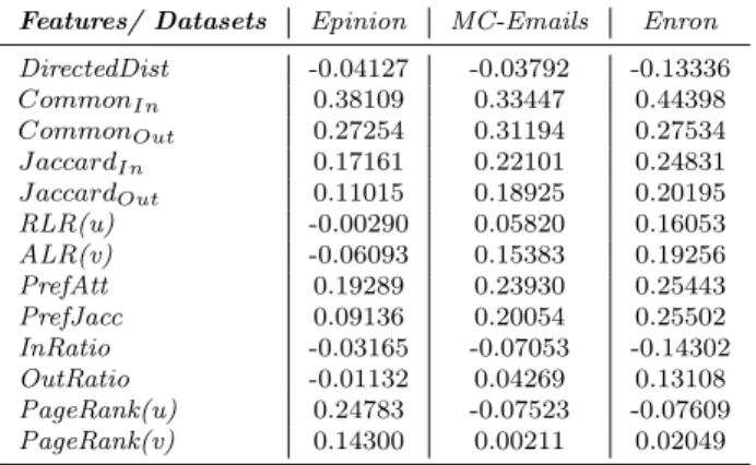
To validate the strength of these features (13 in total) for predicting the in-terval time of reciprocal edges, we compute the Pearson’s correlation of the above topological features with the interval time value for three real-life graph datasets (Table 1) and show the correlation values in Table 2. As we can see, for theMC-Emailsdataset most of the features (mainlyCommonin,Commonout,
J accardIn, J accardOut, PrefAtt and PrefJacc) have good correlation value
(between 0.2 to 0.5). Similarly, for theEnron dataset the same set of features
Table 2: Correlation of features with Interval time
Features/ Datasets Epinion MC-Emails Enron
DirectedDist -0.04127 -0.03792 -0.13336 CommonIn 0.38109 0.33447 0.44398 CommonOut 0.27254 0.31194 0.27534 J accardIn 0.17161 0.22101 0.24831 J accardOut 0.11015 0.18925 0.20195 RLR(u) -0.00290 0.05820 0.16053 ALR(v) -0.06093 0.15383 0.19256 PrefAtt 0.19289 0.23930 0.25443 PrefJacc 0.09136 0.20054 0.25502 InRatio -0.03165 -0.07053 -0.14302 OutRatio -0.01132 0.04269 0.13108 PageRank(u) 0.24783 -0.07523 -0.07609 PageRank(v) 0.14300 0.00211 0.02049
0 0.005 0.01 0.015 0.02 0.025 0.1-5 5.1-10 10.1-1515.1-2020.1-2525.1-3030.1-4040.1-5050.1-6060.1-7070.1-8080.1-100
Linking back Probability
In Ratio 0 0.002 0.004 0.006 0.008 0.01 0.012 0.014 0.016 0.018 0.1-1.11.2-2.22.3-4 4.1-5.55.6-7.37.4-9.59.6-12 12.1-1414.1-15.515.6-1818.1-2525.1-2828.1-30
Linking back Probability
Out Ratio
Fig. 4: Relation ofIn/OutRatioand linking back probability inEpiniondataset
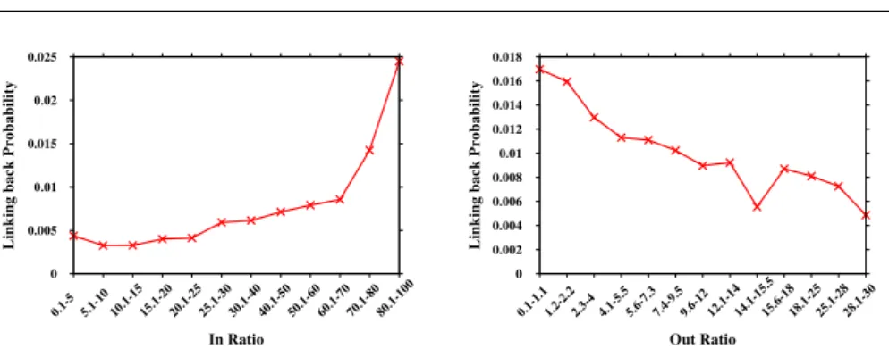
is highly related to interval time. But, for Epinion dataset the correlation values for most of the features are poor except for Commonin,Commonout, andPageRank(u); the worst features areInRatio, OutRatio andRLR(u). To check the influence of these features on reciprocal link creation, we also check the average linking back probability over different range of values for different features. We discuss our observation in the following paragraphs.
In Figure 4, we plot our observation for two of the features: InRatio and
OutRatio. Here, for each bin ofInRatio, the linking back probability is calcu-lated as a fraction of reciprocal links over all the links in that bin. Figure 4 clearly shows high linking back probability for higherInRatio and lower Out-Ratio, which is expected behavior for these features. In (Gong and Xu, 2014), the authors provided a thorough study of some features, such as,RLR(u)and
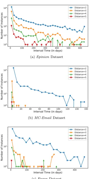
ALR(v), and proved their significant influence on reciprocal link creation. in Figure 5, we show three plots (one for each dataset) ofDirectedDist vs. interval time. Within each plot we have several graphs, each representing the directed distance value between the vertices. Along the x-axis is the interval time and along the y-axis is the number of reciprocal link instances that have the corresponding interval time. For all dataset, we observe that links with small directed distance value (such as, 2 or 3) can have high interval time, i.e. the reciprocal link may appear after many days; but as distance increases there are few or almost no instances of reciprocal links with high interval time. This observation may appear counterintuitive as we expect short distance to influence a short interval time. However, This observation can be explained as follows: people tend to trust other people who are within their circles, and they will ultimately create a reciprocal links with them, even if they do not do it immediately. On the other hand, for people who are outside someone’s circle (having a high directed distance value, such as 4 or 5), reciprocal links will be created either in a short interval time or will not be created at all. The short interval time can be the cases when two strangers meet in-person in a social event and then mutually agree to be connected online (or trust each other). On the other hand, the negative case happens, when a stranger trusts (or sends an invite to) someone, and the second person just ignore that forever. Due to
0 100 200 300 400 500 600
Interval Time (in days)
100 101 102 103 104 Nu mb er of Inst an ce s Distance=2 Distance=3 Distance=4 Distance=5
(a)EpinionDataset
0 20 40 60 80 100 120 140 160
Interval Time (in days)
100 101 102 103 Nu mb er of Inst an ce s Distance=2 Distance=3 Distance=4 Distance=5 (b)MC-EmailDataset 0 100 200 300 400
Interval Time (in days)
100 101 Nu mb er of Inst an ce s Distance=2 Distance=3 Distance=4 Distance=5 (c)Enron Dataset
Fig. 5:DirectedDist vs. Interval Time
this complex relation, the correlation between directed distance and interval time is poor, yet we considerDirectedDist to be a useful feature.
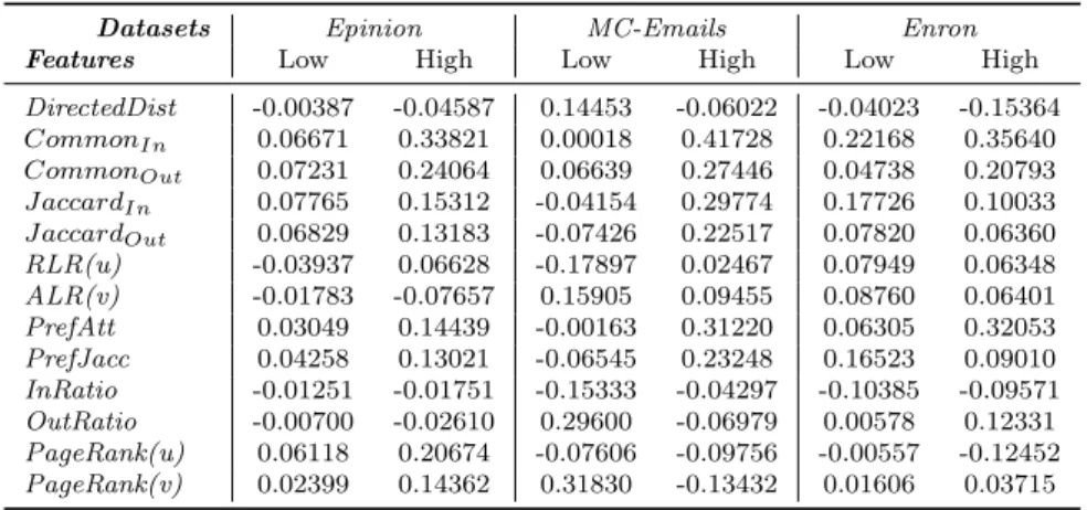
Correlation with Low and High Interval time.
There are a variety of different social behaviors that influence the interval time, hence some social based features impact the interval time differently over a period. To understand the impact of different features over a period, we split the target variable (interval time) into lower and higher range and
Table 3: Correlation of features with Low and High Interval times
Datasets Epinion MC-Emails Enron
Features Low High Low High Low High
DirectedDist -0.00387 -0.04587 0.14453 -0.06022 -0.04023 -0.15364 CommonIn 0.06671 0.33821 0.00018 0.41728 0.22168 0.35640 CommonOut 0.07231 0.24064 0.06639 0.27446 0.04738 0.20793 J accardIn 0.07765 0.15312 -0.04154 0.29774 0.17726 0.10033 J accardOut 0.06829 0.13183 -0.07426 0.22517 0.07820 0.06360 RLR(u) -0.03937 0.06628 -0.17897 0.02467 0.07949 0.06348 ALR(v) -0.01783 -0.07657 0.15905 0.09455 0.08760 0.06401 PrefAtt 0.03049 0.14439 -0.00163 0.31220 0.06305 0.32053 PrefJacc 0.04258 0.13021 -0.06545 0.23248 0.16523 0.09010 InRatio -0.01251 -0.01751 -0.15333 -0.04297 -0.10385 -0.09571 OutRatio -0.00700 -0.02610 0.29600 -0.06979 0.00578 0.12331 PageRank(u) 0.06118 0.20674 -0.07606 -0.09756 -0.00557 -0.12452 PageRank(v) 0.02399 0.14362 0.31830 -0.13432 0.01606 0.03715
calculate feature correlations with lower and higher interval times separately. For this study, we calculate average interval time for each dataset and if the interval time is less or equal to average interval time we call it low interval time, otherwise, we call it high interval time. For each dataset and each feature we calculate the correlation value between the feature and low and high interval times; these correlation values are shown in Table 3.
In Table 3, we observe that features likeCommonin,Commonout,J accardIn,
J accardOut, PrefAtt andPrefJacc have high correlation with higher interval
time. For the Enron dataset, some of these features (Commonin,J accardIn and PrefJacc) are highly correlated to lower interval time as well. For the
MC-Email dataset, DirectedDist, ALR(v), Out Ratio and PageRank(v) have noticeable correlation with lower interval time and other two features (RLR(u)
and In Ratio) are inversely correlated to lower interval time. One surprising observation for theMC-Email dataset is thatPageRank(v)is the poorest fea-ture (Table 2), but highly correlated with both lower and higher interval times, mainly because the feature is positively correlated for lower interval time and inversely correlated with higher interval time. From Table 3 we understand that for different datasets user behavior varies and hence a distinct set of fea-tures becomes influential to the interval time (especially lower interval time) of that dataset.
3.4 Proposed methodology using survival analysis
Survival analysis is widely used in the medical domain to predict survival time or time to a specific event (such as death) for patient datasets (Vinzamuri and Reddy, 2013), (Wang et al, 2017a). In the survival analysis setup, for a set of instances under observation, events happen over a time period, from which a survival model learns the temporal patterns of these events and predicts the survival time. Here, we propose a novel method to map the RLTP problem
to a survival analysis task and explain survival analysis concepts from a re-ciprocal link creation perspective. For these concepts, we also provide suitable terminology for theRLTP problem to describe our approach clearly.
Beginning of graph expansion and study period: At the first time-stamp, a given directed time-stamped network is static (initialized); the be-ginning of graph expansion is the second time-stamp from when new links are added to the static network. Survival analysis assumes a starting time of the study, from when a model starts to observe for the events. In the RLTP problem, thebeginning of graph expansion serves as the starting time of the study. For theRLTP problem, we divide the time-stamps of the network into train and test time periods, and we observe the network for the reciprocal link creation till the end of the train period, so the last time-stamp in the train period is considered to be theend of the study. Thus the time window from the beginning of graph expansion to the last time-stamp of train period is considered to be thestudy periodwhich is the same as the train period.
Reciprocal event: For a parasocial link (v, u), if a reciprocal link (u, v) is created during the training period, we call it a reciprocal event, which is the event of interest in theRLTPproblem. In theRLTP problem each parasocial link is a data instance, time-stamp of a parasocial link generation is the time when the data instance is considered into the network for study. Hence, the time-stamp of a parasocial link generation is called thestarting time of ob-servationfor that data instance (an ordered pair of vertices).
ever-waiting links: We study the network for a limited time window (train period), and hence for a set of parasocial links, the corresponding reciprocal event may not be observed before the end of the study (last time-stamp of training period). We call these linksever-waiting links.ever-waitinglinks carry the information that the reciprocal link creation event did not happen till the end of the train period. In the survival analysis terminology the ever-waiting links are also called censored instances; we use both of these terms interchangeably in this paper.
In a traditional regression task, ever-waiting links may either be ignored, because the target value (the interval time) for these instances are unknown, or they may be retained with an arbitrarily chosen large interval time, which is higher than the time difference between the end of the study time and the starting time of observation for that parasocial link. The first of the above ap-proaches ignores important information; specifically, the ignored fact is that the interval time forever-waiting links is higher than the time difference be-tween the end of the study and the starting time of observation for that paraso-cial link. The second approach is simply a crude approximation of the target value. As mentioned before, the main reason to map theRLTP problem into survival regression analysis framework is to exploit the important information provided by theever-waiting links.
Target value of survival regression model:The time difference between the starting time of observation (parasocial link generation time) and the time-stamp of the reciprocal edge creation is the interval time which we want to predict in the RLTP task. For a reciprocal edge (u, v), the interval time is defined as Int(u, v), as is discussed in Section 3.1. In a traditional survival model, the interval time is called the life-span of an instance as for these mod-els “death” is the event of interest. Hence survival modmod-els that predict survival time can be adopted to predict the interval time for theRLTP problem. For training the prediction model, we need a feature vector for each data instance, along with the survival time and a binary event indication value (event oc-curred or not). For theRLTP problem, the feature vector of a parasocial edge isxi∈Rd, a vector of topological features (Section 3.3) for thei’th parasocial
link in training data, where feature dimension dis 13 (number of topological features). For each parasocial links of the training period, if the reciprocal event has occurred during training period then life-span of parasocial link is the interval time with the event indication value set to 1; otherwise, for ever-waiting links, the time difference between the last time-stamp of training and time-stamp of the parasocial link generation is the survival time with event indication value set to 0. Given this training dataset the target value (the in-terval time) of test instances are predicted by using a trained survival model. We use various survival models, which we discuss in the next subsection.
3.5 Survival models for theRLTP problem
As explained in the previous section, any survival model can be adopted to solve theRLTPproblem. There are two types of widely used survival models: 1) semi-parametric models and 2) parametric models. Parametric models as-sume that interval time follows a known statistical distribution; hence, if the in-terval time for a dataset follows a distribution then parametric models perform very good for the dataset compared to a semi-parametric models. However for many real-world datasets, it is difficult to find a suitable statistical distribution that fits well to the interval time, for these datasets semi-parametric models perform better than parametric models, because semi-parametric models do not assume any underlying distribution, rather they try to learn the actual dis-tribution from the data. As we discussed in Section 3.2, some of our datasets are good fit for a statistical distribution but others are not. Hence, we con-duct experiments with both semi-parametric and parametric models to offer a comprehensive study of the RLTP problem. In this section, we describe these selected semi-parametric and parametric models and their adaptation for solving theRLTP problem. Broadly, all types of models try to predict the survival time of an instance in the data by modeling three functions: 1) Sur-vival function, 2) Hazard function and 3) Event density function. Definitions and relationship between these three functions are described below:
Survival functionS(t) Survival models provides a principled approach for in-terval time prediction by modeling a survival function, which is defined as the probability value that the reciprocal edge creation does not happen for a given parasocial link before a specified timet.
S(t) =P r(T ≥t)
Here,T is a random variable representing the time of the reciprocal edge cre-ation event.
Hazard functionλ(t) is the reciprocal event rate at timet conditional on the fact that the reciprocal event has not occurred until that timet,
λ(t) = f(t)
S(t) (1)
wheref(t) is thereciprocal event density function, which is given as follows:
f(t) = d
dt(1−S(t)) =− d dtS(t)
For a given parasocial link if corresponding reciprocal link is not likely to be created at timet then Survival function value for t is high. On the other hand, if the corresponding reciprocal link is highly likely to be created at time tthen thereciprocal event density functionvalue should be high and that leads to a higher value of the Hazard function. We can observe that both survival function and hazard function are interrelated and we can model either func-tion for the interval time predicfunc-tion. Next, we describe how semi-parametric Cox regression models thehazard function to solve theRLTP problem. Later we discuss parametric methods (BJ-model and AFT models) and their ap-proach for modeling thesurvival function with the help of different statistical distributions.
3.5.1 Cox Regression
Cox regression model (Cox, 1972) is the most widely used semi-parametric model for predicting the (interval) time taken for a reciprocal event to occur. The basic Cox model follows the proportional hazard assumption, for which the hazard functionλ(t|xi) takes the following form:
λ(t|xi) =λ0(t)×exp(β1xi1+β2xi2+...+βdxid) =λ0(t)×exp(xTiβ)
(2)
where, xi is the (topological) feature vector of a parasocial link represented as i’th data instance in the training data and dis the dimensionality of the features. Here, λ0(t) is called baseline hazard function, and β is the model parameter which Cox regression model learns. The Cox regression is called semi-parametric because the baseline hazard function λ0(t) can be any non-negative function of time. The probability of occurrence of reciprocal event for
the ith parasocial link (data instance) at time t can be represented as ratio λ(t|xi)
P
j∈Rtλ(t|xj), whereRtis the set of all instances for which the reciprocal event
did not happen until t. The product of these probabilities gives the partial likelihood function: L(β) = N Y i=1 " exp(xTiβ) P j∈Rtexp(x T jβ) #Ci (3)
Here, N is the total number of parasocial links appeared during the training period and Ci is an event indicator value, i.e., if reciprocal link for the ith parasocial link appear during training period then Ci = 1 otherwise Ci = 0. The model parameter β is learnt by minimizing the negative log likelihood function. Ifβbis the optimal model parameter, we have:
b β= argmin β 1 N N X i=1 −Ci(xTiβ) +Cilog X j∈Rt exp(xTjβ) (4)
Regularized Cox model: For complex model with high dimensional real world datasets, over-fitting is a frequent problem. To avoid this, we need a regularization term in the objective function (Equation 4). We observe in Section 3.3.3 that only a few features have a strong correlation with the target variable, so we want to use a sparse regularization model. In this work we use Elastic Net regularization. In literature, a Cox model with Elastic Net regularization is also known as Cox model with Elastic Net (EN) penalty (Zou and Hastie, 2005). The penalty termPEN is:
PEN(β) = d X k=1 α|βk|+ 1 2(1−α)β 2 k (5)
Where, 0< α≤1 and with EN penalty the objective function in Equation 4, becomes b β= argmin β 1 N N X i=1 −Ci(xTiβ) +Cilog X j∈Rt exp(xTjβ) +γ·PEN(β) (6)
Here,γ >0 is a regularization constant. For solving this optimization task, we can use the maximum partial likelihood estimator proposed in (Cox, 1972); it uses the Newton-Raphson method to iteratively find the estimated βb which minimizes the Equation (6).
3.5.2 Parametric Models
The main idea behind a parametric model is that it assumes that the interval time follows a specific statistical distribution. There are two ways to relate interval time and a statistical distribution: first, assume that the actual interval time for all parasocial links follows a distribution; and second, assume that the logarithm of the interval time follows a distribution. The models under the first assumption are referred to as linear regression models, and the models under later assumption are called accelerated failure time (AFT) models.
Generally, parametric models use maximum likelihood estimation (MLE) approach to learn model parameters. Let’s assume all the parameters of a model are represented by β = (β1, β2, ...)T. For a given parasocial link (say ith link in the training data), if it is an ever-waiting link the corresponding survival functionS(t,β) at timet(in fact, anytvalue during a training period) should be near to 1, and if it is not an ever-waiting link then the reciprocal event density functionf(ti,β) at timeti (time of reciprocal event for the ith parasocial link) should be high (near to 1) for that link. Hence, the likelihood of all parasocial links of a training period is the product of their reciprocal event density functions or survival functions based on their state (whether the link isever-waiting or not), i.e.
L(β) = Y Ci=1 f(ti,β)· Y Ci=0 S(ti,β) (7)
Linear regression model: The statistical linear regression with the least squares estimation is widely used for a variety of regression tasks. However, the issue with the model is that it cannot use information from ever-waiting
links. For interval time prediction this issue can be handled by using a spe-cific survival model such as the Buckley-James model (BJ model). The BJ model first estimates the interval time of trainingever-waiting links using the Kaplan-Meier (KM) (Kaplan and Meier, 1958) estimation method and then by using all parasocial links from training period to train a linear model. This linear model can be trained through MLE as described above. For more prac-tical use, Wang et al. (Wang and Wang, 2010) proposed twin boosting method with BJ estimator, we use this method to solve theRLTP problem.
Accelerated Failure Time (AFT) model: An AFT model assumes that the logarithm of the interval time log(T) follows a statistical distribution and it is linearly related to the (topological) feature vectors. The general form for AFT regression model is
log(T) =X·β+σ· (8)
whereX is the covariate matrix of sizeN×dwhereithrow ofX isxi,βis a ddimensional coefficient vector (model parameters),σ(σ >0) is an unknown scale parameter, andis an error variable which follows a similar distribution
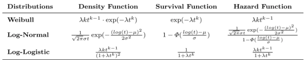
Table 4: Density, Survival and Hazard functions for the distributions used with AFT model.λis scale parameter andk is shape parameter for both Weibull and log-logistic distribution. For log-normal distributionµis the mean (loca-tion parameter), σ2 is the variance andΦis cumulative distribution function of normal distribution.
Distributions Density Function Survival Function Hazard Function Weibull λktk−1·exp(−λtk) exp(−λtk) λktk−1
Log-Normal √1 2πσtexp(− (log(t)−µ)2 2σ2 ) 1−Φ( log(t)−µ σ ) 1 √ 2πσtexp(− (log(t)−µ)2 2σ2 ) 1−Φ(log(σt)−µ) Log-Logistic λktk−1 (1+λtk)2 1+1λtk λkt k−1 1+λtk
to log(T). For our problem, we use the three most suitable distributions (see Figure 3) for interval time, the details of which are given in Table 4.
3.6 Algorithmic framework
In Algorithm 1, we describe a general framework of our proposed method. First we divide the time-stamps of the input graph into train and test periods as mentioned in line 1 of Algorithm 1. After that we create training data instances (train-set) and test data instance (test-set) from the corresponding train and test periods (Lines 2-4). Then we calculate topological features for each parasocial link (data instance) in thetrain-setandtest-setas described in Lines 5-10 of Algorithm 1. After that we generate target variable for each data instance (Lines 11-26), for which we observe the corresponding reciprocal link in the graph. For a parasocial linke∈train-set, if the corresponding reciprocal link is generated during train period then interval time Int(e) (Section 3.1 ) is the target value with event indicator valueCe= 1 otherwise time difference between the link creation and end of training period act as the target value with event indicator valueCe= 0. Similarly, we generate target values for data instance of test-set as explained in Lines 27-35 of Algorithm 1. Then, we use R libraries to train the survival models with training data and predict target values for the test data to generate the test results (test-res) and lastly we evaluate thattest-res.
4 Experiments and Results
We conducted a set of rigorous experiments to demonstrate the benefit of using censored information and the superiority of proposed survival models to solve the RLTP problem. We used five proposed survival models: Cox regression model, AFT model with Weibull, log-normal and log-logistic distributions, and Buckley-James (BJ) regression model. To prove the fact that the proposed survival models are better suited for solving theRLTPproblem, we compared
Algorithm 1Our Framework
1: For time-stamps (t0 totM) of the input graph, divide the startingp% time-stamps as
training period (t0-tp) and remaining as testing period (tp+1-tM).
2: train-set←all parasocial links generated before/at time-stamptp.
3: test-set←all parasocial links generated after time-stamptpand immortal links.
4: Sort edge intrain-setandtest-setbased on its edge creation time. {optional}
5: for each(edge)e∈train-setdo
6: Gte←create a snapshot of the network atte−1. {sorting helps in this step}
7: xe←generate topological features (Section 3.3) for edgeefrom the snapshotGte.
8: addxe toX.
9: end for
10: Similarly, generate topological features for edges in thetest-setand generateXtest. 11: for eache∈train-setdo
12: ifehas a reciprocal linker in datasetthen
13: if ter≤tpthen
14: ye←Int(e)←ter−te {target value for the parasocial edge (data instance)}
15: Ce←1 {event indicator value for the parasocial edge (data instance)}
16: else
17: ye←tp−te {target value for theever-waiting link (data instance)}
18: Ce←0
19: end if
20: else
21: ye←tp−te {target value for theever-waiting link (data instance)}
22: Ce←0
23: end if
24: addyetoT.
25: addCe toC.
26: end for
27: for eache∈test-setdo
28: ifehas a reciprocal linker in datasetthen
29: ye←Int(e)←ter−te {target value for the parasocial edge (data instance)}
30: Ce←1
31: else
32: ye←tM−te {target value for theever-waiting link (data instance)}
33: Ce←0
34: end if
35: addyetoTtest.
36: addCe toCtest.
37: end for
38: {Use one of the methods among Cox, BJ, and AFT; below we call all three methods}
39: cox←cocktail(X,T,C) {method off astcox(Rpackage)}
40: {For given distributiondist}
41: AF Tdist←survreg(X,T,C,distribution=dist) {method ofsurvival(Rpackage)}
42: BJ model←bujar(X,T,C) {method ofbujar(Rpackage)}
43: Thecox,AF TdistandBJ modelcontain the model parametersβ.
44: test-res←predict interval timeyefor each edgee∈test-setusingXtestandβ.
45: evaluatetest-resusingTtestandCtest.
them with traditional regression models such as ridge regression (RidgeReg), lasso regression (LassoReg), feed forward neural networks (FFNN) and support vector regression (SVR). Note that these traditional regression models cannot use censored information (ever-waiting links). We also compare proposed Cox regression model with generalized linear model (GML), which is an adopted model from (Sun et al, 2012).
In addition to the suitability of the proposed survival models for theRLTP problem, we also demonstrate the usability of theever-waiting links. For that, we conducted experiments where we train the survival models without cen-sored information and compare the performance of the models on the test dataset. We report the improvement in the performance when theever-waiting
links are used for training the survival models.
Lastly, we conduct an experiment to show that reciprocal links with short interval time contain enough information required for training the survival models.
4.1 Datasets
For the experiments, we use three real world datasetsEpinion,MC-Email and
Enron. We discuss these datasets in Section 3.2 and basic statistics of the datasets are shown in Table 1.
Generating a synthetic dataset for the RLTP problem is a challenging task, because in the literature most of the synthetic graph generation models try to mimic basic real-world properties such as power-law degree distribu-tion (Faloutsos et al, 1999), community structures (Leskovec et al, 2007), etc. All these methods generate directed networks with extremely low reciprocity— generally, less than 1%. Durak et al. have proposed a synthetic network gener-ation algorithm which also considers reciprocity (Nurcan Durak, 2013). We use this algorithm for generating three synthetic graphs where the vertex count varies between 10,000 (10K) to 30,000 (30K) with increments of 10K. Edges of these synthetic networks have no time-stamps; hence, we assign random time-stamps between 0 to 100 to parasocial links. The time-stamps of recip-rocal links of these synthetic networks are selected by matching the reciprecip-rocal link interval time of theEpinion dataset through the best fit Weibull distri-bution.
4.2 Experimental Setting
For our experiments, we divide the time-stamps of a dataset into two non-overlapping continuous partitions, where the earlier partition is the train pe-riod and the latter is the test pepe-riod. In three different experiments, we use, respectively, 60%,70% and 80% of the earlier time-stamps as the train peri-ods and the remaining time-stamps as the test period. For synthetic datasets, a 70:30 split of the time-stamps is used as the train and test period of our experiments. For calculating the topological features explained in Section 3.3 for a parasocial link (data instance), we take a snapshot of the network until the time-stamp of the corresponding reciprocal link or end of the train period (whichever is earlier).
Like any other link prediction task, RLTP also suffers from the class im-balance issue, where the number of positive instances (Ci= 1) is much smaller
than that of the negative instances. To alleviate this problem we use the well-known majority undersampling (Bunkhumpornpat et al, 2011) strategy as discussed below: all the reciprocal links generated during a train period are considered in the training data pool as positive instances and only 50% of the parasocial links generated during the same period are censored negative instances (Ci = 0) in the pool. The test data pool (and their labels) are also generated similarly from the test period. As train and test data instances need to be from their corresponding time periods, we use a modified K-fold cross validation, where each fold contains a random subset of train and test data instances from their respective pools. For all our experiments, we used 5-fold cross validation in this manner.
For minimizing the objective function (Equation (4)) of censored prob-lem formulation of RLTP, for the Cox regression model, we used cocktail algorithm (Yang and Zou, 2013) (the library is provided by the authors of (Yang and Zou, 2013)). For AFT models and BJ regression, we usedSurvival
package5andBujar package6, respectively, available inR. For RidgeReg, Las-soReg and SVR, we used scikit-learn python library and for FFNN, we used Matlab NNtoolbox. We used TopCom indexing method (Dave and Hasan, 2015, 2016) to find shortest directed distance feature. To choose the best pa-rameters of SVR, we used grid search, where the cost parameter C takes values from {0.0001,0.001,0.01,0.1,1.0} and Epsilon () takes values from
{0.0001,0.001,0.01,1.0}.
4.3 Evaluation Metrics
Datasets generated from directed time-stamped networks are longitudinal data and for the RLTP problem the datasets also contain censored information. Evaluating models on these datasets using traditional evaluation metrics is not suitable, instead we use time-dependent AUC (also known as c-Index), which is widely used in longitudinal data analysis (Pencina and D’Agostino, 2004).
For a pair of data instances, assume (yi, yj) and (ybi,ybj) are the target and the predicted values, respectively. The time-dependent AUC is defined as the probability of ybi >ybj given yi > yj. If target yi has only 2 possible values, then time-dependent AUC is the same as the popular AUC (Area Under ROC Curve) metric for classification. Similar to the AUC metric, time-dependent AUC takes values between 0 to 1, where 1 is the best possible value for this metric. Time-dependent AUC (TD-AUC) is calculated as follows:
T D-AU C= 1 Ncnt X i:Ci=1 X yj>yi 1(ybj>ybi) (9) where, Ncnt is total count of (yi,yj) pairs such that Ci = 1 (the event has occurred) andyj > yi holds.
5 cran.r-project.org/package=survival
For the Cox regression model, the predicted value is the hazard value and for a higher hazard value the event occurs earlier, hence the time-dependent AUC for Cox can be calculated as:
T D-AU C= 1 Ncnt X i:Ci=1 X yj>yi 1(xTi βb>xTjβb) (10)
4.4 Comparison results of survival models and regression models
We compared proposed survival models with four other traditional regression models and our results are shown in Tables 5, 6 and 7, where columns rep-resent different training splits and each row reprep-resents a prediction model. A horizontal bar separates the traditional regression models in the upper part and the survival based models in the lower part. Here, each table cell shows mean and standard deviation for TD-AUC values. For most of the cases, the Cox regression model performs the best.
For the Epinion dataset, as depicted in Table 5, the Cox regression model performs the best with mean TD-AUC 0.7364, 0.7463 and 0.7485 for training period with 60%, 70% and 80% splits of time-stamps, respectively. Here, with increase in the training data we can clearly see improvement in the perfor-mance, which is an expected behavior because with more training examples the model learns better. BJ model is the next best with performance very close to the Cox model. For this model also, the mean TD-AUC improves from 0.7312 to 0.7416 as we increase the training data. Similar behavior is observed for other survival models, but the performance of the AFT models is, unfortunately, not good for the dataset. This can be attributed to the fact that AFT models make strict distribution assumptions on the data and such assumption may not be suitable for theEpinion dataset (Figure 3).
For the Epinion dataset, among the traditional regression based methods, ridge regression performs better than any other competing methods with mean TD-AUC in the range between 0.60 and 0.61. But, when we compare its per-formance over different training splits, we see that its perper-formance does not
Table 5:Epinion Dataset: TD-AUC results [mean (±standard deviation)] with different splits used for training period.
Method / Split 60% 70% 80% RidgeReg 0.6185 (±.0018) 0.6086 (±.0013) 0.6060 (±.0018) LassoReg 0.6169 (±.0013) 0.6020 (±.0014) 0.6039 (±.0017) FFNN 0.5510 (±.1296) 0.5048 (±.0822) 0.4456 (±.0725) SVR 0.4791 (±.0005) 0.4871 (±.0039) 0.4914 (±.0030) BJ Model 0.7312 (±.0010) 0.7339 (±.0020) 0.7416 (±.0021) Weibull 0.3807 (±.0763) 0.5210 (±.1446) 0.5232 (±.1282) logNormal 0.3660 (±.0388) 0.4461 (±.0283) 0.4283 (±.0305) logLogistic 0.4901 (±.0098) 0.5110 (±.0196) 0.5132 (±.0188) Cox 0.7364(±.0025) 0.7436(±.0016) 0.7485(±.0028)
Table 6:MC-Email Dataset: TD-AUC results [mean (±standard deviation)] with different splits used for training period.
Method / Split 60% 70% 80% RidgeReg 0.6213 (±.0087) 0.6083 (±.0146) 0.6014 (±.0125) LassoReg 0.5884 (±.0100) 0.5709 (±.0201) 0.5686 (±.0074) FFNN 0.4199 (±.0800) 0.4609 (±.0964) 0.5069 (±.0915) SVR 0.5462 (±.0154) 0.5737 (±.0187) 0.5530 (±.0150) BJ Model 0.5898 (±.0087) 0.5910 (±.0146) 0.6103 (±.0059) Weibull 0.6139 (±.0075) 0.6171 (±.0069) 0.6315 (±.0166) logNormal 0.6391 (±.0053) 0.6463 (±.0015) 0.6695 (±.0116) logLogistic 0.6380 (±.0121) 0.6494 (±.0062) 0.6747 (±.0201) Cox 0.6527(±.0097) 0.6558(±.0125) 0.6797(±.0062)
Table 7:Enron Dataset: TD-AUC results [mean (±standard deviation)] with different splits used for training period.
Method / Split 60% 70% 80% RidgeReg 0.5732 (±.0073) 0.5847 (±.0159) 0.5318 (±.0164) LassoReg 0.5740 (±.0076) 0.5850 (±.0152) 0.5309 (±.0178) FFNN 0.4900 (±.0258) 0.5407 (±.0434) 0.5363 (±.0561) SVR 0.5490 (±.0080) 0.5680 (±.0176) 0.5608 (±.0136) BJ Model 0.5292 (±.0120) 0.6096 (±.0076) 0.5599 (±.0121) Weibull 0.5710 (±.0168) 0.6319(±.0050) 0.5980(±.0096) logNormal 0.5713 (±.0146) 0.6146 (±.0097) 0.5862 (±.0129) logLogistic 0.5787 (±.0171) 0.6224 (±.0069) 0.5917 (±.0101) Cox 0.5854(±.0166) 0.6311 (±.0110) 0.5919 (±.0084)
improve as we increase the training data. The same behavior holds for other traditional regression methods, such as Lasso regression and FFNN. One pos-sible explanation for this behavior is model under-fitting; that is, the majority of the errors in the traditional regression models are coming from the bias error, so the error does not improve much with a larger dataset which re-duces variance error only. On the other hand, survival analysis based models are more sophisticated, which enables them to design complex functions for predicting the time, thus overcoming the under-fitting issue.
For theMC-Emaildataset, the overall behavior of the models is very simi-lar to theEpinion dataset. Here again the Cox regression model performs the best with mean TD-AUC between 0.65 and 0.68 and its results are improved for larger training data. Performance of different AFT models vary, but they all perform better than all of the traditional regression methods. In particu-lar, AFT with log-logistic and log-normal distributions perform great and their mean TD-AUC is very close to the results of the Cox regression as shown in Table 6. The performance of all survival models improve as we provide more training data. On the other hand, best among the competing methods is ridge regression with a mean TD-AUC between 0.60 and 0.62. As we have discussed earlier, this model suffers from under-fitting problem.
Table 8: TD-AUC results [mean (±standard deviation)] for various methods on synthetic datasets. Method 10K 20K 30K RidgeReg 0.5210 (±.0029) 0.4949 (±.0018) 0.5203 (±.0023) LassoReg 0.5150 (±.0034) 0.4876 (±.0059) 0.5091 (±.0048) FFNN 0.4999 (±.0517) 0.4967 (±.0151) 0.5068 (±.0631) SVR 0.5379 (±.0021) 0.4963 (±.0026) 0.5473 (±.0015) BJ Model 0.5589 (±.0011) 0.5232 (±.0013) 0.5557 (±.0008) Weibull 0.5641 (±.0036) 0.4954 (±.0027) 0.5559 (±.0015) logNormal 0.5670(±.0027) 0.4991 (±.0030) 0.5618(±.0011) logLogistic 0.5597 (±.0029) 0.4985 (±.0042) 0.5576 (±.0019) Cox 0.5604 (±.0025) 0.5282(±.0026) 0.5558 (±.0016)
For theEnron dataset, results are shown in Table 7. Here, for the training period with 60% split, Cox regression performs the best with mean TD-AUC 0.58. For the other two splits, AFT model with Weibull distribution performs the best with mean TD-AUC 0.63 and 0.59. The BJ model performs poorly compared to the other survival models with mean TD-AUC ranging from 0.52 to 0.6, but the performance of BJ model is still better than all competing re-gression methods for training period with 70% and 80% splits of time-stamps. For this dataset, for 80% training split, none of the models have better per-formance than the other splits. This is due to the fact that this dataset is extremely sparse and it has only 3,007 links created during 944 time-stamps (Table 1). Hence even the 80% split does not provide more informative training samples to perform good prediction on remaining data.
The results for synthetic networks are shown in the Table 8 by using the mean TD-AUC and standard deviation metrics. As we observe the results in this table, We can easily conclude that survival models always perform better than traditional regression methods. For two datasets with 10K and 30K node instances, the AFT model with log-normal distribution performs the best among all, while for the dataset with 20K nodes the Cox regression performs the best. The performance of survival models is consistently very similar except for dataset with 20K node where Cox and BJ models clearly perform better than AFT models. Among competing methods, SVR always performs better than others.
4.4.1 Comparison with GLM
Sun et al. (Sun et al, 2012) proposed a method to predict link generation time in a heterogeneous network, where they design a unique feature for the task and use the feature with generalized linear model (GLM) for the prediction task. This proposed feature is designed based on meta-path (a simple path with link label information) in a heterogeneous network. We adopted this feature for a homogeneous network and the adopted feature can be described as a number of simple paths of size k between two nodes. Counting the number
Epinion
MC-Email
Enron
Datasets
0.50
0.55
0.60
0.65
0.70
0.75
0.80
TD
- A
UC
GLM cox regressionFig. 6: Comparison of GLM and cox regression
of simple paths is an extremely costly operation especially for a large dataset such as theEpinion network; hence for this experiment, we usek upto 5 i.e. k ∈ {2,3,4,5} for all three networks, Epinion, MC-Email and Enron. We provide these homogeneous feature values to GLM (with gamma distribution) to solve the RLTP problem. For this experiment we use a 70% split of time-stamps as train period and remaining 30% as test period. The results of this experiment are depicted in Figure 6, where GLM is compared with the Cox regression model for all three datasets. From Figure 6, we observe that the Cox regression outperforms the GLM model for all three datasets by noticeable margins. We believe, one of the main reasons for the poor performance of the GLM based method is that the feature proposed by Sun et al (2012) is carefully designed for an author-paper based heterogeneous network and its adoption in a homogeneous network is not very useful.
4.5 Importance ofever-waiting links
We conducted experiments to show the importance of ever-waiting links and the results are depicted in Tables 9 and 10. Table 9 shows the increment in TD-AUC up to 62% in the real-world datasets, when the survival models are provided with censored information (ever-waiting links) during the training, as compared to when the models are trained without censored information. For theEpinion dataset, the increment in the results is significant (more than 27% for all models) except AFT with log-normal distribution. Similarly, for the MC-Email and the Enron datasets the increment is up to 27%, which is substantial. As shown in Table 10, for the synthetic datasets we also have very similar increment in the results except for the BJ model with datasets of 10K nodes. For the most part the increment in performance is high for the Cox regression and the AFT with Weibull distribution. However, for other models the increment is limited to around 10%. The modest contribution of
Table 9: Time-Dependent AUC results [mean (±standard deviation)] for sur-vival analysis methods with and withoutever-waiting Links on real datasets.
Epinion
model w/oever-waiting withever-waiting %incr BJ Model 0.4580 (±.0042) 0.7416 (±.0021) 61.94 Weibull 0.4096 (±.0090) 0.5232 (±.1282) 27.73 logNormal 0.4218 (±.0035) 0.4283 (±.0305) 1.53 logLogistic 0.3767 (±.0024) 0.5132 (±.0188) 36.23 Cox 0.4975 (±.0024) 0.7485 (±.0028) 50.45 MC-Email
model w/oever-waiting withever-waiting %incr BJ Model 0.4787 (±.0131) 0.6103 (±.0059) 27.51 Weibull 0.5517 (±.0101) 0.6315 (±.0166) 14.46 logNormal 0.6342 (±.0146) 0.6695 (±.0116) 5.56 logLogistic 0.6331 (±.0152) 0.6747 (±.0201) 6.57 Cox 0.6102 (±.0137) 0.6797 (±.0062) 11.38 Enron
model w/oever-waiting withever-waiting %incr BJ Model 0.5499 (±.0134) 0.5599 (±.0121) 1.82 Weibull 0.5330 (±.0237) 0.5980 (±.0096) 12.20 logNormal 0.5344 (±.0070) 0.5862 (±.0129) 9.71 logLogistic 0.5379 (±.0053) 0.5917 (±.0101) 10.01 Cox 0.5481 (±.0234) 0.5919 (±.0084) 7.99
Table 10: Time-Dependent AUC results [mean (±standard deviation)] for survival analysis methods with and withoutever-waiting Links on synthetic datasets.
10K
model w/oever-waiting withever-waiting %incr BJ Model 0.5730 (±.0045) 0.5589 (±.0011) -2.46 Weibull 0.4847 (±.0096) 0.5641 (±.0036) 16.37 logNormal 0.5564 (±.0102) 0.5670 (±.0027) 1.89 logLogistic 0.5546 (±.0128) 0.5597 (±.0029) 0.92 Cox 0.4910 (±.0037) 0.5604 (±.0025) 14.14 20K
model w/oever-waiting withever-waiting %incr BJ Model 0.4956 (±.0062) 0.5232 (±.0013) 5.57 Weibull 0.4951 (±.0025) 0.4954 (±.0027) 0.06 logNormal 0.4984 (±.0018) 0.4991 (±.0030) 0.15 logLogistic 0.4965 (±.0055) 0.4985 (±.0042) 0.41 Cox 0.4938 (±.0098) 0.5282 (±.0026) 6.97 30K
model w/oever-waiting withever-waiting %incr BJ Model 0.5548 (±.0049) 0.5557 (±.0008) 0.17 Weibull 0.4544 (±.0020) 0.5559 (±.0015) 22.35 logNormal 0.5270 (±.0044) 0.5618 (±.0011) 6.61 logLogistic 0.5243 (±.0042) 0.5576 (±.0019) 6.35 Cox 0.4637 (±.0051) 0.5558 (±.0016) 19.86
ever-waiting links for the case of synthetic networks can be attributed to the network generation model. We used Durak et al’s model (Nurcan Durak, 2013), which selects pairs of vertices for reciprocal link creation based on only degree distribution without considering any of the social phenomena, so the features that we are using may be not very effective for the synthetic datasets.
![Table 5: Epinion Dataset: TD-AUC results [mean (±standard deviation)] with different splits used for training period.](https://thumb-us.123doks.com/thumbv2/123dok_us/477281.2556466/25.892.139.580.800.957/table-epinion-dataset-results-standard-deviation-different-training.webp)
![Table 7: Enron Dataset: TD-AUC results [mean (±standard deviation)] with different splits used for training period.](https://thumb-us.123doks.com/thumbv2/123dok_us/477281.2556466/26.892.141.582.420.579/table-enron-dataset-results-standard-deviation-different-training.webp)
