BearWorks
BearWorks
MSU Graduate Theses
Spring 2018
Handwritten Digit Recognition by Multi-Class Support Vector
Handwritten Digit Recognition by Multi-Class Support Vector
Machines
Machines
Yu WangMissouri State University, [email protected]
As with any intellectual project, the content and views expressed in this thesis may be considered objectionable by some readers. However, this student-scholar’s work has been judged to have academic value by the student’s thesis committee members trained in the discipline. The content and views expressed in this thesis are those of the student-scholar and are not endorsed by Missouri State University, its Graduate College, or its employees.
Follow this and additional works at: https://bearworks.missouristate.edu/theses
Part of the Computational Engineering Commons, and the Robotics Commons
Recommended Citation Recommended Citation
Wang, Yu, "Handwritten Digit Recognition by Multi-Class Support Vector Machines" (2018). MSU Graduate Theses. 3246.
https://bearworks.missouristate.edu/theses/3246
This article or document was made available through BearWorks, the institutional repository of Missouri State University. The work contained in it may be protected by copyright and require permission of the copyright holder for reuse or redistribution.
HANDWRITTEN DIGIT RECOGNITION BY MULTI-CLASS SUPPORT VECTOR MACHINES
A Masters Thesis Presented to The Graduate College of Missouri State University
In Partial Fulfillment
Of the Requirements for the Degree Master of Science, Mathematics
By Yu Wang May 2018
HANDWRITTEN DIGIT RECOGNITION BY MULTI-CLASS SUP-PORT VECTOR MACHINES
Mathematics
Missouri State University, May 2018 Master of Science
Yu Wang
ABSTRACT
Support Vector Machine(SVM) is a widely-used tool for pattern classification prob-lems. The main idea behind SVM is to separate two different groups with a hyper-plane which makes the margin of these two groups maximized. It doesn’t require any knowledge about the object we are focused on, since it can catch the features automatically. The idea of SVM can be easily generalized to nonlinear model by a mapping from the original space to a high-dimensional feature space, and they con-struct a max-margin linear classifier in the high dimensional feature space.
This thesis will investigate the basic idea of SVM and apply its application to multi-class case, that is, one vs. all and one vs. one strategies. As an application, we will apply the scheme to the problem of handwritten digital recognition. We show the difference of performance between linear and non linear technology, in terms of con-fusing matrix and running time.
KEYWORDS: Support Vector Machine; Multi-class Classification; Linear Model; Non-Linear Classifier; Kernel function
This abstract is approved as to form and content
Songfeng Zheng
Chairperson, Advisory Committee Missouri State University
HANDWRITTEN DIGIT RECOGNITION BY MULTI-CLASS SUPPORT VECTOR MACHINES
By
Yu Wang
A Masters Thesis
Submitted to The Graduate College Of Missouri State University
In Partial Fulfillment of the Requirements For the Degree of Master of Science, Mathematics
May 2018
Approved:
Dr. Songfeng Zheng, Chairperson
Dr. George Mathew, Member
Dr. Yingcai Su, Member
Dr. Julie J. Masterson, Graduate College Dean
In the interest of academic freedom and the principle of free speech, approval of this thesis indi-cates the format is acceptable and meets the academic criteria for the discipline as determined by the faculty that constitute the thesis committee. The content and views expressed in this thesis are those of the student-scholar and are not endorsed by Missouri State University, its Graduate
ACKNOWLEDGEMENTS
I would like to thank my thesis advisor, Dr. Songfeng Zheng, for his in-struction, encouragement, and patience. He is one of my favorite professors, and I have taken all the courses he taught in our department. His classes make sense to me, making me feel that I can create value use what I have learned from him. Dr. Zheng can always give me timely help whenever I stuck with some point of the the-sis and make me enlighted. He is like a mentor of mine, and I would like share my feeling with him. I hope we can still keep in touch after my graduation.
I highly appreciate the support, both mentally and financially, from the De-partment of Mathematics, which gave me a lot of opportunities since I first got there when I was an exchange student in my senior year. Thanks go to Dr. Bray, Dr. Su, Dr. Kilmer, Dr.Matthew, Dr. Hu, Dr. Reid, Dr. Shah, Dr. Wickham, Dr. Rogers, and Dr. Sun, for bringing me into math world and open a new world for me. Specially, Thanks to Mrs. Martha and Mrs. Sherry, your million times help. Thanks to my graduate fellow, we made a lot of fun together in our department. Last but not least, thanks to the accompany from my wife, Yinghua Wang. She sat with me every night when I was working on the programming. She always encourages me, trusts me and gives me the confidence to reach the goal no matter what situation I’m in. She is my strength and power.
TABLE OF CONTENTS 1. INTRODUCTION . . . 1 1.1. Background . . . 1 1.2. Topic . . . 2 1.3. Thesis Organization . . . 2 2. STATISTICAL THEORY IN SVM . . . 3
2.1. Support Vector Machine . . . 4
2.2. Linear SVM . . . 5 2.3. Non Linear SVMs . . . 10 3. EXPERIMENTAL DESIGN . . . 15 3.1. Sample Space . . . 15 3.2. One v.s. All . . . 16 3.3. One v.s One . . . 18 4. EXPERIMENTAL RESULT . . . 20 4.1. Accuracy . . . 20 4.2. Confusion Table . . . 22 4.3. Time . . . 27 5. DISCUSSION . . . 28 5.1. Conclusion . . . 28
5.2. Advantage and Disadvantage . . . 29
5.3. Future Work . . . 30
LIST OF TABLES
Table 1. The Result of Accuracy from 8 Experiments . . . 20 Table 2. The Effect of The Parameters . . . 22 Table 3. Confusion Table of Linear Kernel Based on One vs All . . . . 22 Table 4. Confusion Table of Linear Kernel Based on One vs One . . . . 23 Table 5. Confusion Table of Polynomial Kernel Based on One vs All . . 23 Table 6. Confusion Table of Polynomial Kernel based on One vs One . . 24 Table 7. Confusion Table of Guassian Kernel based on One vs All . . . . 24 Table 8. Confusion Table of Guassian Kernel based on One vs One . . . 25 Table 9. Confusion Table of Sigmoid Kernel Based on One vs All . . . . 25 Table 10. Confusion Table of Sigmoid Kernel Based on One vs One . . . 26 Table 11. The Rank of Algorithm . . . 29
LIST OF FIGURES
Figure 1. Two Different Cases in SVMs . . . 3
Figure 2. Best Selection . . . 3
Figure 3. Key Ideas in SVMs . . . 4
Figure 4. The effect of removing support vector . . . 5
Figure 5. The hyperplane . . . 6
Figure 6. Data Transformation . . . 10
Figure 7. The hyperplane of Figure 6a . . . 11
Figure 8. The hyperplane of Figure 1b . . . 11
Figure 9. One of Sample Unit . . . 16
Figure 10. The Average Accuracy on Each Experiment . . . 21
1. INTRODUCTION
Support vector machine(SVM) constructs a hyperplane or set of hyperplanes in a high- or infinite-dimensional space, which can be used for classification, regres-sion, or other tasks like outliers detection[1]. In this thesis, we will apply SVM for the task of classification, which is still a cardinal part in pattern recognition.
1.1
Background
In 1936, Ronald Aylmer Fisher invented the first pattern classification algorithm[2], linear discriminant analysis(LDA). It assumes that the data points have the same
covariance and normally distributed. Thus, it could have a very well performance only when the assumptions of data are met. However, the assumptions are not al-ways true in the real world, which causes the limitation of LDA.
In 1963, The original linear SVM algorithm was created by Vladimir N. Vapnik and Alexey Ya. Chervonenkis[3], which came into being. since SVM doesn’t have any assumptions on data itself, it gives people a lot of freedom to manipulate.
Since SVM is trying to find a hyperplane between the different groups, it doesn’t work very well in certain situations. To increasing the ability of SVM, Bern-hard E. Boser, Isabelle M. Guyon and Vladimir N. Vapnik[4] suggested a way to create nonlinear classifiers by applying the kernel trick to maximum-margin hyper-planes in 1992, which perfectly solved this issue. There are more explanations in Chapter 2 about linear, nonlinear and kernel.
SVM has been applied to many real-life problems, such as, face detection, handwriting recognition, image classification, Bioinformatics etc[5]. In this thesis, we will apply SVM to handwritten digital recognition with different methods, un-derstanding SVM and solving the problem.
1.2
Topic
This is an era of digital information. Everything is related to data, com-puter, and Internet. However, we still need to handwrite everyday, for example, doing your math homework, taking a phone number for your colleague and writ-ing a letter to your grandma. Can we just save them as an image? Is there any way we can reformat them word by word into a digital file automatically?
In above scenarios, handwritten digital recognition may not crucially im-portant. But it does help a lot in certain situations. Still a letter, image how many mails your local post office will receive, how much effort the post officer need to spend so that every mail in the right distributor and how depressed the worker will be after doing this job.
If a machine can read the zip code from the envelop, it could send the mail to the right place by the code. So, my goal is helping the computer read and under-stand the zip code on the envelope.
1.3
Thesis Organization
In the following chapter, we will explain the Statistical Theory in SVM and give some figures to identify the conceptions. Also, we will discuss two kinds of SVMs, Linear and Nonlinear, including the similarity and differences between them.
Chapter 3 gives general information to the experiment, including the data and two methods for multi-class classification. The final experimental results and analysis will be presented in Chapter 4. In the last Chapter, we will draw the con-clusion of experiment and expect the future work.
2. STATISTICAL THEORY IN SVM
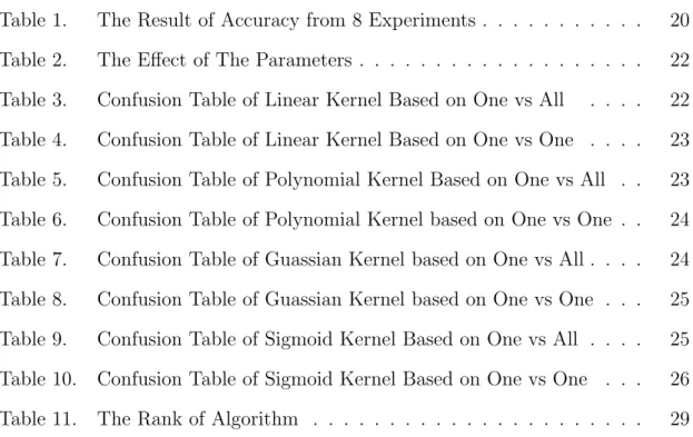
How to separate two different groups mathematically? Intuitively, we need to find the margin of each group, then draw a line (hyperplane in high dimension) between two closed margins so that it can separate them clearly. It may occur in two cases. Case 1, the line could be a straight line. Case 2, the line has to be a curve. See Fig. 1 for an example. The goal is to find the function of line, which is the classifier we need.
(a) Linear (b) NonLinear
Figure 1: Two Different Cases in SVMs
Usually, there are several possible hyperplanes satisfied this requirement, see the illustration in Fig. 2. Hence, there is naturally a question: which classifier is the best? We will give the answer in the next chapter.
2.1
Support Vector Machine
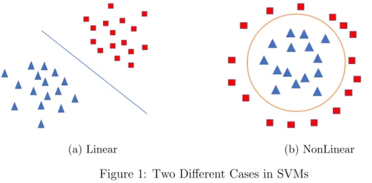
Support Vector Machines can find the best option to separate two different groups by maximizing the margin between the separating hyperplane. The function of hyperplane, which is called as the classifier, is usually specified by a small subset of training set, which are the support vectors. See Figure 3.
Figure 3: Key Ideas in SVMs
In this thesis, we assume all the training sample come from a determined distribution D. We also assume that there exists a knownBoolean value corre-sponding to each sample [6], e.g, {x1, x2, x3, ..., xn, y}, denoted as (x,y). Here, xi represents the feature of the sample,n is the number of the features, y is the Booleanvalue T rue(1) or F lase(−1), x and y are vector notations. As such, the units of a group will have a same label, which is the label of the group as well. We don’t have any special requirements for the distribution of x and y, which is differ-ent from with LDA. To make our theory easier to accept, we assume the training sample can be separated linearly for now.
2.2
Linear SVM
Linear model is the basis of SVM. Thus, we start with the linear model and explore the idea behind SVM.
Support Vector
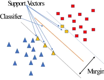
Figure 3 shows that the Support Vectors are the data sample lie on (or closed to)1 the boundary. Here, we can define support vector as the elements of the
train-ing set that would change the position of the optimal hyperplane if removed, which are the critical elements on training set [7]. Be careful, not every support vector will affect the hyperplane if it is removed. But the other points that are not sup-port vectors will definitely not affect the hyperplane at all even if they are removed.
In Figure 4a, we can clearly see that the hyperplane won’t change at all when square p is removed. But the hyperplanem will rotate to m0, and the bound-ary b1 and b2 will follow to b01 and b
0
2 when the square q is removed in Figure 4b.
This illustration explains and proves the definition. On the other hand, non-support vectors don’t contribute to the classifier is obviously true from Figure 4.
(a) No Effect (b) Effect
Figure 4: The effect of removing support vector
1Sometimes the data sample not exactly on but very close to the boundary, and they are also counted as Support Vectors. It will be use in the experiment.
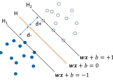
Hyperplane
Now, we define the hyperplane H such that wxi +b >+1, when yi = +1 wxi +b 6−1, whenyi =−1 (2.1)
As Figure 5 shows, H1 and H2 are the planes
H1 :wxi+b=−1, (2.2)
and
H2 :wxi+b= +1. (2.3)
H is the classifier:
wxi+b= 0. (2.4)
In these equations,xi is a data point, w is the coefficients of xi. Both xi and w
are vectors, and b is a constant.
Distance
Figure 5 is a projection from the high dimension space. H1, H2 and H are
the hyperplanes, the solid and empty dots stand for the sampling units. That’s why the different sampling units have the same label value (−1 or +1) even they are in distinct locations. From Figure 5, we can tell the points on the plane H1 and H2
are the support vectors from the previous definition. The points below or on the plane H1 are considered as one group. Similarly, we regard the points above or on
the plane H2 as another group. d represents the width of the margin, which is
ex-pected to be as big as possible, since in this case, H will separate two groups more clearly. To make it fair for both groups, we thinkH is in the middle of margin area and parallel to the boundaries.
It is well known that the distance from a point(x0,y0) to a line Ax+By+c=
0 is
d= |Ax√0+By0+c|
A2+B2 . (2.5)
Thus, the distance between the support vectors on H1 and H0 is
d= |wx√ +b|
w2 (2.6)
Since the points on plane H1 satisfywx+b =−1, and √ w2 =||w||, then d= | −1| ||w|| = 1 ||w|| (2.7)
Thus, the width of the margin is ||w2||.
Optimization
As we stated in the beginning of chapter, our goal is to maximize the width of the margin, equivalently, minimizing ||w||such that the discriminant boundary is
obeyed. Notice that the equation (2.1) could combine into a simpler form:
yi(wxi+b)>1 ∀i= 1,2,3, ..., n (2.8)
Minimizing ||w||is the same as
min 1 2||w||
2 (2.9)
As such, the problem is converted to solve the minimization problem in (2.9) with the constrained inequality in (2.8). Since polynomial (2.9) is quadratic with positive coefficients, there exist a minimum.
According to Karush–Kuhn–T uckerconditions(KT T) [8], the solution of problem 2.9 will be the saddle point of
Lp = 1 2||w|| 2− n X i=1 αi[yi(wxi+b)−1]. (2.10)
Here, αi is a nonnegative constant correspond to the nonnegative Lagrange
multi-plier1. However, we don’t like α too big as to make one vector has too much weight,
we say it is less than a positive constant c. Since this is a convex function, the min-imal point is the saddle point. At the this point, we take the partial derivative with respect to w, b and αi, then we have
∂Lp ∂w =w− n X i=1 αiyixi = 0, (2.11) ∂Lp ∂b =− n X i=1 αiyi = 0, (2.12) ∂Lp ∂αi =yi(wxi+b)−1 = 0 ∀i= 1,2, ..., n. (2.13)
From equation 2.13, we can conclude that the sampling units must be on the hyper-plane H1 or H2 when LP has the minimal. Also, we can get from equation 2.11 and
2.12 w = n X i=1 αiyixi n X i=1 αiyi = 0 (2.14)
Next, we substitute equation (2.14) into 2.9 and get
min Lp = 1 2 n X i=1 n X j=1 αiαjyiyjxixj− n X i=1 αiyi(xi n X j=1 αjyjxj +b) + n X i=1 αi = 1 2 n X i=1 n X j=1 αiαjyiyjxixj− n X i=1 n X j=1 αiαjyiyjxixj −b n X i=1 αiyi+ n X i=1 αi =−1 2 n X i=1 n X j=1 αiαjyiyjxixj+ n X i=1 αi s.t. αi >0 ∀ i= 1,2, ..., n. (2.15)
Equivalently, the above minimum can be substituted by
max LD(αi) = n X i=1 αi− 1 2 n X i=1 n X j=1 αiαjyiyjxixj (2.16) s.t. n X i=1 αiyi = 0 and c>αi >0 ∀i= 1,2, ..., n. (2.17)
Notice that we have removed the dependence from w and b intoαi. After we find
every αi, we can get w from the equation 2.14, b from 2.13 with the limitationc > αi >0.
The maximal of Eq. (2.16) can be easily found by the quadratic program-ming. Of course, we don’t want to do this problem by hand, since there are tons of simulations, manipulations and iterations. This procedure can be done by the pack-age CVXOPT2 in Python.
2CVXOPT is a free software package for convex optimization based on the Python program-ming language.
After we get w∗ and b∗, the function of classifier will become
Boolean=sign(w∗x+b∗) (2.18)
How to use this classifier when we have a unlabeled test sample unit? First, plug in the unit into equation 2.18. Then, the output of the function is ”-1” or ”1”. Recall the beginning of the chapter, we mentioned each group have a unique
Booleanvalue as the label. Then this unit will belong to the group which has the same label.
2.3
Non Linear SVMs
However, the assumption that two groups are linearly separable is not al-ways true in real life. How can we deal with those cases? This section will give the solution. Still, we are going to start with two dimensional cases then generalize the conclusion to the high dimensional space.
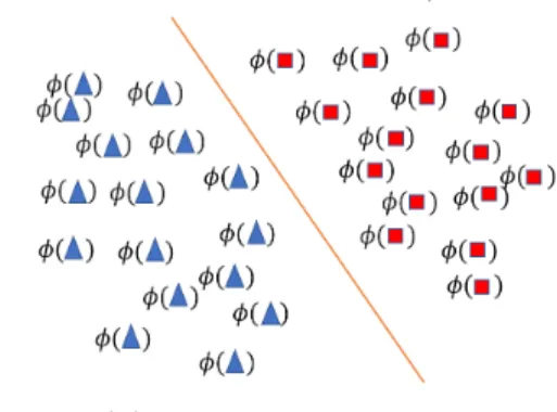
Transformation
In this section, the key ideal is the data transformation. In Figure 6a, even though the boundary is not linear, we can use some functionφ(xi) so that inputting
the original data sample will output the linearly separable data set as Figure 6b.
(a) Before Transformation (b) After Transformation
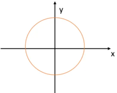
So, what’s the function of φ(xi) then? Particularly, we can set the
hyper-plane in a X-Y coordinate system in Figure 7, X and Y are the data features. Then, we obtain
Figure 7: The hyperplane of Figure 6a
There are 4 intersection point between the separating line and X-axis. So, we can assume
x2 = (x1−r1)(x1 −r2)(x1−r3)(x1−r4) (2.19)
Here, r1, r2, r3, r4 are the roots of φ(x1).
Recall the Figure 1b, we can have the separating hyperplane as Figure 8.
Figure 8: The hyperplane of Figure 1b
Since the hyperplane is a circle, more general, we can consider it as an el-lipse. So, we can assume
1 = r x2 1 a2 + x2 2 b2 (2.20)
Optimization
Recall, the Lagrange Function 2.10 where xixj is the dot product of two feature vectors. Since we transfer the feature vector x toφ(x), we need to substi-tute xixj toφ(xi)φ(xj) as well, which is a function of xi and xj. There exists a “kernel function” K [9] such that K(xi,xj) =φ(xi)φ(xj).
There are three popular kernel functions used in SVMs as the following. First, polynomial Kernel:
K(xi,xj) = (xTi xj+ 1)p (2.21)
Second,radial-basis Kernel:
K(xi,xj) = exp −||xi−xj|| 2σ2 (2.22)
Third, SigmoidKernel:
K(xi,xj) = tanh β0xiTxj +β1
(2.23)
Here, T stands for the transpose of a vector, p,σ, β0 and β1 are all user defined
parameters. We can adjust the parameters in order to get a better result during the actual experiment. In particularly, the function 2.21 is associated with equation 2.19 and the function 2.22 is correspond to 2.20.
Follow the procedure like what we did in the linear case, we just substitute
x toφ(x), then we will get the similar Lagrangian function:
Lp = 1 2||w|| 2− n X i=1 αi[yi(wφ(xi) +b)−1]. (2.24)
multi-plier and less than a positive constant c. Since this is a convex function, the mini-mal point is the saddle point. At the this point, we take the partial derivative with respect to w, b and αi, yielding
∂Lp ∂w =w− n X i=1 αiyiφ(xi) = 0, (2.25) ∂Lp ∂b =− n X i=1 αiyi = 0, (2.26) ∂Lp ∂αi =yi(wφ(xi) +b)−1 = 0 ∀i= 1,2, ..., n. (2.27)
From equation 2.27, we can easily conclude that the sampling units must be on the hyperplane H1 orH2 when LP has the minimal. We can get from equation 2.25 and
2.26 that w = n X i=1 αiyiφ(xi) n X i=1 αiyi = 0 (2.28)
Next, we substitute equation 2.14 into 2.9 and get
minLp = 1 2 n X i=1 n X j=1 αiαjyiyjφ(xi)φ(xj)− n X i=1 αiyi(φ(xi) n X j=1 αjyj(φ(xj) +b) + n X i=1 αi = 1 2 n X i=1 n X j=1 αiαjyiyjφ(xi)φ(xj)− n X i=1 n X j=1 αiαjyiyjφ(xi)φ(xj)−bn n X i=1 αiyi+ n X i=1 αi = 1 2 n X i=1 n X j=1 αiαjyiyjK(xi,xj)− n X i=1 n X j=1 αiαjyiyjK(xi,xj) + n X i=1 αi =−1 2 n X i=1 n X j=1 αiαjyiyjK(xi,xj) + n X i=1 αi s.t. c >αi >0 ∀i= 1,2, ..., n
Equivalently, the above minimization problem can be rewritten as
max LD(αi) = n X i=1 αi− 1 2 n X i=1 n X j=1 αiαjyiyjK(xi,xj) (2.29)
s.t. n
X
i=1
αiyi = 0 and c>αi >0 ∀i= 1,2, ..., n
So, the non linear SVMs is similar to linear SVM, and the only difference is that nonlinear SVM uses different kernel functions rather than the original inner product xixj. Hence, we can still find everyαi by the CVXOPT package.
As equation 2.18 shows, we can determine the label of the testing unit z in a way similar to linear SVM. First of all, we need transform (z) to φ(z), then the classifier would be Boolean=sign(w∗φ(z) +b∗) (2.30) =sign( n X i=1 αiyiφ(xi)φ(z) +b∗) (2.31) =sign( n X i=1 αiyiK(xi,z) +b∗) (2.32)
After we have theboolean value, the same determination will be applied here with the linear case.
3. EXPERIMENTAL DESIGN
In this chapter, we are going to apply the technology we have introduced in the last chapter into a real world problem, handwritten digital recognition. The theory of last chapter can only apply for two-classes recognition, but the digital recognition is a matter of ten classes. Hence we have to divide this multi-classes problem into several two-classes cases, then solve them by some inner algorithm. Two main technologies will be demonstrated in the following, they are similar in the ideal but different in the performance.
3.1
Sample Space
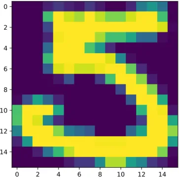
First of all, we need to learn the property of the data in order to get a bet-ter result. The sample comes from the zip code on the envelopes3, separated into
two subsets, training set and testing set. All of them have been converted from the image with dimension 16*16 pixel as Figure 9 shows into a min-max normalization[10] vector with its label as the first element of this vector. e.g.
[5.,−1.,−1.,−1.,−0.813, ...,−0.671,−0.095,−0.671,−0.828,−1.]
Here,“5” means that this vector is the representation of digit 5, all the numbers behind are the gray-scale values of a pixel after min-max normalization, which have the minimum 0 and maximum 255 so that we can apply this normalized technology here. In addition, “0” corresponds to all black color and “255” stands for all white color. That’s why the length of this vector is 257 = 1 + 16×16.
Secondly, how to use this sample space? As the name suggests, the training sample is for the purpose of training algorithm and find the classifiers. And testing
3These data were kindly made available by the neural network group at AT&T research labs (thanks to Yann Le Cunn).
0 2 4 6 8 10 12 14 0 2 4 6 8 10 12 14
Figure 9: One of Sample Unit
sample is for testing if our classifiers are sufficient and how well it perform. Usually, the training sample has the bigger size than the testing one. In our case, they have 7291 and 2007 sample units, respectively.
3.2
One v.s. All
As two technologies we mentioned at the beginning of this chapter, let’s start with an easier, common and more acceptable one, One v.s. All. Here are the following steps to establish this whole process:
Step 1: Classify the sampling units by their labels into 10 subsets; Step 2: Randomly4 select 100 sample units from each subset;
units with label “0” and reset the label as “+1”; another one (not 0) is the combination of 100 sample units from the rest of subsets and reset the label of combination as “-1”;
Step 4: Run the Linear SVMs algorithm with two classes from step 3 and get the pa-rameterw0 and b0;
Step 5: Make the second two-classes recognition, one class is the subset including all the units with label “1” and reset the label as “+1”; another one (not 1) is the combination of 100 sample units from the rest of subsets and reset the label of combination as “-1”;
Step 6: Run the Linear SVMs algorithm between two classes from the last step and get the parameterw1 and b1;
Step 7: Similarly, run the last two step for “2” and “not 2”, “3” and “not 3”,...,“9” and “not 9”, and get w2 and b2, ..., w9 and b9
Step 8: Obtain 10 classifiers if the testing unit is x,
y0 =w0x+b0 (3.33)
y1 =w1x+b1 (3.34)
..
. ... ... (3.35)
y9 =w9x+b9 (3.36)
Step 9: Plug in a testing sample unit into the 10 classifiers, we will get one output from each one;
Step 10: Compare among all 10 outputs and find the maximum of them. Then the testing unit will belong to the group with the label with the subscript of the classifier who give the largest output;
Step 11: Change Linear SVMs into Non Linear SVMs with three different kernel func-tion and run the same algorithm three times;
Step 12: Summarize the accuracy of recognizing of each digit from each algorithm.
The above steps complete the One v.s. All process of SVMs. Noboby knows if the two-classes are linearly separable specially when they are in high dimensional space, so we will try them all and find the better one. In addition, the above ex-periment involved some parameters need to be specified by the designer ahead. As such, some experience may required when we adjust the parameters.
3.3
One v.s One
One v.s One technology will involve another two mathematical tricks, com-binatorics and voting. Before we go to the main topic, let’s get familiar with them first. The number of ways we can chose two objects from 10 is 102 = 10(102−1) = 45, this is the combinatorics we need to use later.
Assume there are 10 wrestlers in the battlefield and there is a fight between every two of them, only win or lose, not tie. There are 45 fights in total. How can we decide which one the best most likely is after all the fights done? A reasonable rule is called voting process, that is, a wrestler will earn one point if he wins, and his points will not be deducted if he loses and the points can be accumulated; fi-nally, the wrestler who accumulates the most points will be the best.
After introducing those two definition, we are ready to design the process of One v.s One, which is sketched as below
Step 1: Classify the sampling units by their labels into 10 subsets;
Step 3: Pick two of them from 10 new subsets, note Φi and Φj.Here i and j are the
original labels of two subsets. Reset the label of Φi as “+1” and Φj’s as “-1”;
Step 4: Run linear SVMs algorithm using Φi and Φj, get the parameters wij and bij;
Step 5: Repeat the last two step for any two of subsets without the duplication. Step 6: Obtain 45 classifiers if the testing unit is z, then
yij =wijz+bij i < j ∈ {0,1, ...,9} (3.37)
Step 7: We will get one output from every classifier and record them;
Step 8: Run the voting process for the testing sample unit by counting “+1” as the subset Φi win and “-1” as the subset Φi lose;
Step 9: Counting the score for each subset, then the unit will belong to the subset who has the biggest score;
Step 10: Change linear SVMs into nonlinear SVMs with three different kernel functions and run the same algorithm three times;
Step 11: Summarize the accuracy of recognizing of each digit from each algorithm. The above steps complete the One v.s. One process of SVMs. Even though it has shorter steps than the process of One v.s. All, it has much more computation than the latter. During the manipulation, finding the classifier spends most of time. Obviously, this process need 102 classifiers but the last one only need 10, and this difference will become more distinguishable if there are more classes. Moreover, the voting processing takes longer than finding the maximum. Hopefully, this process can give us the better result to make our extra work paid off.
4. EXPERIMENTAL RESULT
This chapter verifies our theory and the experimental design. The results are obtained from a laptop computer with Window 10 64-bit operating system, 8.00GB RAM with the processor Inter(R) Core(TM) i7-6500U CPU @2.50GHz 2.6GHz, x64-based. We will do comparisons between linear and nonlinear models, with One v.s. One and One v.s. All strategies.
4.1
Accuracy
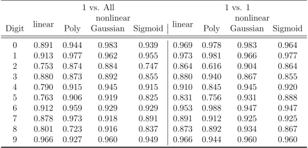
Table 1 gives the accuracy result from 8 different experimental designs. It shows the results from the two strategies that were stated in the last chapter, One vs One and One vs All. Each course separated as two sections, linear and nonlin-ear. Particularly, nonlinear section has three cases stand for its own kernel func-tions, polynomial, Gaussian and sigmoid.
Table 1: The Result of Accuracy from 8 Experiments
1 vs. All 1 vs. 1
linear nonlinear linear nonlinear
Digit Poly Gaussian Sigmoid Poly Gaussian Sigmoid
0 0.891 0.944 0.983 0.939 0.969 0.978 0.983 0.964 1 0.913 0.977 0.962 0.955 0.973 0.981 0.966 0.977 2 0.753 0.874 0.884 0.747 0.864 0.616 0.904 0.864 3 0.880 0.873 0.892 0.855 0.880 0.940 0.867 0.855 4 0.790 0.915 0.945 0.915 0.910 0.845 0.945 0.920 5 0.763 0.906 0.919 0.825 0.831 0.756 0.931 0.888 6 0.912 0.959 0.929 0.929 0.953 0.988 0.947 0.947 7 0.878 0.973 0.918 0.891 0.891 0.912 0.925 0.925 8 0.801 0.723 0.916 0.837 0.873 0.892 0.934 0.867 9 0.966 0.927 0.960 0.949 0.966 0.944 0.960 0.960
The above Table represents the percentage of algorithm recognized the cor-rect digit from the testing sample. The first column are from 0 to 9, which are the
racy of 89.1% when it is recognizing the digits 0 in One vs All design with the nor-mal linear kernel. Hence, a bigger value implies better classification performance.
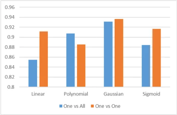
In general, the algorithm has a relatively good average accuracy on most of experiments as what the following Figure 10 shows. Most of them are around 90%, which is decent. Since this is handwritten digits not a printed body, even the hu-man will get confused on certain curves, it is acceptable. However, the polynomial kernel gave a weak result on One vs One design.
Figure 10: The Average Accuracy on Each Experiment
The above result are based on some specific parameters, which play a crucial role in this experiment. On certain ones, some accuracy are even 0. Table 2 shows the difference base on Gaussian kernel inOne vs All design.
From Table 2, we notice that there are huge difference in accuracy between case 1 and 3 even though they just have a slight different in σ. In case 2 and 3, there is a little difference on accuracy since the different is minor. Hence, the pa-rameters did effect the results a lot, but the variation may more or less. Therefore, this experiment does require the some experience to adjust the parameters.
Table 2: The Effect of The Parameters The Effect of the Parameters
Parameters Accuracy σ 0 1 2 3 4 5 6 7 8 9 case 1 1.0E-07 1 1.00 0.71 0.00 0.00 0.00 0.00 0.00 0.00 0.00 0.00 case 2 1.0E-05 10 0.99 0.97 0.87 0.87 0.94 0.91 0.95 0.92 0.90 0.95 case 3 1.0E-07 10 0.98 0.96 0.88 0.89 0.95 0.92 0.93 0.92 0.92 0.96
4.2
Confusion Table
In this section, we are going to look inside to find what mistake the algo-rithm made and if they are reasonable. By given Table 3 to 10, which are the con-fusion matrices of each algorithm, it will be much more easier to investigate what decision the algorithm had made in detail.
Table 3: Confusion Table of Linear Kernel Based on One vs All Output Digits 0 1 2 3 4 5 6 7 8 9 Actual Digits 0 320 0 3 7 4 2 13 0 7 3 1 0 241 1 2 8 0 4 1 2 5 2 2 0 149 10 14 1 3 2 14 3 3 1 0 3 146 0 6 1 2 3 4 4 0 1 3 0 158 0 5 2 4 27 5 2 0 1 14 4 122 3 1 7 6 6 2 0 5 0 4 2 155 0 2 0 7 0 0 0 2 8 0 0 129 0 8 8 2 0 4 5 5 7 4 2 133 4 9 0 0 0 0 3 0 0 2 1 171
Table 4: Confusion Table of Linear Kernel Based on One vs One Output Digits 0 1 2 3 4 5 6 7 8 9 Actual Digits 0 348 0 1 0 3 0 5 1 1 0 1 0 257 1 2 1 0 3 0 0 0 2 4 1 171 6 4 2 3 3 4 0 3 4 0 2 146 0 8 0 1 4 1 4 1 3 5 0 182 1 2 1 1 4 5 4 0 1 12 2 133 2 0 2 4 6 0 0 2 0 2 2 162 0 2 0 7 1 0 1 0 6 0 0 131 0 8 8 4 0 2 3 4 7 0 1 145 0 9 0 0 0 0 3 1 0 2 0 171
Table 5: Confusion Table of Polynomial Kernel Based on One vs All Output Digits 0 1 2 3 4 5 6 7 8 9 Actual Digits 0 339 3 1 0 3 1 5 6 0 1 1 0 258 0 1 2 0 2 1 0 0 2 0 2 173 5 3 0 1 13 1 0 3 0 0 1 145 0 12 0 6 0 2 4 0 4 2 0 183 1 1 5 0 4 5 1 1 0 3 1 145 0 5 0 4 6 0 1 1 0 4 1 163 0 0 0 7 0 0 0 0 4 0 0 143 0 0 8 2 5 3 8 3 5 3 17 120 0 9 0 2 0 0 1 0 0 10 0 164
Table 6: Confusion Table of Polynomial Kernel based on One vs One Output Digits 0 1 2 3 4 5 6 7 8 9 Actual Digits 0 342 12 1 0 0 0 2 2 0 0 1 0 261 0 0 3 0 0 0 0 0 2 4 107 75 2 2 0 1 5 2 0 3 2 25 0 137 0 1 0 0 0 1 4 0 40 0 0 157 0 1 1 0 1 5 4 79 0 19 1 53 0 3 0 1 6 1 35 1 0 2 0 131 0 0 0 7 0 12 1 0 3 0 0 131 0 0 8 3 35 0 6 2 2 0 10 108 0 9 0 12 0 0 2 1 0 17 0 145
Table 7: Confusion Table of Guassian Kernel based on One vs All Output Digits 0 1 2 3 4 5 6 7 8 9 Actual Digits 0 353 0 2 0 3 0 0 0 0 1 1 0 254 0 2 3 0 3 1 1 0 2 3 0 175 3 8 1 1 1 6 0 3 2 0 4 148 0 7 0 0 4 1 4 0 2 3 0 189 0 1 1 0 4 5 3 0 0 4 1 147 0 0 1 4 6 3 0 3 0 3 2 158 0 1 0 7 0 0 2 0 6 0 0 135 1 3 8 2 0 2 5 1 3 0 0 152 1 9 0 0 0 0 3 1 0 1 2 170
Table 8: Confusion Table of Guassian Kernel based on One vs One Output Digits 0 1 2 3 4 5 6 7 8 9 Actual Digits 0 353 0 2 0 2 0 0 0 2 0 1 0 255 0 1 3 0 4 0 0 1 2 2 0 179 3 5 2 0 1 6 0 3 1 0 4 144 0 11 0 0 5 1 4 0 1 3 0 189 1 1 1 1 3 5 3 0 0 3 1 149 0 0 1 3 6 0 0 3 0 2 3 161 0 1 0 7 0 0 1 0 6 1 0 136 1 2 8 2 0 0 1 0 4 1 1 155 2 9 0 0 0 1 4 0 0 0 2 170
Table 9: Confusion Table of Sigmoid Kernel Based on One vs All Output Digits 0 1 2 3 4 5 6 7 8 9 Actual Digits 0 337 0 3 2 3 1 7 1 3 2 1 0 252 1 2 3 0 3 0 1 2 2 3 0 148 5 20 2 3 2 14 1 3 1 0 3 142 1 12 0 2 1 4 4 0 1 1 0 183 0 5 1 1 8 5 5 0 0 10 5 132 1 0 2 5 6 1 0 2 1 4 3 158 0 1 0 7 0 0 1 0 6 0 0 131 1 8 8 3 0 1 5 4 4 2 4 139 4 9 0 0 0 0 4 1 0 2 2 168
Table 10: Confusion Table of Sigmoid Kernel Based on One vs One Output Digits 0 1 2 3 4 5 6 7 8 9 Actual Digits 0 346 0 1 0 3 0 6 1 2 0 1 0 258 0 1 2 0 3 0 0 0 2 5 0 171 6 6 1 3 1 4 1 3 2 0 2 142 1 14 0 1 3 1 4 0 3 3 0 184 0 3 1 1 5 5 4 0 0 8 2 142 0 0 0 4 6 0 0 3 0 3 3 161 0 0 0 7 0 1 0 1 6 0 0 136 1 2 8 4 0 0 3 4 7 0 2 144 2 9 0 0 0 1 4 0 0 2 0 170
The above 8 Tables demonstrate the actually recognized result from each experiment. Every one has 10 rows and 10 columns. Since the testing sample units have its own label, we separate them digit by digit. For example, there are
320 + 0 + 3 + 7 + 4 + 2 + 13 + 0 + 7 + 3 = 359 (4.38)
testing units with label “0” in our test sample and the algorithm did correctly rec-ognize 320 of them, and recrec-ognized 3 of them as digit “2”, 7 of them as digit “3”, etc. So, the accuracy that the algorithm with Linear Kernel based on One vs All design is
320
359 = 0.891, (4.39)
which is consistent with the first element upper right on table 1.
Similarly, each digit from Table 3 to Table 10 has the same meaning. These tables are very important for improving the accuracy, they suggest the possible trend of error for each algorithm. Then, we can develop the suitable modification individually by these reference in order to increase the performance of the algo-rithms.
4.3
Time
As we all know, the sufficiency of one experiment is not only about the out-come, but also the cost. The main issue is time on our design and it can be con-sidered as two parts, training and recognizing. Since the training part we can do ahead, it takes up a smaller weight. Here are the details in the following Figure 11.
Figure 11: The Time Spend on Training and Recognizing
From this figure, we can clearly see that the time spend on One vs. All de-sign is uniformly less than One vs One dede-sign, which makes sense because the One vs One has a lot more classifiers than One vs All design does. Furthermore, the process of recognizing needs to bring every unit of the training sample into the clas-sifiers in the second design. In fact, we would rather the algorithm spend time as less as possible even though we have the super power computer today. No one is willing to wait the outcome in a few hour after give some input. Thus, we prefer to use the linear kernel than other kernels, One vs All design than One vs One design from the aspect of time consuming.
5. DISCUSSION
In the last chapter, we have given the main result of our experiments, which proved our theory is durable and effective in real scenario. However, it is worth to discuss more in detail, in particular, what advantages and disadvantages of SVM, compared to other classification algorithms. if there is any disadvantage, what im-provement should we do to increase the performance of experiment in the future.
5.1
Conclusion
From Figure 10, we can clearly see that One vs One design performs better than One vs All in accuracy as what we expect except the polynomial kernel case, this is because the second design has much more classifiers involved and the voting process is more convincing than one ticket call.
The algorithm with Gaussian Kernel has the best result, no matter in which design. These two designs deliver slightly different results and both are greater than 93%. As for the algorithm with linear kernel, it doesn’t have the best result on ac-curacy but it is unbeatable at the speed of recognition. Hence, it is really difficult to conclude which one is the best overall.
However, we can make an evaluation system based on their ranks to help us out. The weight of each index will be specified ahead by the preference of experi-ment. If we don’t care time consuming but the accuracy, give the rank of accuracy heavier weight, vice versa. In our case, we set the weight of accuracy as 70%, time as 30%. Then we have the following Table 11.
Based on this evaluation, we would like the algorithm with Gaussian Kernel in One vs All design. In the future, this evaluation system still can be used, just change the weight of indexes.
Table 11: The Rank of Algorithm
Rank Performance
Average Accuracy Time Consuming Score Rank
Linear 1vsAll 8 1 5.9 6 Ploynomial 1vsAll 5 3 4.4 5 Gaussian 1vsAll 2 5 2.9 1 Sigmoid 1vsall 7 4 6.1 8 Linear 1vs1 4 2 3.4 3 Ploynomial 1vs1 6 6 6 7 Gaussian 1vs1 1 8 3.1 2 Sigmoid 1vs1 3 7 4.2 4 Weight 70% 30%
5.2
Advantage and Disadvantage
In general, the Support Vector Machine classifier has better result on accu-racy compared to Regression Analysis. Since the regression model is more based on the continuous variables but classification problem only has two values originally, it is a discrete case.
Also, SVMs doesn’t require any prior knowledge about the object we focused on, the algorithm will learn the features from the training data set. For this reason, the SVM model can be generalized very easily. For example, it could do face de-tection, image classification, bioinformatics, etc, as long as we have the correspond training sample. The new classifiers can be found in the same pattern, and what we need to do is just changing a few parameters.
However, there are shortcoming as well. SVMs is a typical supervised train-ing algorithm, we need adjust the parameters to get a better output as what we showed in Gaussian kernel on One vs All design, which means that the result we have may not be the best since the parameter is not the best fit.
In addition, SVMs cannot memorize the new coming data units. For exam-ple, there is a testing unit coming and it gave an incorrect classification. There is
nothing the experimenter can do to help it improve. In another word, it will still give the same wrong answer if the same unit comes to classify. Therefore, it cannot be self improved.
5.3
Future Work
Two main assignments are increasing the accuracy and decreasing the time consuming in the future. Firstly, recalling the experimental design, the ”Not” train-ing set is randomly selected to balance the number of elements in two subsets. Since it is random, there exist some variations on the selected training set which will make a different classifier. Thus, the accuracy will change somehow.
From this perspective, there is a maximum in the varied accuracy. So, we can run the algorithm as many time as possible and store the parameter every time. Then compare with the outcome, chose the selected set as the final training set which gives the best result. In this way, I believe we can increase the accuracy.
Secondly, from Figure 9 we notice there is no sufficient value located in four corners. So we can get rid of the gray values in the four corners, to reduce the di-mension of the vector and simply the manipulation and save the time eventually.
REFERENCES
[1] B. Sch¨olkopf and A. J. Smola, Learning with kernels: support vector machines,
regularization, optimization, and beyond. MIT press, 2002.
[2] C. L. Devasena, T. Sumathi, V. Gomathi, and M. Hemalatha, “Effectiveness evaluation of rule based classifiers for the classification of iris data set,”
Bon-fring International Journal of Man Machine Interface, vol. 1, p. 5, 2011.
[3] N. Zahir and H. Mahdi, “Snow depth estimation using time series passive mi-crowave imagery via genetically support vector regression (case study urmia lake basin),” The International Archives of Photogrammetry, Remote Sensing
and Spatial Information Sciences, vol. 40, no. 1, p. 555, 2015.
[4] Z. Ye, M. Wang, C. Wang, and H. Xu, “P2p traffic identification using support vector machine and cuckoo search algorithm combined with particle swarm optimization algorithm,” in Internet Conference of China. Springer, 2014, pp.
118–132.
[5] S. Suralkar, A. Karode, P. W. Pawade et al., “Texture image classification
us-ing support vector machine,” International Journal of Computer Applications
in Technology, vol. 3, no. 1, pp. 71–75, 2012.
[6] Z. Songfeng, L. Xiaofeng, Z. Nanning, and X. Weipu, “Unsupervised clustering based reduced support vector machines,” in Acoustics, Speech, and Signal
Pro-cessing, 2003. Proceedings.(ICASSP’03). 2003 IEEE International Conference
on, vol. 2. IEEE, 2003, pp. II–821.
[7] R. Berwick, “An idiot’s guide to support vector machines (svms),” Retrieved
[8] C.-C. Chang, C.-W. Hsu, and C.-J. Lin, “The analysis of decomposition meth-ods for support vector machines,” IEEE Transactions on Neural Networks,
vol. 11, no. 4, pp. 1003–1008, 2000.
[9] B. Sch¨olkopf, R. Herbrich, and A. J. Smola, “A generalized representer theo-rem,” in International conference on computational learning theory. Springer,
2001, pp. 416–426.
[10] Y. K. Jain and S. K. Bhandare, “Min max normalization based data pertur-bation method for privacy protection,”International Journal of Computer &