2009-01-2749
Air-to-Fuel and Dual-Fuel Ratio Control of an Internal Combustion Engine
Stephen Pace and Guoming G. Zhu
Michigan State University
ABSTRACT
Air-to-fuel (A/F) ratio is the mass ratio of the air-to-fuel mixture trapped inside a cylinder before combustion begins, and it affects engine emissions, fuel economy, and other performances. Using an A/F ratio and dual-fuel ratio control oriented engine model, a multi-input-multi-output (MIMO) sliding mode control scheme is used to simultaneously control the mass flow rate of both port fuel injection (PFI) and direct injection (DI) systems. The control target is to regulate the A/F ratio at a desired level (e.g., at stoichiometric) and fuel ratio (ratio of PFI fueling vs. total fueling) to any desired level between zero and one. A MIMO sliding mode controller was designed with guaranteed stability to drive the system A/F and fuel ratios to the desired target under various air flow disturbances. The performance of the sliding mode controller was compared with a baseline multi-loop PID (Proportional-Integral-Derivative) controller through simulations and showed improvements over the baseline controller. Finally, the engine model and proposed sliding mode controller are implemented into a Hardware-In-the-Loop (HIL) simulator and a target engine control module, and HIL simulation is conducted to validate the developed controller for potential implementation in an automotive engine.
INTRODUCTION
Increasing concerns about global climate changes and ever-increasing demands on fossil fuel capacity call for reduced emissions and improved fuel economy. Vehicles equipped with DI fuel systems have been introduced to markets globally. In order to improve DI engine full load performance at high speed, Toyota introduced an engine with a stoichiometric injection
system with two fuel injectors for each cylinder, see [1]. One is a DI injector generating a dual-fan-shaped spray with wide dispersion, while the other is a port injector. The dual-fuel system introduces one additional degree of freedom for engine combustion optimization to reduce emissions with improved fuel economy.
Using gasoline PFI and ethanol DI dual-fuel system to substantially increase gasoline engine efficiency is described in [2]. The main idea is to use a highly boosted small turbocharged engine to match the performance of a much larger engine. Direct injection of ethanol is used to suppress engine knock at high engine load due to its substantial air charge cooling resulting from its high heat of vaporization.
The control of A/F ratio is an increasingly important control problem due to federal and state emission regulations. Operating the spark ignited internal combustion engines at a desired A/F ratio is due to the fact that the highest conversion efficiency of a three-way catalyst occurs around stoichiometric A/F ratio.
There have been several fuel control strategies developed for internal combustion engines to improve the efficiency and to reduce exhaust emissions. A key development in the evolution was the introduction of a closed-loop fuel injection control algorithm [3], followed by a linear quadratic control method [4], and an optimal control and Kalman filtering design [5]. Specific applications of A/F ratio control based on observer measurements in the intake manifold were developed in 1991 [6]. Another approach was based on measurements of exhaust gases by an oxygen sensor and the throttle position [7]. Hedrick also developed a nonlinear sliding mode control of A/F ratio based upon the oxygen sensor feedback [8]. The conventional A/F ratio control for automobiles uses both closed-loop Copyright © 2009 SAE International
feedback and feed forward control to achieve good steady state and transient responses.
The control strategies, mentioned above, were mainly for PFI systems. Mitsubishi began to investigate combustion control technologies for direct injection engines in 1996 [9]. Due to the introduction of internal combustion engines with dual-fuel systems (PFI and DI), control of both A/F ratio and fuel ratio (ratio of PFI fueling vs. total fueling) became part of a combustion optimization problem in [10].
In this paper, a control oriented model of a dual-fuel system is developed for control development and evaluation purposes, and a MIMO sliding model controller is developed to regulate the engine A/F and fuel ratios to target levels. The control strategy is validated in simulation based upon the developed dual-fuel system model. Furthermore, the engine model and proposed sliding mode controller are implemented into a Hardware-In-the-Loop (HIL) simulator and a target engine control module, and HIL simulation is conducted to validate the developed controller for potential implementation in an automotive engine
This paper is organized as follows. It begins by presenting a simplified A/F and fuel ratio control oriented model, followed by a section that describes an innovative sliding mode controller that regulates both A/F and fuel ratios to desired nonzero targets and simulation results are shown. Next, a state estimator will be presented for a fixed engine operation condition and the HIL environment setup will be described. Finally, HIL simulation results are presented and conclusions are discussed.
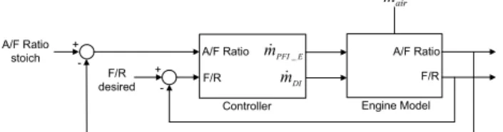
A/F RATIO AND FUEL RATIO ENGINE MODEL
The control problem of this work is to vary both fuel mass injection rates (mPFI and mDI) so that the engine A/F ratio is regulated at a desired level (e.g., stoichiometric) and the fuel ratio of effective PFI fueling,
E PFI
m _ , to total fueling, mtotal mPFI_EmDI, is maintained at a desired value as shown in Figure 1. Note that the effective fueling for DI is equal to the injected DI fuel.
A/F Ratio
stoich A/F Ratio
F/R Engine Model Controller F/R F/R desired E PFI m _ air m + -+ -A/F Ratio DI m
FIGURE 1: DIAGRAM OF A/F AND FUEL RATIO CONTROL PROBLEM
A nonlinear model for this problem, using simplified engine dynamics to model both the engine A/F and fuel ratios, is to be discussed below. The air flow, m air, is
model as Z Z Z 0' air m , (1)
where 0 is the nominal air flow and is the air flow disturbance due to the engine operational condition changes. The fuel flow for wall-wetting dynamics from the port fuel injector is modeled by the following transfer function , 1 1 ) ( ) ( _ s s s m s m PFI E PFI E D (2) where and are selected to be 0.5 and 0.8, respectively, in this model. The fuel flow from the direct injector contains negligible dynamics.
Due to the three-way catalyst used for emission control, most engines are design to achieve a target A/F ratio around stoichiometry. For this research, we use a normalized target A/F ratio, target, which is defined as
desired fuel ratio divided by stoichiometric air-to-fuel ratio (14.6 for gasoline). Note that at stoichiometry the normalized target A/F ratio is equal to one. The normalized A/F ratio can be expressed as:
. 6 . 14 total air m m O (3)
Now, the engine equivalence ratio I is defined as the inverse of relative A/F ratio and can be approximated using equations (1) and (3) below
¸¸¹ · ¨¨© § ' |
Z
Z
Z
I
2 0 0 1 1 6 . 14 mtotal , (4)where equation (1) is approximated by a first order Taylor expansion. For the rest of the paper, we consider only equivalence ratio control instead of A/F ratio. The fuel ratio of the dual-fuel system is defined as the effective PFI fueling divided by total fueling, where
total E PFI DI E PFI E PFI fuel m m m m m R _ _ _ . (5)
Similarly, fuel ratio, Rfuel, can be approximated by
substituting equation (4) into (5), replacing the engine equivalence ratio with the target ratio. Therefore,
et t E PFI fuel m R 2 arg 0 0 _ / 1 6 . 14 I Z Z Z ¸¸¹ · ¨¨© § ' (6)
The equivalence and fuel ratio model, operating at a fixed engine speed (1500RPM), includes wall-wetting dynamics of PFI fuel system, average DI fuel injection delay (50ms), oxygen (A/F ratio) sensor delay (40ms), and air flow travel delay from engine throttle to cylinder (200ms). These time delays are approximated by unitary gain first order transfer functions. The complete model is divided into three subsystems, as shown in Figure 2, where the oxygen sensor dynamics are denoted as G1, the air flow dynamics as G2, and the fuel flow dynamics as G3. The state space equations of the three subsystems are shown in equations (7), (8), and (9). 1 1 1 1 1 1 1 1 x C y u B x A x (7) T T T C C C u D x C y u B x A x ] [ , 3 31 32 3 3 3 3 3 3 3 3 3 3 (8)
2 2 2 2 2 2 2 x C y B x A x Z (9) Fuel Ratio 2 Equivalence Ratio 1 Oxygen Sensor Dynamics (G1) In 1 Out1 Gain 14 .6
Fuel Flow Dynamics (G3) In1 In2 Out1 Out2 14 .6
Air Flow Dynamics (G2) In 1 Out1 Target Eq . Ratio 4 Air 3 DI 2 PFI 1
FIGURE 2: EQUIVALENCE AND FUEL RATIO MODEL
The entire system can be expressed by the following state-space model 3 3 2 2 3 31 2 1 3 2 1 0 0 0 0 0 0 u B B x x C C B x A A A x » » » ¼ º « « « ¬ ª » » » ¼ º « « « ¬ ª » » » ¼ º « « « ¬ ª » » » ¼ º « « « ¬ ª Z (10)
and the output equations for the equivalence and fuel ratios using (10) can be approximated by
3 2 31 2 6 . 14 CC x x yEqRatio (11) et t FuelRatio C x C x u y 14.6 2 2( 32 3.625 1)/Iarg (12) The values for the matrices of the engine model are
; 25 ; 6 . 14 ; 25 1 1 1 B C A ; 5 ; 1 ; 5 2 2 2 B C A . 0 625 . 0 0 0 ; 46875 . 0 0 0 0 20 20 ; 0 1 1 0 0 625 . 0 ; 1.25 -0 0 0 20 -0 0.4688 0 20 -3 3 3 3 » ¼ º « ¬ ª » ¼ º « ¬ ª » » » ¼ º « « « ¬ ª » » » ¼ º « « « ¬ ª D C B A
The nonlinear state space engine model must be transformed into the regular form [11] below to apply sliding mode control.
K fa(K,z)G(K,z); (13) u z G z f z b(K, ) (K, ) , (14)
where the forcing term of equation (13), (,z), contains the disturbance input and fa(,z) contains the
nonlinear portion of (10). A change of variables, x T z»¼ º « ¬ ªK (15) transfers the original state vector,
>
@
T x x x x x x 1 2 31 32 33 (16)into the regular form coordinates, where the transformation matrix T is chosen such that
T x x x x 0.625 ] [ 1 2 31 33 K (17) T x x z [ 33 32] (18)
Thus, the original system (represented in the regular form) is shown in (19) and (20). It can be seen that the model contains two control inputs corresponding to PFI and DI fueling and one mass air flow disturbance input.
0 1 -0 ) , ( 0 0 1 25 . 11 0 0 20 -0 0 0 5 -0 0 0 25 -) , ( ) , ( 1 3 2 1 z z fa z h z K G K G K K K K K » » » ¼ º « « « ¬ ª » » » ¼ º « « « ¬ ª » » » ¼ º « « « ¬ ª » » » ¼ º « « « ¬ ª » » » ¼ º « « « ¬ ª (19) » ¼ º « ¬ ª » ¼ º « ¬ ª » ¼ º « ¬ ª » ¼ º « ¬ ª 2 1 ) , ( 2 1 1 0 0 1 20 -0 0 25 . 1 -u u z z z G z fb K (20) where ). 0.625 ( 1460 ) , ( z 2 3 z1 z2 hK K K
SLIDING MODE CONTROL STRATEGY
Existing sliding mode A/F ratio control applications in [12] and [13] utilized the binary nature of a HEGO (Heated Exhaust Gas Oxygen) sensor to reduce its oscillation resulting from the time delay by using a dynamic, one dimensional sliding surface.
In this paper, a two dimensional sliding surface is selected to control both equivalence and fuel ratios of the dual-fuel system. The sliding surface is defined as
), (K I z s (21)
where the control objective is to regulate “s” to zero by designing a feedback I() such that it stabilizes equation (19). Letting » ¼ º « ¬ ª » ¼ º « ¬ ª 3 1 1 2 1 -1.6 ) (K K KK I zz z (22)
results in the asymptotic stability at the origin for (19) and decouples the nonlinear dynamics contained in
fa(,z) from the remaining equation. Also, I() does not
contain the state 2 and removes it from having any affect on the system, which is significant because the state 2 contained the input disturbance, . Differentiation of the sliding surfaces yields
>
( , ) ( , )@
) , ( ) , ( z G z u f z z f z s a b K GK K I K K K K I w w w w (23) Selecting the control u to cancel the known terms of (23)v z G z f z f z G u 1(K, ) b(K, ) KI a(K, )» 1(K, ) ¼ º « ¬ ª w w (24)
where v is the control input to be defined. Thus, ), , ( z v s GK K I w w (25) and . 0 0 1 -0 1 -0 1 -0 0 6 . 1 ) , ( » » » ¼ º « « « ¬ ª » ¼ º « ¬ ª w w GK z K I (26) Therefore (25) becomes . v z s w w K K I (27)
The selected v needs to force s toward zero and using
V = s2/2 as a Lyapunov function candidate for (25) then . v s v s s s V d (28)
Selecting v as 0 some for , 1 where ), sgn( t ! s b b v E E (29) leads to s VdE (30)
and therefore guarantees asymptotic stability. The resulting control forces the system states onto the sliding surface in finite time and eventually brings these states on the sliding surface to zero.
To achieve the desired nonzero equivalence and fuel ratios, consider 0 3 3 2 2 1 1 0 0 0 0 ) ( K K K K K K K K K K K K ' » » » ¼ º « « « ¬ ª ' (31) 0 2 2 1 1 0 0 0 ) (z z zz zz z z z z » ' ¼ º « ¬ ª ' (32)
where and z go to zero, leading and z converging to the target states 0 and z0 as time goes to infinity since the sliding mode controller regulates the states 1, 3 ,z1, and z2 to the sliding manifold s = 0. Using these target states, 0 and z0 can bring the equivalence ratio and fuel ratio to any desired value. Using (31) and (32), (19) and (20) become
» » » ¼ º « « « ¬ ª » » » ¼ º « « « ¬ ª ' ' ' ' » » » ¼ º « « « ¬ ª » ¼ º « ¬ ª ' ' » » » ¼ º « « « ¬ ª » » » ¼ º « « « ¬ ª ' ' ' » » » ¼ º « « « ¬ ª ' 0 0 0 0 0 0 0 0 0 0 0 0 0 0 1 3 2 1 2 1 3 2 2 1 3 2 2 1 2 2 3 2 1 2 2 1 3 25 . 11 20 5 25 ) 625 . 0 ( 1460 0 1 -0 ) 625 . 0 ( 0 0 1460 0 25 . 11 -0 0 1460 -625 . 0 1460 -20 -0 0 0 5 -0 1460 -) 625 . ( 1460 -25 -z z z z z z z z z K K K K K G K K K K K K K K K K (33) » ¼ º « ¬ ª » ¼ º « ¬ ª » ¼ º « ¬ ª » ¼ º « ¬ ª » ¼ º « ¬ ª ' ' » ¼ º « ¬ ª 0 0 2 1 2 1 2 1 20 0 0 25 . 1 1 0 0 1 20 -0 0 25 . 1 -z z u u z z z (34)
To investigate the stability of the system with these new target states, I() from (22) is used and by substituting
I() into (33), the final system becomes
. 25 . 11 20 5 25 ) 625 . 0 ( 1460 0 1 -0 20 -0 6 . 1 25 . 11 0 5 -0 0 ) 625 . ( 1460 -25 -0 1 0 3 0 2 0 1 0 2 0 1 0 3 0 2 3 2 1 0 2 0 1 0 3 » » » ¼ º « « « ¬ ª » » » ¼ º « « « ¬ ª » » » ¼ º « « « ¬ ª ' ' ' » » » ¼ º « « « ¬ ª ' z z z z z K K K K K G K K K K K (35) » ¼ º « ¬ ª » ¼ º « ¬ ª » ¼ º « ¬ ª » ¼ º « ¬ ª » ¼ º « ¬ ª ' ' » ¼ º « ¬ ª ' 0 0 2 1 2 1 2 1 20 0 0 25 . 1 1 0 0 1 20 -0 0 25 . 1 -z z u u z z z (36)
It can be seen that the nonlinear term of equation of (33) is now eliminated, leaving a linear term with constant
matrices plus the forcing term, and equation (34) remains linear. For entire system stability analysis, the characteristic equation of the linear matrix A* is
) 20 )( 25 . 1 )( 20 )( 5 )( 25 ( ) det(OIA* O O O O O
with all eigenvalues in the left half plane, where
. 20 -0 0 0 0 0 1.25 -0 0 0 0 0 20 -0 6 . 1 25 11. -0 0 0 5 -0 0 0 0 ) 625 . ( 1460 -25 -* 0 0 0 1 2 3 » » » » » » ¼ º « « « « « « ¬ ª z z A K
Note that the target states 0 and z0 can be determined with the given input air disturbance and desired equivalence and fuel ratios. The following output equations are the result of coordinate transformation of (11) and (12) (using (15)). ) 625 . 0 ( 20 5 25 ~ 2 1 3 2 1 z z yEqRatio K K K (37) et t FuelRatio z u y 14.6 5 2(0.468751 0.625 1)/ arg ~ K I (38)
Consider the state equations (19) and (20) at steady state by setting derivative terms equal to zero, leading to
EqRatio y ~ 25 1 1 K (39) ) 1 ( 5 1 5 1 2 G Z K (40) 1 3 20 25 . 11 z K (41) 1 1 1.25z u (42) 2 2 20z u (43)
Using (38), (43), and (39), we have ) 25 . 1 625 . 0 46875 . 0 ( 5 6 . 14 ~ 2 arg 1 K It et FuelRatio y z (44) 1 3 2 1 2 14.6255 20 0.625z z K K K (45)
Therefore, the system steady-state states and z can be expressed as a function of the desired output ratios and input disturbance. The target states 0 and z0 can be obtained with given target ratios and disturbance. The zero target state sliding mode control strategy is modified such that the closed-loop system converges to the desired target states, see Figure 3.
PFI m 0 K 0 z air m DI m
Figure 3: Schematic diagram of sliding mode control strategy
To improve the performance of the sliding mode controller, the stabilizing function I() can be generalized as follows » ¼ º « ¬ ª ' ' ' ' ' 3 1 3 1 -1.6 ) ( K K K H K K I z , (46)
where is a positive constant. Substituting (46) into (19) yields, 0 0 25 . 11 -20 -0 6 . 1 25 . 11 -0 5 -0 0 0 25 -3 2 3 2 1 H K K K K K H K ' » » » ¼ º « « « ¬ ª ' » » » ¼ º « « « ¬ ª ' ' ' » » » ¼ º « « « ¬ ª ' d (47)
where d = 91.25. Equation (47) can be viewed as ) , ( K H K K ' ' ' A g (48) where, . 0 0 ) , ( , 25 . 11 -20 -0 6 . 1 25 . 11 -0 5 -0 0 0 25 -) ( 3 2 H K K H K H H ' » » » ¼ º « « « ¬ ª ' ' » » » ¼ º « « « ¬ ª d g A
It can been seen that A() is Hurwitz if > 0 and also . 0 0 2 2 2 2 3 2 K H H K K ' d ' » » » ¼ º « « « ¬ ª ' d d (49)
Let Q = I and define X() > 0 as the solution of the Lyapunov equation assuming > 0
. ) ( ) ( ) ( ) ( X X A Q AT H H H H
The maximum and minimum eigenvalues of X() are plotted as function of in Figure 4.
0 10 20 30 40 50 60 70 80 90 100 0 0.005 0.01 0.015 0.02 H > 0 0 10 20 30 40 50 60 70 80 90 100 0 0.05 0.1 0.15 0.2 H > 0 Omax of X(H) Omin of X(H)
Figure 4: Maximum and minimum eigenvalues of X()
Define the Lyapunov function V() = TX(),
leading to the following properties:
. ) ( 2 2 2 , ) ( -, )) ( ( ) ( )) ( ( 2 max 2 2 2 2 2 min 2 2 max 2 2 min K O K K K K O K K K K K H O K K H O ' ' d ' ' w w ' d ' ' ' ' w w ' d ' d ' X X X V Q Q A V X V X T T (50)
The derivative of V() satisfies
. )) ( ( 2 ) ( -) ( 0 0 2 )) ( ) ( ) ( ) ( ( ) ( 2 2 3 max 2 2 min 2 3 K K H H O K O K H K K H K H H H H K K ' ' ' d ' » » » ¼ º « « « ¬ ª' ' ' ' ' d X Q X d A X X A V T T T
Therefore the origin is exponentially stable if
. )) ( ( 2 1 or 0 ) ( 3 max H K O H K ' ' d X V (51)
The stability condition will hold assuming
J K K
K d
' 3 3 30
for all time, where is a positive constant, and can be restated as: J H O H X d )) ( ( 2 1 max (52)
Figure 4 shows that max(X()) = 0.1 for all > 0, thus J J J H 5 . 182 1 625 . 0 1460 1 . 0 2 1 1 . 0 2 1 d (53)
Equation (53) shows that if is small, then there exists an > 0 with guaranteed stability.
SIMULATION RESULTS
A MIMO PID controller was designed for comparison purposes to the MIMO sliding mode controller. This controller cascaded two PID controllers such that the first PID is used to control the equivalence ratio and the second PI is used to reduce the fuel ratio error, see Figure 5. The controller gains for both PID and PI controllers are shown in Table 1.
+ Eq. Ratio error PID Controller Kd1 Kp1 Ki1 Kd2 Kp2 Ki2 s 1 s 1 s s + + Kp1 Ki1 1s Fuel Ratio error x mPFI DI m PI Controller
Figure 5: Schematic diagram of PID controller
All controller gain parameters were tuned such that the response of the closed-loop system was stable and had as fast a response as possible. Simulations of the sliding mode controller under different air flow input disturbances were conducted and compared to the PID controller.
Table 1: PID and PI controller parameters
Kp1 = Kp2 0.000005 Kp 0.5
Ki1 = Ki2 0.3 Ki 5
Kp1 = Kp2 0.0207
The gain matrix in the sliding mode controller for each simulation was tuned such that the transient response was acceptable and it was selected as
. 7 . 1 6 . 1 » ¼ º « ¬ ª E (54)
A unitary target equivalence ratio and 60% (0.6) target fuel ratio were chosen for each simulation. Figure 6 shows the closed-loop response of the PID controller and sliding mode controller for Simulation #1. The simulation uses a constant input disturbance of 0.1 plus 5 percent noise, adding a step input of 0.15 to the constant disturbance at the 6th second. It also has a fuel ratio reduction from 0.6 to 0.4 at the 9th second, and
shows that the controller rejects the disturbance quickly. Figure 6 also shows the PFI and DI fuel control inputs for both PID and sliding mode controllers. It can be observed that the sliding mode controller provides quick fueling inputs of both PFI and DI systems, leading to better disturbance rejection and transient response over the PID responses. Table 2 summarizes the overshoot and settling time for both PID and sliding mode controllers.
Table 2: Comparison of controllers for Simulation #1
% Overshoot
(after 6th second) (after 9Settling Time th second) (after 12ethss second)
PID Sliding Mode PID Sliding Mode PID Sliding Mode
Eq. Ratio 5.19% 2.44% 1.6 sec < 0.5 sec .016 .0003
Fuel Ratio 2.30% 2.61% 3.29 sec 2.31 sec .033 .0003
5 6 7 8 9 10 11 12 13 0 0.5 1 time (seconds) E qui va le nc e R at io 5 6 7 8 9 10 11 12 13 0 0.5 1 time (seconds) Fu el R at io Sliding Mode PID Sliding Mode PID 5 6 7 8 9 10 11 12 13 0 0.05 0.1 time (seconds) Sli ding M od e F u el ing 5 6 7 8 9 10 11 12 13 0 0.05 0.1 time (seconds) PI D Fu el in g PFI DI PFI DI
Figure 6: Closed loop response of simulation #1
TABLE 3: COMPARISON OF CONTROLLERS FOR SIMULATION #2
% Overshoot
(after 6th second) Settling Time (after 9th second) (after 12ethss second)
PID Sliding Mode PID Sliding Mode PID Sliding Mode
Eq. Ratio .99% .05% 0.45 sec 1.29 sec .0018 .0007
Fuel Ratio 29% 2.27% 1.53 sec < 0.1 sec .0042 .0005
Figure 7 shows the closed-loop response of both PID and sliding mode controllers for Simulation #2. This simulation decreases the target equivalence ratio from 1 to 0.9 at the 6th second, and increases it back to unity at the 9th second. Again, the constant input disturbance
was 0.1 plus 5 percent noise. Figure 7 also displays both fueling inputs of PID and sliding mode controllers. Although the PID controller has a faster equivalence ratio response than the sliding mode one, it is under the penalty of the fuel ratio control accuracy (huge spike during the transition). On the other hand, the sliding mode controller provides smooth transitions for both equivalence and fuel ratios. Therefore, the sliding mode control responses are more favorable over the PID ones. Table 3 summarizes the overshoot and settling time for both PID and sliding mode controllers for Simulation #2. It is worth to noting 29% fuel ratio overshoot for the PID controller while the sliding mode controller only has 1%.
5 6 7 8 9 10 11 12 13 0 0.5 1 time (seconds) E qui va le nc e R at io 5 6 7 8 9 10 11 12 13 0 0.5 1 time (seconds) Fu el R at io Sliding Mode PID Sliding Mode PID 5 6 7 8 9 10 11 12 13 0 0.05 0.1 time (seconds) S lid in g M od e F u eli n g 5 6 7 8 9 10 11 12 13 0 0.05 0.1 time (seconds) PI D Fu el in g PFI DI PFI DI
STATE ESTIMATOR DESIGN
The sliding mode control strategy was implemented using state feedback, but this state information will not be available for closed loop control since in practice only some of the state variables are measurable. In some cases, even though they are measurable, high cost prohibits utilizing state feedback. Therefore, to implement the sliding mode control scheme, a state estimator must be designed to obtain state information in real-time from the available measurements. They are the equivalence and fuel ratio outputs, and the PFI and DI fueling inputs.
Consider the nonlinear system described in equations (10), (11), and (12). Since state x2 can be estimated from the mass air flow sensor signal Z equipped on the engine, assuming that x2 is known, the system can be rewritten as u x x x x » » » » ¼ º « « « « ¬ ª » » » » ¼ º « « « « ¬ ª 0 1 1 0 0 625 . 0 0 ~ 25 . 1 -0 0 0 0 0 2 -0 0 46875 . 0 20 -0 0 1460 1460 25 -~ 2 2 (55) u x x x x x y et t et t » ¼ º « ¬ ª » ¼ º « ¬ ª 0 / 2125 . 8 0 0 ~ / 21875 . 34 0 0 0 0 1460 1460 0 ~ arg 2 arg 2 2 2 I I (56)
where
~
x
>
x
1x
3x
4x
5@
T and note that the system is now linear. Thus a linear state estimator can be constructed as Du x C y y y L Bu x A x ˆ ˆ ) ˆ ~ ( ˆ ˆ (57) The matrix L is designed such that A+LC is stable. The estimated system can be rewritten as>
@
Du x C y y u L LD B x LC A x » ¼ º « ¬ ª ˆ ˆ ~ ˆ ) ( ˆThis estimator is known as the Luenberger observer [14] and the error between the actual state
~
x
(
t
)
and the estimated statex
ˆ
(
t
)
is given by>
~@
>
ˆ ~ ˆ@
. ) ( ˆ ) ( ~ ) ( x x LC Bu x A Bu x A t x t x t eSince the eigenvalues of A+LC are in the left half plane,
f o o xt e t t t x t e() ~( ) ˆ( ), ( ) 0as
For a fixed air flow disturbance of 0.1, the steady state value of x2 = 0.18 and using the linear system estimation equation (57), a linear state estimator can be designed with the following system parameter matrices:
, 0441 . 3 0 0 019 . 0 0761 . 0 019 . 0 0 1 » » » » ¼ º « « « « ¬ ª L , 25 . 1 -0 0 0 0 20 -0 0 46875 . 0 20 -0 0 2 . 248 8 . 262 25 -A » » » » ¼ º « « « « ¬ ª , 0 1 1 0 0 625 . 0 0 » » » » ¼ º « « « « ¬ ª B 0 0 0 6.1759375, 0 8 . 262 8 . 262 0 » ¼ º « ¬ ª C . 0 2125 . 8 0 0 » ¼ º « ¬ ª D
HIL SIMULATION SETUP
The A/F and fuel ratio engine model was implemented into an Opal-RT HIL system using MATLAB/Simulink. The engine model was running on the Opal-RT HIL simulator at a sample period of 1 millisecond. Similarly, the sliding mode controller, along with state estimator, was discretized with a five-millisecond sample period (T = 0.005) and implemented in Simulink. Due to discretization, communication, and computational delays (see Figure 10), the system responses oscillate. In the HIL simulation, the gain E defined in (54) was tuned for minimal settling time without oscillation. Figure 8 shows the responses of the equivalence and fuel ratios for different Evalues. It turns out that when EHIL = 0.4E, the
HIL simulation provides the best response for the discretized sliding mode controller.
14 15 16 17 18 19 20 21 0.96 0.98 1 1.02 time (seconds) Eq u iv al en ce R at io 14.5 15 15.5 16 16.5 17 0.2 0.3 0.4 0.5 0.6 time (seconds) Fu el R at io 0.2E 0.4E 0.6E 0.8E 1.0E
Figure 8: Response of ratios for different sampling periods
The discrete Simulink model was then implemented into a Mototron Engine Control Module (ECU) sampled every 5 milliseconds. The Opal-RT HIL simulator communicates with the Mototron ECU controller through the high speed controller-area network (CAN), where signals were sent and received with minimal delay. The HIL simulation scheme is shown in Figure 9.
Figure 9: HIL engine model and controller setup
The Opal-RT simulation step size of 1 millisecond was chosen in order to emulate a real-world continuous time engine. Similarly, the Mototron data sampling rate of 5 milliseconds was the controller updating speed used in many production engine control systems. The CAN communication between Opal-RT and Mototron had a time delay between the time when signals were sent from Mototron and the time when they were received by Opal-RT, and vice versa. This delay was less than 1 millisecond for our setup.
Figure 10: HIL timing scheme
HIL SIMULATION RESULTS
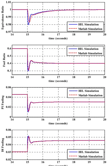
For the HIL simulation, a fixed air flow disturbance, , of 0.1 was used throughout the entire simulation. A unitary target equivalence ratio and 60% (0.6) target fuel ratio were chosen to begin the simulation. The equivalence ratio and fuel ratio responses of both HIL simulation and pure simulation are shown in Figure 11, which shows a fuel ratio reduction from 0.6 to 0.4 at the 15th second. Figure 11 also shows the PFI and DI fuel control inputs for both simulation environments. It can be observed that the HIL simulation responses is slightly slower than the pure simulation, which is due to both the feedback and control time delays between the HIL simulator and engine controller.
Figure 12 shows an equivalence ratio increase from
unity to 1.1 at the 40th second and also the
corresponding fueling inputs. Again the HIL simulation has a slower response than the pure simulation. For both the fuel ratio reduction and the equivalence ratio increase, the real-time sliding mode controller in the HIL environment was able to achieve the desired ratio values very well.
14 15 16 17 18 19 20 0.97 0.98 0.99 1 1.01 time (seconds) E q u iv al en ce R at io 14 15 16 17 18 19 20 0.3 0.4 0.5 0.6 time (seconds) Fu el R at io HIL Simulation Matlab Simulation HIL Simulation Matlab Simulation 14 15 16 17 18 19 20 0 0.02 0.04 0.06 time (seconds) PI Fu el in g 14 15 16 17 18 19 20 0.02 0.03 0.04 0.05 0.06 time (seconds) DI F u el in g HIL Simulation Matlab Simulation HIL Simulation Matlab Simulation Figure 11: Closed-loop response of HIL for fuel ratio reduction
CONCLUSION
A multi-input-multi-output sliding mode controller was developed based upon the A/F and fuel ratio model to achieve nonzero desired equivalence and fuel ratio target. The sliding mode controller was validated with the developed simple nonlinear dual-fuel system model and compared to the multi-loop PID controller. Furthermore, the controller was implemented in a real-time Hardware-In-the-Loop (HIL) environment and the results show that it is feasible to be implemented in a production engine control module controller.
39 40 41 42 43 44 45 46 1 1.05 1.1 time (seconds) E qui va le nc e R ati o 39 40 41 42 43 44 45 46 0.5 0.55 0.6 0.65 time (seconds) Fu el R at io HIL Simulation Matlab Simulation HIL Simulation Matlab Simulation 39 40 41 42 43 44 45 46 0.04 0.05 0.06 time (seconds) PI Fu el in g 39 40 41 42 43 44 45 46 0.02 0.025 0.03 0.035 0.04 time (seconds) DI F u el in g HIL Simulation Matlab Simulation HIL Simulation Matlab Simulation
Figure 12: Closed-loop response of HIL for eq. ratio increase
REFERENCES
1. Takuya Ikoma, Shizuo Abe, Tukihiro Sonoda, Hisao Suzuki, Yuichi Suzuki, and Masatoshi Basaki, “Development of V-6 3.5-liter Engine Adopting New Direct Injection System,” SAE 2006-01-1259.
2. Leslie Bromberg, Daniel Cohn, and John Heywood, “Optimized Fuel Management System for Direct Injection Ethanol Enhancement of Gasoline Engines”, US patent application 2006/0102136.
3. J. G. Rivard, "Closed-loop Electronic Fuel Injection Control of the IC Engine," in Society of Automotive Engineers, 1973.
4. J. F. Cassidy, et al, "On the Design of Electronic Automotive Engine Controls using Linear Quadratic Control Theory," IEEE Trans on Control Systems,
vol. AC-25, October 1980.
5. W. E. Powers, "Applications of Optimal Control and Kalman Filtering to Automotive Systems,"
International Journal of Vehicle Design, vol. Applications of Control Theory in the Automotive Industry, 1983.
6. N. F. Benninger, et al, "Requirements and Performance of Engine Management Systems under Transient Conditions," in Society of Automotive Engineers, 1991.
7. C. H. Onder, et al, "Model-Based Multivariable Speed and Air-to-Fuel Ratio Control of an SI Engine," in Society of Automotive Engineers, 1993. 8. S. B. Choi, et al, "An Observer-based Controller
Design Method for Automotive Fuel-Injection Systems," in American Controls Conference, 1993, pp. 2567-2571.
9. T. Kume, et al, "Combustion Technologies for Direct Injection SI Engine," in Society of Automotive Engineers, 1996.
10. G. Zhu, et al, “Combustion Characteristics of a Single-Cylinder Engine Equipped with Gasoline and Ethanol Dual-Fuel Systems,” SAE 2008-01-1767. 11. H. Khalil, Nonlinear Systems, 3 ed.: Prentice Hall,
2002.
12. M. Won, et al, “Air to Fuel Ratio Control of Spark Ignition Engines Using Dynamic Sliding Mode Control and Gaussian Neural Network,” in American Controls Conference, 1995, pp. 2591-2595.
13. J. Souder, et al, “Adaptive Sliding Mode Control of Air-Fuel Ratio in Internal Combustion Engines,”
International Journal of Robust and Nonlinear Control, vol. 14, 2004.
14. D. G. Luenberger, "Observers for Multivariable Systems," IEEE Trans on Automatic Control, vol. AC-11, pp. 190-197, 1966.
CONTACT
Stephen Pace, Electrical Engineering, Michigan State University, 2120 Engineering Building, East Lansing, MI 48824, USA. Email: paceste1@msu.edu (517-884-1548) Guoming (George) Zhu, Ph.D., Mechanical Engineering, Michigan State University, 148 ERC-South, East Lansing, MI 48824, USA. Email: zhug@egr.msu.edu (517-884-1552)