Robust and Efficient Methods for Bayesian Finite Population Inference.

(1)

Robust and Efficient Methods for Bayesian Finite

Population Inference

by Xi Xia

A dissertation submitted in partial fulfillment of the requirements for the degree of

Doctor of Philosophy (Biostatistics)

in The University of Michigan 2015

Doctoral Committee:

Professor Michael R. Elliott, Chair Professor Richard D. Gonzalez Professor Timothy D. Johnson Professor Roderick J. Little

(2)

ACKNOWLEDGEMENTS

It is a long journey that finally comes to an end. And it would not have been possible without the kind support and help of other individuals and organizations. I would like to extend my sincere thanks to all of them.

I am highly indebted to my advisor, Prof. Elliott, for his constant supervision, providing necessary information for this dissertation, and his patience that allows me to walk through the whole process.

I would express my gratitude to all my committee members for their kind co-operation and suggestions which help me finish this dissertation.

Also my thanks goes to all people that shared their comments, or helped me out with their abilities.

(3)

LIST OF FIGURES

Figure

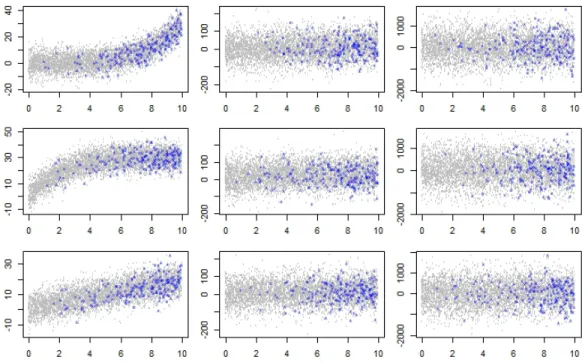
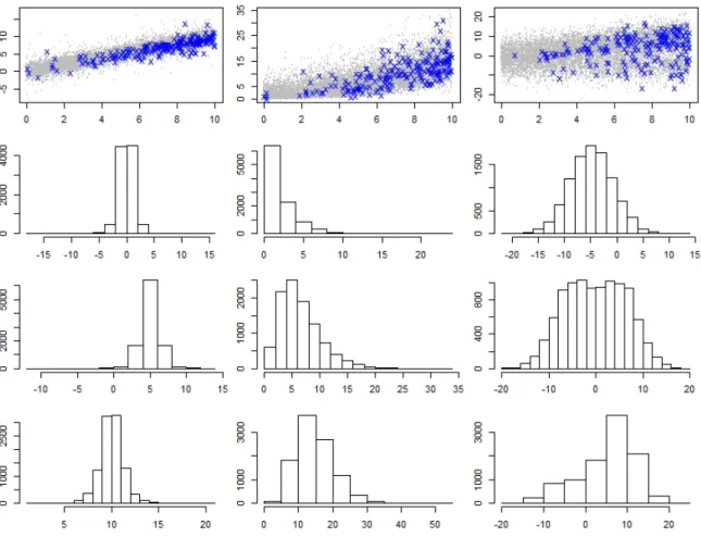
4.1 Scatter plot of generated population vs covariate. Population are marked grey in background and sample in blue cross. From left to right, σ2 = 101.5,103.5,105.5; from top to bottom, setting βa,βb,βc. . 72 4.2 Plot of quantile regression simulation settings. Population as grey in

background and sample in blue cross. From left to right: t distribu-tion, exponential distribution and bimodal distribution; From top to bottom: Scatter plot, Histogram of Y at X=0, 5, and 10. . . 77 4.3 Figure of biases of estimated population slope for median from all

three methods. Biasness of point estimates from each simulation are plotted sequentially. Blue circles mark the unweighted quantile regression, black crosses mark the fully weighted quantile regression, and red circles mark WDPM estimates. . . 82 4.4 Quantile regression of log TCDD on age. Sample presented as

back-ground dots, color represents weighting in log form, and lines from top to bottom are linear slope for first quartile, median and third quartile, black for WDPM, blue for fully-weighted . . . 87

(7)

LIST OF TABLES

Table

2.1 Bias, RMSE, and coverage of nominal 95% confidence/credible in-terval for linear slope when true model is linear and probability of selection is associated with slope: unweighted, fully weighted, stan-dard weight pooling estimator (without and with fractional Bayes Factor priors), linear spline weight pooling estimator (without and with fractional Bayes Factor priors), and generalized design-based estimator. . . 21 2.2 Bias, RMSE, and coverage of nominal 95% confidence/credible

in-terval for linear slope when true model is convex and probability of selection is associated with slope: unweighted, fully weighted, stan-dard weight pooling estimator (without and with fractional Bayes Factor priors), linear spline weight pooling estimator (without and with fractional Bayes Factor priors), and generalized design-based estimator. . . 22 2.3 Bias, RMSE, and coverage of nominal 95% confidence/credible

in-terval for linear slope when true model is concave and probability of selection is associated with slope: unweighted, fully weighted, stan-dard weight pooling estimator (without and with fractional Bayes Factor priors), linear spline weight pooling estimator (without and with fractional Bayes Factor priors), and generalized design-based estimator. . . 24 2.4 Bias, RMSE, and coverage of nominal 95% confidence/credible

in-terval for linear slope when true model is convex and probability of selection is not associated with slope: unweighted, fully weighted, standard weight pooling estimator (without and with fractional Bayes Factor priors), linear spline weight pooling estimator (without and with fractional Bayes Factor priors), and generalized design-based estimator. . . 25

(8)

2.5 Bias, RMSE, and coverage of nominal 95% confidence/credible in-terval for linear slope when true model is concave and probability of selection is not associated with slope: unweighted, fully weighted, standard weight pooling estimator (without and with fractional Bayes Factor priors), linear spline weight pooling estimator (without and with fractional Bayes Factor priors), and generalized design-based estimator. . . 26 2.6 Bias and RMSE for linear slope estimated for age: unweighted, fully

weighted, standard weight pooling estimator, and linear spline weight pooling estimator (without and with fractional Bayes Factor pri-ors).Units present in parenthesis. . . 28 2.7 Bias and RMSE for linear slope estimated for gender: unweighted,

fully weighted, standard weight pooling estimator, and linear spline weight pooling estimator (without and with fractional Bayes Factor priors).Units present in parenthesis. . . 28 2.8 Bias and RMSE for linear slope estimated for age and gender:

un-weighted, fully un-weighted, standard weight pooling estimator, and linear spline weight pooling estimator (without and with fractional Bayes Factor priors).Units present in parenthesis. . . 29 2.9 Bias and RMSE for linear slope estimated for age, gender and

interac-tion: unweighted, fully weighted, standard weight pooling estimator, and linear spline weight pooling estimator (without and with frac-tional Bayes Factor priors).Units present in parenthesis. . . 30 3.1 Comparison of various estimators of slope B1 under βa linear spline

setting. Bias and RMSE under populations with residual variance 101.5, 103.5and 105.5from following model: unweighted, fully weighted, hierarchical weight smoothing, exchangeable random effect and weight prediction by y, degree 5 polynomial of y, linear combination of x and y, and degree 5 polynomial of x,y. . . 48 3.2 Comparison of various estimators of slope B1 under βb linear spline

setting. Bias and RMSE under populations with residual variance 101.5_{, 10}3.5_{and 10}5.5_{from following model: unweighted, fully weighted,} hierarchical weight smoothing, exchangeable random effect and weight prediction by y, degree 5 polynomial of y, linear combination of x and y, and degree 5 polynomial of x,y. . . 48

(9)

3.3 Comparison of various estimators of slope B1 under βc linear spline setting. Bias and RMSE under populations with residual variance 101.5, 103.5and 105.5from following model: unweighted, fully weighted, hierarchical weight smoothing, exchangeable random effect and weight prediction by y, degree 5 polynomial of y, linear combination of x and y, and degree 5 polynomial of x,y. . . 49 3.4 Comparison under model misspecification. Bias and RMSE under

populations with underlying model quadratic coefficient 0, .45 and

.80 from following model: unweighted, fully weighted, hierarchical weight smoothing, exchangeable random effect and weight prediction by y, degree 5 polynomial of y, linear combination of x and y, and degree 5 polynomial of x,y. . . 52 3.5 Comparison under informative sampling. Bias and RMSE under

pop-ulations with correlation between Z and Y equal to .05, .50 and .95 from following model: unweighted, fully weighted, hierarchical weight smoothing, exchangeable random effect and weight prediction by y, degree 5 polynomial of y, linear combination of x and y, and degree 5 polynomial of x,y. . . 53 3.6 Regression of log TCDD on Age. Bias and RMSE for linear slope

estimated for age: unweighted, fully weighted and hierarchical weight smoothing. . . 55 3.7 Regression of log TCDD on Gender. Bias and RMSE for linear slope

estimated for gender: unweighted, fully weighted and hierarchical weight smoothing. . . 55 3.8 Regression of log TCDD on age and gender. Bias and RMSE for linear

slope estimated for age and gender: unweighted, fully weighted and hierarchical weight smoothing. . . 55 3.9 Regression of log TCDD on age and gender, and interaction between

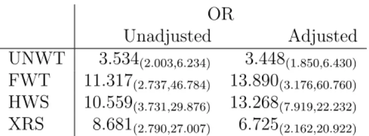
age and gender. Bias and RMSE for linear slope estimated for age, gender and interaction: unweighted, fully weighted and hierarchical weight smoothing. . . 56 3.10 Odds ratio and relevant 95% confidence interval for estimated effect

on injury from compacted extended cab pickups: unweighted, fully weighted, hierarchical weight smoothing and exchangeable random effect. . . 58

(10)

4.1 Comparison of various estimators of slope B1 under βa linear spline setting. Bias and relative RMSE under populations with residual variance 101.5, 103.5 and 105.5 from following model: Unweighted, Fully Weighted, Weight Trimming and weighted Dirichlet Process Mixture Model. . . 74 4.2 Comparison of various estimators of slope B1 under βb linear spline

setting. Bias and relative RMSE under populations with residual variance 101.5, 103.5 and 105.5 from following model: Unweighted, Fully Weighted, Weight Trimming and weighted Dirichlet Process Mixture Model. . . 74 4.3 Comparison of various estimators of slope B1 under βc linear spline

setting. Bias and relative RMSE under populations with residual variance 101.5, 103.5 and 105.5 from following model: Unweighted, Fully Weighted, Weight Trimming and weighted Dirichlet Process Mixture Model. . . 74 4.4 Comparison across various estimators of slope B1 under non central

T distribution. Bias and relative RMSE of estimates for 1st quartile, median and 3rd quartile of the outcome from following model: Un-weighted, Fully Weighted, Weight Trimming and weighted Dirichlet Process Mixture Model. . . 78 4.5 Comparison across various estimators of slopeB1 under Gamma

dis-tribution. Bias and relative RMSE of estimates for 1st quartile, me-dian and 3rd quartile of the outcome from following model: Un-weighted, Fully Weighted, Weight Trimming and weighted Dirichlet Process Mixture Model. . . 78 4.6 Comparison across various estimators of slopeB1 under Bimodal

dis-tribution. Bias and relative RMSE of estimates for 1st quartile, me-dian and 3rd quartile of the outcome from following model: Un-weighted, Fully Weighted, Weight Trimming and weighted Dirichlet Process Mixture Model. . . 79 4.7 Comparison across various estimators of slopeB1 under Bimodal

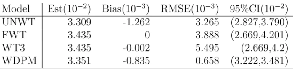
dis-tribution with Binary covariates. Bias and RMSE of estimates for 1st quartile, median and 3rd quartile of the outcome from following model: Unweighted, Fully Weighted, Weight trimming by 3 SD and weighted Dirichlet Process Mixture Model. . . 81 4.8 Regression of log TCDD on Age. Bias, RMSE and 95% CI for linear

slope estimated for age in unweighted, fully weighted, weight trim-ming by 3 SD and weighted Dirichlet Process Mixture models. . . . 84

(11)

4.9 Regression of log TCDD on Gender. Bias, RMSE and 95% CI for lin-ear slope estimated for gender in unweighted, fully weighted, weight trimming by 3 SD and weighted Dirichlet Process Mixture models. . 84 4.10 Regression of log TCDD on Age and Gender. Bias, RMSE and 95%

CI for linear slope estimated for age and gender in unweighted, fully weighted, weight trimming by 3 SD and weighted Dirichlet Process Mixture models. . . 85 4.11 Regression of log TCDD on Age, Gender and Interaction. Bias,

RMSE and 95% CI for linear slope estimated for age, gender and interaction in unweighted, fully weighted, weight trimming by 3 SD and weighted Dirichlet Process Mixture models. . . 85 4.12 Quantile regression of log TCDD on age. Bias, RMSE and 95%CI for

linear slope estimated for age in unweighted, fully weighted, weight trimming by 3 SD and weighted Dirichlet Process Mixture models. . 87 4.13 Quantile regression of log TCDD on gender. Bias, RMSE and 95% CI

for linear slope estimated for gender in: unweighted, fully weighted, weight trimming by 3 SD and weighted Dirichlet Process Mixture model. . . 88 4.14 Quantile regression of log TCDD on age and gender. Bias, RMSE and

95% CI for linear slope estimated for age and gender in unweighted, fully weighted, weight trimming by 3 SD and weighted Dirichlet Pro-cess Mixture models. . . 89 4.15 Quantile regression of log TCDD on age, gender and interaction.

Bias, RMSE and 95% CI for linear slope estimated for age, gender and interaction in unweighted, fully weighted, weight trimming by 3 SD and weighted Dirichlet Process Mixture model. . . 91

(12)

LIST OF APPENDICES

Appendix

A. Metropolis Algorithm For Advanced Weight Pooling Method . . . 98 B. Gibbs Sampler For Weight Smoothing Model . . . 101 C. Gibbs Sampler for Weighted Dirichlet Process Mixture Model with

(13)

ABSTRACT

Robust and Efficient Methods for Bayesian Finite Population Inference by

Xi Xia

Chair: Professor Michael R. Elliott

Bayesian model-based approaches provide data-driven estimates of population quan-tity of interest from complex survey data to achieve balance between bias correction and efficiency. We focus on the issue of accommodating sample weights equal to the inverse of the probabilities of inclusion. In settings with highly variable weights, weight “trimming” is often employed in an ad-hoc manner to decrease variance, while possibly increasing bias. We consider three model-based methods to provide princi-pled bias-variance tradeoffs.

Weighted estimators can be developed in a model-based framework by including interactions between the quantity of interest (e.g., mean, regression parameters) and the weights; weight pooling builds a variable selection model where these interactions are dropped for differing values of the weights; and estimation proceeds using the posterior distribution of model averages. The extension considers a weight pooling linear spline model that uses a linear spline to capture regression coefficient patterns for all strata, and collapses together the strata with minor differences. Our model achieves robustness when weights are needed to guard against model misspecification, and efficiency when weight-coefficient interactions could be ignored. We also model

(14)

the interactions between the weights and the estimators of interest as random effects, reducing the overall RMSE by shrinking interactions toward zero when such shrinkage is supported by data (Elliott and Little 2000, Elliott 2007). We adapt a flexible Laplace prior distribution to gain robustness against model misspecification. We find that weight smoothing models with Laplace priors approximate unweighted estimates when weighting is not necessary, and could greatly reduce the RMSE if strong pattern exists in data in linear model setting. Under logistic regression with same sample size, the estimates are still robust, but with less gain in efficiency. Finally, we adapt a Dirichlet process mixture (DPM) model that is capable of approximating highly-skewed and multimodal distributions, often with small number of components. The extended weighted DPM version allows the DP prior to be a mixture of DP random basis measures that is a function of covariates, extends applications to regression, and creates a natural link to survey weights. We also investigate its application to inference for quantile regression, providing a new approach for quantile regression incorporating complex survey design. Simulation results suggest great reduction in RMSE from weighted DPM method under most of the scenarios.

(15)

CHAPTER I

Introduction

When analyzing data with complex survey design, biasness in estimating the quantity of interest (population mean, slope, etc.) is often introduced by unequal probabilities of inclusion, and fully-weighted estimators with weights equal to the inverse of probabilities of inclusion are the common countermeasure to correct bias-ness. Obtained by applying weights in score equations and forming pseudo-maximum likelihood estimators (PMLEs), the fully-weighted estimator is design consistent for MLEs, either as defined in Cochran (1977) – the estimator equals the population quantity being estimated when the sample consists of the whole population – or as defined in Sarndal (1980) – the estimator converges to the target quantity where samples of increasing size are selected in an identical fashion from infinite replicates of the population. However, this welcome property can come at the cost of increase in the variance of estimator. When quantity of interest is not related to weights, or extreme values of weight exist, the gain in bias-reduction may not compensate the loss due to increasing variance, leading to an overall larger mean square error (MSE). To reduce the inflated variance in that situation, various methods have been pro-posed. One general approach, weight trimming, or winsorization, limits the influence from extreme weights by capping the weights at some cut point w0, and redistribut-ing the trimmed values equally among the rest (Alexander et al., 1997; Kish, 1992;

(16)

Potter, 1990). This leads to various extensions in deciding the cut pointw0. Some ex-amples include the NAEP method by Potter (1988), which set the cutoff point equal

p cP

i∈sw 2

i/n, where c is chosen in an ad-hoc manner; the empirical MSE method byCox and McGrath (1981) which estimates the cutoff point value by optimizing the empirical MSE estimated fromM SEˆ ( ˆθt) = ( ˆθt−θˆw)2−V arˆ ( ˆθt)+2

q

ˆ

V ar( ˆθt) ˆV ar( ˆθw), where ˆθw is the fully weighted estimator, and ˆθt, t= 1, ..., T, is the weight trimmed estimator, witht denoting various trimming levels, from 1 as the unweighted estima-tor toT as the fully-weighted estimator; and the skewed CDF method by Chowdhury et al. (2007), which assumes a skewed cumulative distribution (e.g., an exponential distribution) on the weights, and uses the upper 1% of the fitted distribution as a cut point for weight trimming. Details of these approaches are summarized in Henry and Valliant (2012) review.

An Alternative approach we focus on here is the Bayesian model-based approach, in particular finite population Bayesian inference that provides data-driven estimates that balance bias and efficiency. The Bayesian approach posits a model, parametric or nonparametric, as a prior distribution for the fixed and unknown finite population that depends on unknown parameters. Inference about the quantity of interest as a function of the population is made by summarizing the posterior predictive distribu-tion of unobserved observadistribu-tions in the populadistribu-tion. It is an attractive feature which Bayesian model-based approach does not rely on asymptotic arguments.

To account for survey designs with disproportional selection probabilities under a Bayesian framework, one can create dummy indicators that stratify samples by equal or approximately equal probabilities of selection. And a fully-weighted data analysis is equivalent to estimating a model with interactions between stratum indicators and target model parameters of interest. However, as number of strata increases, the numbers of interaction terms increase accordingly, reduce efficiency of the interaction model, or even make it impossible to estimate all parameters under extreme

(17)

circum-stances. Thus, varies models are proposed that are simpler than the full interaction model, but still maintain enough flexibility to accommodate different population pat-terns precisely and yield better inferences. In the following chapters, we study these models and expand their applications.

In chapter II, we extend the “weight pooling” models ofElliott and Little (2000);

Elliott (2007, 2008) that provides analog of the standard weight trimming method, adapted to a more principled Bayesian model framework. Note that a fully-weighted data analysis can be viewed as inference from the posterior predictive distribution of a population quantity under a model in which interaction terms are presented be-tween the weight stratum indicators and the underlying model parameters of interest. Weight pooling drops unnecessary interactions based on different values of weights in a data-driven manner. Inference is based on averaging all possible weight pooling models based on their posterior probabilities of being “correct”. The early version in Elliott and Little(2000) merged together only strata with largest weights, assuming the underlying data in these combined strata are exchangeable. Later, by consid-ering the possibility of pooling all contiguous strata, Elliott (2008, 2009) introduced higher degree of robustness into the model, and protected against ”over-pooling” that occurred in the earlier version.

To further extend the model’s capability in handling complex association between strata and quantity of interest, we construct a linear spline model with potential knots to capture regression coefficient patterns for all strata, and collapse together strata with minor differences. Also, with large number of knots considered, we apply a Metropolis step to move around the potential model space, in contrast to previ-ous approaches that required computing posterior probabilities of all possible pooling models, and greatly reduce the burden in computing. Furthermore, we apply a Frac-tional Bayes Factor prior (O’Hagan, 1995) to boost the model’s performance. We assess our new method in a simulation study that aims at estimating population slope

(18)

under various data patterns, competing against unweighted estimate, fully weighted estimate and different weight trimming methods. Bias, RMSE and coverage rate are recorded, and the results suggest that our method maintains consistent better performance regarding RMSE.

In chapter III, we study the “weight smoothing” approach that estimates popula-tion quantity of interest through mixed models that consider interacpopula-tions between the weights and the quantities of interest as random effects, shrinking them towards zero when data provide little evidence of interactions, but keeping strata separated when data suggest interacting (Elliott, 2007; Elliott and Little, 2000; Ghosh and Meeden, 1986;Lazzeroni and Little, 1998;Little, 1991, 1993;Rizzo, 1992). Elliott (2008, 2009) extended the application to linear and generalized linear models, and discussed four different settings for the random effect priors, namely exchangeable, autoregressive, linear and nonparametric random slopes, and evaluated their performances.

We adapt a more flexible Laplace prior distribution instead of multivariate nor-mal distribution for the hierarchical Bayesian model in order to achieve more robust-ness against “oversmoothing” in settings where weights are required to accommodate model misspecification or non-ignorable sampling. Given the prevailing performance of Laplace prior in sparse model selection, we expect the hierarchical model to main-tain high performance, even under simplistic mean and covariance matrix settings such as exchangeable random priors, therefore reduce the overall complexity of the model. Again, we test the performance of our proposed model in simulation stud-ies, under both model misspecification and informative sampling settings, for both numerical and dichotomous outcomes, and compare it with competing methods. De-spite some minor decrease in coverage rates, our method performs consistently better than the competing methods, reducing RMSE by up to 50% in certain settings.

In Chapter IV, we introduce the Dirichlet Process Mixture model (Dunson et al., 2007) in complex survey data analysis. Depicting interactions between regression

(19)

pa-rameters and probabilities of inclusion by a combination of fixed number of component distributions, the Gaussian mixture model is known for approximating highly-skewed and multimodal distributions, often with fairly small number of components. DPM model relaxes the assumption of pre-determined number of mixture components. The extended Weighted Dirichlet Process Mixture Model (WDPM meodel) further allows the DP prior to be a mixture of DP random basis measures that is a function of covari-ates, granting more flexibility to extend applications to mean of quantile regression models.

In this manuscript, we investigate the application of the WDPM model in an-alyzing complex survey design data with small sample sizes, targeting data-driven inference that captures a wide variety of normal and non-normal distributions, in a fashion that is sensitive to unequal probability of selection aspects of the sample design, but also offers increased efficiency when data permit. In additional to the linear regression setting, we also consider applications to quantile regression. Due to the fact that the WDPM models are highly flexible and can generate predictive distributions that are accurate in tails of the distribution, they are a natural choice to consider for model-based methods to obtain population quantile regression estimates. To evaluate the performance of the WDPM models, we run a series of simulations across various mis-specified models and non-normal distributions, under both linear model and quantile regression settings. The results show considerable improvement compared to fully weighted methods across all settings tested.

Besides simulations, we also test all three models’ performances with Dioxin Dataset from NHANES study, focusing on identifying the relationship between log transformed 2,3,7,8 tetracholorodibenzo-p-dixoin (TCDD), a toxic substance that ac-cumulates in blood, and demographic factors like gender and age. The fully-weighted estimates are assumed to be the true values, and bias, RMSE are calculated ac-cordingly. To evaluate the extended application in generalized linear regression from

(20)

chapter III, we apply the method on Partner of Child Passenger Safety Dataset from State farm Insurance database, featuring the status of cars involved in accident, and the injury status of their children passengers. The outcome variable is a binary in-jury index, and predictors are various car status. We still observe some improvement from our proposed methods, but less clearly compared to well-controlled simulation studies.

(21)

CHAPTER II

Advancements in “Weight Pooling” Approaches to

Reduce Mean Square Error in Weighted

Estimators

2.1

Introduction

When analyzing data for sample designs with unequal probabilities of inclusion, standard design-based approaches typically use “fully-weighted” estimates of popula-tion means, totals, regression slopes, etc., where the weights are equal to the inverse of the probabilities of inclusion (Horvitz and Thompson, 1952). The fully-weighted estimators of model parameters obtained by using sampling weights in score equations are sometimes termed “pseudo-maximum likelihood” estimators (PMLEs) (Binder, 1983; Pfeffermann, 1993) because they are design consistent for MLEs that would solve the score equations under the data modelf(Y |θ) if we had observed data for the entire population. While design consistency, either in the sense of Cochran (1977) – the estimator equals the population quantity being estimated when the sample con-sists of the whole population – or in the asymptotic sense of Sarndal (1980), where asymptotics are formed from samples selected in an identical fashion from t → ∞ replicates of the population, is an attractive property, bias reduction typically comes at the cost of increased variance. This increase can overwhelm the reduction in bias,

(22)

so that the mean square error (MSE) actually increases under weighted analysis. An alternative to standard design-based procedures is to use model-based proce-dures, in particular finite population Bayesian inference. Design-based inference in survey data analysis treats the survey outcome variables Y = {Y1, Y2, . . . , YN} for

N subjects in the population as fixed unknown constants; the random process is the sample design which identifies thensample subjects in the population. An estimate of the population quantity Q=Q(Y) is constructed based on the sample q =q(Yobs), a function of the sample Yobs ={y1, y2, . . . , yn}. In contrast, Bayesian approaches posit a model for the population data Y as a function of parameters θ: Y ∼ f(Y | θ, Z), where Z designates the design variables. This is treated as prior distribution for the fixed and unknown finite population Y depending on some unknown parameter θ. This prior distribution can be parametric or nonparametric. Inference aboutQ(Y) is made on the posterior predictive distribution ofp(Ynob |Yobs, I, Z), whereYnobconsists of the N −n unobserved quantities in the population Y:

p(Ynob |Yobs, I, Z) =

R R

p(Ynob |Yobs, Z, θ, φ)p(I |Y, Z, θ, φ)p(Yobs |Z, θ)p(θ, φ)dθdφ

R R R

p(Ynob |Yobs, Z, θ, φ)p(I |Y, Z, θ, φ)p(Yobs |Z, θ)p(θ, φ)dθdφYnob

(2.1) where φ models the inclusion indicator I. If we assume that φ and θ are priori independent and if the distribution of I is independent of Y|Z, the sampling design is said to be “unconfounded” or “noninformative”; if the distribution of I depends only on Yobs|Z, and p(θ, φ) = p(θ)p(φ), then the sampling mechanism is said to be “ignorable” (Rubin, 1987). Under ignorable sampling designs, p(I |Y, Z, θ, φ) =p(I |

Yobs, Z, φ), and thus (2.1) reduces to

R

p(Ynob |Yobs, Z, θ)p(Yobs |Z, θ)p(θ)dθ

R R

p(Ynob |Yobs, Z, θ)p(Yobs |Z, θ)p(θ)dθdYnob

=p(Ynob |Yobs, Z),

(23)

inclusion parameterI (Ericson, 1969;Holt and Smith, 1979;Little, 1993;Rubin, 1987;

Skinner et al., 1989). Under the Bayesian approach, the posterior distribution – the conditional distribution of parameters of interest given data – is used for all purposes. This is an attractive feature of a Bayesian method in that it offers conditional inference given data and does not rely on asymptotic arguments.

To accommodate disproportional probability-of-selection designs in a Bayesian framework, case weights can be transformed into dummy variables that stratify by equal or approximately equal probabilities of inclusion, ordered by the inverse of the probability of inclusion (Holt and Smith, 1979). Then, a fully-weighted data analysis estimates the posterior predictive distribution of a population quantity under a model in which interaction terms are present between weight stratum indicators and under-lying model parameters of interest. Elliott and Little (2000) and Elliott (2007, 2008, 2009) developed model-based estimators for weight trimming using two broad ap-proaches: Bayesian hierarchical modeling, or “weight smoothing,” and Bayesian vari-able selection modeling, or “weight pooling.” “Weight smoothing” models treat the underlying weight strata as random effects, and induce weight trimming by smooth-ing strata for which the data provide little evidence of difference, and separatsmooth-ing strata that the data suggest should be separated (Elliott, 2007; Elliott and Little, 2000; Ghosh and Meeden, 1986; Lazzeroni and Little, 1998; Little, 1991, 1993; Rizzo, 1992). “Weight pooling” models collapse together inclusion strata. Collapsing only the largest valued strata mimics weight trimming by assuming the underlying data from these combined strata are exchangeable. By averaging over all possible of these “weight pooling” models, we can compute an estimator of the population parameter of interest whose bias-variance tradeoff is data-driven. By allowing for all contigu-ous inclusion strata to be considered for pooling, Elliott (2008, 2009) induced a high degree of robustness into this model, protecting against ”over-pooling” that simpler models suffered from Elliott and Little (2000).

(24)

Here we extend the weight-pooling method from Elliott (2008, 2009) in two ways. First, we borrow from the weight-smoothing approach, constructing a linear spline model with many potential knots to grant more flexibility to handle non-linear associ-ations. Second, in contrast to previous approaches that require computing directly the posterior probabilities of all possible models, we use a Metropolis step to move around the potential model space, allowing a much larger number of weight strata combina-tions to be considered. We test the properties of our proposed approach through simulation, comparing it with competing methods recently proposed for data-driven weight trimming. We also apply the method to determine the relationship between dixon blood level and age and gender using data from the 2003-2004 National Health and Nutrition Examination Survey (NHANES).

This Chapter is organized as follows. In Section 2 we review traditional weight trimming methods as well as recently proposed model-assisted and model-based meth-ods, and develop our proposed linear spline model. Section 3 presents the results of the simulation studies, comparing bias, coverage, and MSE of the proposed method and the competing methods. In Section 4 we evaluate the method through applica-tion to the NHANES survey. In secapplica-tion 5 we discuss possible direcapplica-tions for further study.

2.2

Weight Pooling Method

2.2.1 Weight Trimming

When weights are overly variable, they are commonly trimmed or “winsorized” so that weights larger than some value w0 are fixed as w0, with the values above w0 distributed among the rest (Alexander et al., 1997; Kish, 1992; Potter, 1990). Some approaches have been developed that focus on determining the cap valuew0 based on

(25)

data. These include the NAEP method by Potter (1988), which determines the cutoff point aspcP

i∈sw 2

i/n, wherecis empirically chosen according tonw2i/

P

i∈sw 2 i. Cox and McGrath (1981) proposed an empirical MSE approach that relies on optimizing the empirical MSE ofM SEˆ (¯yt) = (¯yt−y¯w)2+ ˆV ar(¯yt)+2

q

ˆ

V ar(¯yt) ˆV ar(¯yw), t= 1...T, where t denotes various trimming level, from 1 as unweighted estimator to T as fully-weighted estimator. Chowdbury et al. (2007) approached the problem by assuming the weights follow a skewed cumulative distribution, such as exponential distribution, and determining the cut point by the upper 1% of the fitted distribution. For more details of these approaches, see review of design-based weight trimming methods in Henry (2012).

2.2.2 Weight Prediction

Beaumont (2008) proposed a design-based, model-assisted method, considering a prediction model of weights using a polynomial form of a response variable and design variables. Assuming a prediction model for weights, and allowing response variable and design variables in the model, the predicted weights from the fitted model tamp down extreme values. To be more specific, denote I = (I1, ...IN)T as the vector of sample inclusion indicators, i.e. Ii = 1 as ith unit sampled and

Ii = 0 otherwise, Y = (Y1, ...YN)T the vector of survey response variable, and

Z = (Z1, ...ZN)T the vector of design variables. Also it is assumed that the prob-ability of sampling is noninformative, thus P(I|Z, Y) = P(I|Z). The smoothed weights are obtained from ˜wi = EM(wi|Ii, zi, yi), where EM(·) denotes expectation taken with respect to the model for the weight. Beaumont also suggested dropping dependence on design variables, so that ˜wi = EM(wi|Ii, yi). Two estimators are proposed: a linear model, EM(wi|I, Y) = HiTβ +v

1/2

i i, and an exponential model,

EM(wi|I, Y) = 1 +exp(HiTβ+v 1/2

i i), whereHi and vi >0 are known functions ofyi. The latter model prevents the predicted weights from being negative. Two examples

(26)

of H functions are given as well, respectively linear combination of yi and a degree five polynomial of yi. Once the predicted weights are obtained by fitting the model to the sampled data, the re-weighted estimator of interest is created.

By including the design variables in the model, Beaumont’s suggested method incorporates more information and yields improved prediction of weights for the weighted mean and population estimators. Yet the method does not actually fo-cus on assessing the degree of uncertainty associated with the relationship between the probability of selection and the sample statistic of interest. Large degrees of uncertainty suggest that maintaining such relationships, at least in an unattenuated form, may add variance in excess of any bias correction. Hence a stronger link be-tween weights and the covariate effects could be considered, and a more efficient form of prediction model obtained, which is the approach we pursue in this manuscript.

2.2.3 Weight Pooling

The traditional weight trimming method effectively reduces variance by constrain-ing weights to certain capped value w0 (often chosen to be 3 or 6 times than mean weight ¯w = n−1P

iwi), and redistributing the extra weights among uncapped ones by multiplying them by a normalizing constant γ = (N+−

P

κiwo)/

P

(1−κi)wi, where κi is an indicator variable for whether or not wi ≥ w0. To put this in a modeling context, consider a disproportionally stratified design, and focus on the population mean as the value of interest. The weighted estimator is then defined as ¯ yw = P hwhPnhi yhi P hnhwh = P

h(Nh/N) ¯yh, wherewh =Nh/nh is the inverse of the probabil-ity of selection in stratumh, andnh and Nh correspond to the sample and population size in stratum h respectively. It is straighforward to show that ¯yw is the posterior mean of Gaussian model that assumes different means for each stratum and a constant

(27)

variance, with non-informative priors (Elliott and Little 2000):

Yhi|µh ∼N(µh, σ2)

µh, µl,logσ ∝const.

The trimmed weight mean estimator is given by

y_wt = l−1 X h=1 γNh N+ y_h+ H X h=l w0nh N+ y_h = γ l−1 X h=1 Nh N+ y_h+w0 PH h=lnh N+ y(l) where γ = N+−w0PHh=lnh Pl−1 h=1Nh and y(l) = (1/PH h=lnh) PH h=lnhyh. Choosing w0 = PH h=lNh PH h=lnh yieldsγ = 1 andy_wt=Pl−1 h=1 Nh N+yh+ (PHh=lNh) N+ y

(l)_{; the resulting trimmed weight mean} corresponds to the estimate for a model that assumes distinct stratum means for the smaller weight strata and a common mean for the larger weight strata above a cut point l (Elliott and Little 2000):

Yhi|µh ∼N(µh, σ2)h < l

Yhi|µl∼N(µl, σ2)h ≥l

µh, µl,logσ∝const

Elliott and Little (2000) proposed a model-based approach, where the cut pointl was no longer a known constant, but a data-driven parameter. The hierarchical model is

(28)

written as following: Yhi|µh ∼N(µh, σ2)h < l Yhi|µl∼N(µl, σ2)h ≥l P(L=l) = 1/H P(σ2|L=l) =σ−(l+1/2) P(β|σ2, L=l) = 2π−l

where µ1 = β0, µl = β0 + βl−1, and L indicates the selected pooling model. Via

Bayesian model averaging, a posterior distribution of L is determined, and the esti-mated mean is obtained by summarizing estimations from all models. By averaging based on the probability of certain potential pooling model been the true model, the method avoids the possibility of relying on one single misspecified model, and gains robustness.

Elliott (2008, 2009) extended the method to a linear and generalized model re-gression setting ofYi on fixed covariatesXi. By allowing interactions between weights and the population slope, the model could mimic either a fully-weighted estimator or an unweighted estimator, depend on whether the full interaction model or minimal model (all strata share the same slope) been selected. Any model between the two represents a degree of trimming determined by data. And by allowing any adjacent strata, rather than strata on the high end only, to collapse, it introduces more flex-ibility in modeling, thus potentially increasing the robustness. The model is given

(29)

by:

Yhi|xhi, βl, σ2, L=l∼N(Zliβl, σ2)

βl|σ2, L=l∼N(β0, σ2Σ0)

σ2|L=l ∼Inv−χ2(a, s2)

P(L=l) = 2−(H−1)

whereZli =Dhl⊗xhiandDhlis a vector of dummy variables indicates thelth pooling pattern.

2.2.3.1 Weight Pooling Linear Spline Model

The weight pooling method in Elliott (2008) identifies data patterns by either estimating separately the population statistic of interest in each weight stratum, or pooling together the strata to estimate the population statistic. Yet if the statistic follows an approximate linear pattern across these strata, the model may either fail to identify the pattern, or spend unnecessary degrees of freedom estimating it. To obtain further flexibility to balance between simple and complex underlying data structures, we propose a linear spline version of weight pooling, assuming the regression param-eters themselves follows a linear spline trajectory. This proposed method replaces the changepoint model above, which treats all regression parameters as being equal within pooled strata, with a linear spline model that assumes that the regression pa-rameters themselves follow a linear spline trajectory, with knots {τk} under the lth knot pattern (Zheng and Little, 2003, 2004, 2005):

E(yi |xi,βl, L=l) = p X j=0 " β_j0l + H∗ X k=1 β_jkl (h−τk)+ # xji (2.2)

where x0i ≡ 1 for all i (intercept term), (x)+ = x if x > 0, 0 otherwise, and H∗ is the number of knots in thelth knot pattern. A generalized linear model (GLM) can

(30)

be obtained by replacing with g(E(yi | xi,βl, L = l)), where g(·) is the GLM link function. Thus the unweighted analysis is obtained ifL= 1 so that τ1 =H:

β_j0l + H∗ X

k=1

β_jkl (h−τk)+ =β_j01 +β_j11 (h−H)+ =β_j01 , i∈h= 1, . . . , H

Conversely, the fully weighted analysis is obtained when L = 2H−1 so that τ1 = 1, ..., τH−1 =H−1 and H∗ =H−1: β_j0l + H−1 X k=1 β_jkl (h−τk)+ =                  β_j02H−1, i∈h = 1 β_j02H−1 +β_j12H−1, i∈h= 2 .. . β2H−1 j0 + (H−1)β2 H−1 j1 +· · ·+β2 H−1 j,H−1, i∈h=H as all interactions between the regression parameters and the weight strata are in-cluded. Intermediate pooling models provide mean structure under a flexible linear model, so that, ifL=l1(H−2) +l2 (changepoints atl1, l2,l1 < l2), thenH∗ = 2 and:

β_j0l + 2 X k=1 β_jkl (h−τk)+ =                        β_j0l∗, i∈h= 1, ..., l1−1 βl∗ j0+βl ∗ j1(h−l1) = (βl∗ j0−βl ∗ j1l1) +βl ∗ j1h, i∈h=l1, ..., l2−1 βl∗ j0+βl ∗ j1(h−l1) +βl ∗ j2(h−l2) = (βl∗ j0−βl ∗ j1l1−βl ∗ j2l2) + (βl ∗ j1+βl ∗ j2)h, i∈h =l2, ..., H for l∗ =l1(H−2) +l2.

We anticipate that this model should reduce the number of changepoints needed to pick up local non-linearities in the interactions between regression slopes and weights, while providing a more rapid tradeoff toward variance reduction when bias correction is unimportant but still retaining robustness. Note that the set of knots {τ1, ..., τH∗}

maps 1-1 with the model index L=l, so the prior on the knots corresponds to p(L). Also note that, if we denote Zi =xi(1,(h−τ1)+, ...,(h−τH)+)0, and βl= (β0, ...βH), the expected transformed mean of Yhi|xhi, βl, σ2, L=l can be written as Ziβ, which

(31)

resembles the format in Elliott (2008, 2009) for computation.

Assuming a generalized linear model with link functiong(µi) and variance function

V(µi) for E(Yi) = µi, our population quantity of interest B = (B1, . . . , Bp)T is the slope that solves the population score equation:

UN(B) = N X i=1 (yi−g−1(µi(B)))xi V(µi(B))g0(µi(B)) .

The posterior predictive distribution of B is then given by

p(B|y) = X l

Z Z

p(B|y,β_l, φ, L=l)p(β_l, φ |y, L=l)P(L=l|y)dβ_ldφ

Simulations from p(B | y, X) can be obtained by drawing first from P(L = l | y), then fromp(β_l, φ|y, L=l), and solving

H X h=1 Wh nh X i=1 (ˆyhi−g−1(µi(B)))xhi V(µhi(B))g0₍_µ_hi(_B₎₎ = 0

where Wh = Nh/nh for the population size Nh, sample size nh in the hth inclusion stratum, andZli =Dhl⊗xhi whereDhl is a vector of dummy variables that pool the appropriate conterminous inclusion strata based on the lth pooling pattern. Since the computation of the kernel of P(L|y, X) is applicable under conjugate prior, if

H is of moderate size, the factor between kernel and actual distribution could be achieved by summing up all kernels, and a direct draw from posterior probability

P(L|y, X) is possible. Alternatively, the ratio ofP(L|y, X) from two pooling patterns is always accessible since their distributions share the same constant factor. This leads to a Metropolis step to approximate the marginal posterior distribution P(L=

l|y, X), and direct draws of other parameters accordingly. The latter approach is computationally plausible under large H. We provide details of the Markov Chain Monte Carlo algorithm for the Gaussian linear regression setting in Appendix A.

(32)

2.2.3.2 Fractional Bayes Factor

During the Metropolis step of drawing P(L|y, X), we must compute the Bayes Factors(BF), comparing weight pooling model l with model l0:

BF(y, X) = p(L=l|y, X) p(L=l0_|_{y, X}₎ = p(y|L=l, X)p(L=l) p(y|L=l0_{, X}₎_p₍_L₌_l0₎ = R f(y|θl)p(θl)dθlp(L=l) R f(y|θl0)p(θ_l0)dθ_l0p(L=l0) .

Under weakly informative priors, the BF is usually quite sensitive to the choice of

p(θl) (Kass and Raftery, 1995). To counter this, we use the fractional Bayes Factor approach developed by O’Hagan (1995). The approach sets aside a fractionb of data for a data-based prior forθl, and the relevant fractional Bayes Factor(FBF) is defined as BFb(y, X) = ql(f, y, X)P(L=l)/ql0(f, y, X)P(L=l0), where ql(f, y, X) = R p(θl)f(y|θl)dθl R p(θl)f(y|θl)b_dθ l .

O’Hagan suggested n−1_log_n _and _n−1/2 _{as increasingly “robust” choices of} _b_{. The} former one is smaller, which would make the model sensitive to data structure, while the latter with larger value leads to more robust model selection against possible outliers (data generated under a model not in the classes considered).

2.3

Simulation Study

We explore the linear spline weight pooling model in linear regression setting via a set of simulation studies. We consider two basic settings: one in which the probability of selection is associated with the linear approximation between the outcome Y and the predictor of interestX, and one in which the probability of selection is independent of this linear approximation.

(33)

2.3.1 Association between Probability of Selection and Regression Slope

Here we generate the population under a model similar to Elliott (2008), but extended to 20 strata: yi|xi, β, σ2 ∼N(β0 + 20 X h=1 βh(xi−h)+, σ2) xi ∼U N I(0,10), i= 1, ..., N, N = 20,000.

The sample design is a disproportionally stratified model, with 20 strata where the probability of selection within each stratum is given by:

P(Ii|Hi) = πi ∝(1 +Hi/15)Hi

Hi =d2Xie/2.

Note that the probability of selection is related to regression covariate.

The probabilities of inclusion are constructed that the ratio between the maximum and minimum of weights is around 35, and the sizes of potential strata are greater than 3 to be estimable. A total number of 1000 elements are sampled without replacement for each simulation. Our target estimator is the best linear approximation of the linear slope B2 relatingY toX, given by

   B1 B2   = N X i=1 XiXiT !−1 _N X i=1 Xiyi

where Xi = (1 xi), The number of possible weight pooling models is given by 219 = 524,288, far too many to be averaged over directly as in Elliott (2008).

(34)

For simulation settings we consider three β patterns:

1.βa = (0,2,0,0,0,0,0,0,0,0,0,0,0,0,0,0,0,0,0,0,0)0 2.βb = (0,0,0,0,0,0, .5, .5, .5, .5,1,1,1,1,2,2,2,2,4,4,4)0

3.βc = (0,22,−4,−4,−2,−2,−2,−2,−1,−1,−1,−1,−.5,−.5,−.5,−.5,0,0,0,0,0)0

which represent respectively a pure linear model, an increasing curve, and a flattening curve. Under βa where ordinary linear model is correctly specified, the weights are not needed for bias correction, so the unweighted estimator should be most efficient. Under βb, the unweighted estimator is biased, but the most non-linear part of the model space is the most heavily sampled, somewhat dampening the variance inflation for fully-weighted estimator. Under βc, correction of bias is also necessary, but the most non-linear part of the model space is the least sampled, inflating the variance of the fully-weighted estimator. Population varianceσ2 _{varied as 10}l_,_l_{= 1}_.₅_,₃_.₅_,₅_._5, emphasizing different degrees of bias-variance tradeoff. 200 simulations are generated under each β and σ2 combination.

We apply data-based priors for the regression parameters, centering them at the unweighted value with a very inflated variance: β0 = ˆβ = (XTX)−1XTy, Σ0 =

cnV ar( ˆβ) for V ar( ˆβ) = ˆτ2₍_XT_X₎−1_{, ˆ}_τ2 _{= (}_n ₋_p₎−1₍_y ₋_X_β_ˆ₎T₍_y ₋_X_β_ˆ_{), where}

c = 1000. For the the variance prior, we assume a = s = 10−8_{. We also consider} Fractional Bayes Factor priors with training fraction of logn/nand n−1/2_.

To evaluate the estimation of population slope, we consider a comparison among an unweighted model (UNWT), a fully weighted model (FWT), the Elliott (2008) weight pooling method (PWT) and the Fractional Bayesian Factor versions (PWTFBF1 and PWTFBF2 corresponding to b =n−1_log_n _and _b ₌_n−1/2 _{respectively), the} lin-ear spline version of weight pooling developed in this manuscript (PWTLS), and their respective Fractional Bayesian Factor versions. We also consider the

(35)

general-Bias RMSE relative to FWT 95% Coverage Modelσ2(log10) Modelσ2(log10) Modelσ2(log10)

Estimator 1.5 3.5 5.5 1.5 3.5 5.5 1.5 3.5 5.5 UNWT -0.027 0.081 -0.201 0.753 0.701 0.694 0.93 0.96 0.96 FWT -0.018 0.137 0.254 1 1 1 0.96 0.93 0.97 PWT -0.018 0.135 0.243 1.037 1.012 1.004 0.98 0.95 0.98 PWTFBF1 -0.015 0.129 -0.037 0.853 0.811 0.810 1 0.98 0.98 PWTFBF2 -0.015 0.128 0.035 0.946 0.912 0.911 0.99 1 0.99 PWTLS -0.013 0.163 0.031 0.914 0.942 0.917 0.99 0.98 0.98 PWTLSFBF1 -0.016 0.131 -0.372 0.815 0.770 0.793 1 1 1 PWTLSFBF2 -0.014 0.172 -0.165 0.815 0.817 0.849 1 1 1 WT1Y -0.011 0.131 -0.248 0.753 0.708 0.706 0.96 0.98 0.94 WT5Y 0.092 0.391 -0.256 1.374 0.833 0.707 0.71 0.89 0.94 WT5YX 0.071 0.165 -0.153 1.196 0.810 0.795 0.74 0.91 0.92 WT5Y5X -0.018 0.136 -0.241 0.935 0.911 0.928 0.96 0.96 0.98 Table 2.1: Bias, RMSE, and coverage of nominal 95% confidence/credible interval

for linear slope when true model is linear and probability of selection is associated with slope: unweighted, fully weighted, standard weight pooling estimator (without and with fractional Bayes Factor priors), linear spline weight pooling estimator (without and with fractional Bayes Factor priors), and generalized design-based estimator.

ized design-based estimator from Beaumont (2008) as a competing method, where the choice of functionH varies fromy(WT1Y), degree five polynomial of y(WT5Y), degree 5 polynomial of y plus x (WT5YX), to degree 5 polynomial of y and x sepa-rately (WT5Y5X). Under each setting, the estimators are compared with respect to bias, RMSE, and nominal 95% coverage rate, where RMSE is presented as relative to the fully weighted estimator. Results are provided in Tables 2.1, 2.2, and 2.3.

Under βa, the linear model is correctly specified, all estimators are unbiased, and as expected the unweighted estimator has the best performance, maintaining ap-proximately 70% RMSEs comparing to fully-weighted estimator at all values of σ2 considered, together with approximately correct coverage rates. The standard weight pooling estimator has results that closely parallel to the fully-weighted estimator; it is substantially improved by applying FBF, reducing RMSEs relative to the fully-weighted one by approximately 20% for FBF1 and 10% for FBF2 while maintaining

(36)

Bias RMSE relative to FWT 95% Coverage Model σ2(log10) Model σ2(log10) Model σ2(log10)

Estimator 1.5 3.5 5.5 1.5 3.5 5.5 1.5 3.5 5.5 UNWT 2.514 2.483 2.216 10.474 2.785 0.748 0 0 0.91 FWT -0.011 0.151 0.243 1 1 1 0.98 0.95 0.98 PWT -0.010 0.152 0.304 0.391 0.972 1.002 1 0.94 0.99 PWTFBF1 0.005 0.284 0.875 0.385 0.934 0.871 0.94 0.94 0.95 PWTFBF2 -0.002 0.173 0.319 0.387 0.935 0.934 0.97 0.96 0.99 PWTLS -0.010 0.144 0.544 0.401 0.991 0.962 1 0.96 0.97 PWTFBF1 -0.002 0.231 0.483 0.362 0.887 0.866 0.95 0.98 0.98 PWTFBF2 -0.009 0.238 0.552 0.421 0.893 0.857 0.93 1 1 WT1Y 1.489 2.137 2.094 5.907 2.614 0.734 0 0 0.89 WT5Y 1.453 2.323 2.105 5.923 2.598 0.742 0 0 0.89 WT5YX 0.497 0.681 0.536 2.495 1.185 0.803 0.07 0.54 0.91 WT5Y5X 0.204 0.405 0.037 1.282 0.980 0.945 0.99 0.95 0.98 Table 2.2: Bias, RMSE, and coverage of nominal 95% confidence/credible interval

for linear slope when true model is convex and probability of selection is associated with slope: unweighted, fully weighted, standard weight pooling estimator (without and with fractional Bayes Factor priors), linear spline weight pooling estimator (without and with fractional Bayes Factor priors), and generalized design-based estimator.

approximately correct or somewhat conservative coverage rates. The linear spline model of weight pooling, and its FBF versions, maintain a small but consistent im-provement, about 2% to 5%, over original weight pooling methods. Among different models of generalized design-based estimators, the simple linear model WT1Y es-sentially matches the unweighted estimator, while the more complex estimators are unstable even relative to the fully weighted estimator and have poor coverage when

σ2 _{= 10}1.5_{; for larger values of} _σ2 _{the estimators generally perform similar to the} weight pooling estimators with respect to RMSE, with approximately nominal cover-age, except for the most complex generalized design-based estimator WT5Y5X, which has only slight RMSE improvements over the fully-weighted estimator.

For scenario βb, the RMSEs of unweighted estimator are greatly inflated due to bias. The exchangeable weight pooling estimator has bias similar to the fully weighted estimator except for the FBF1 version in the large variance setting; however the

(37)

reduced variability yields dramatic reductions of over 60% in RMSE in the small variance setting, and up to 15% in the median and large variance setting, while retaining approximately nominal coverage. The linear spline model method and its FBF versions act similar to original weight pooling method when σ2 _{is small, but} prevail by up to 10% relative to the exchangeable weight pooling estimator in RMSE whenσ2increases, indicating that, through proper model selection,linear spline model is more helpful under scenarios in which the data pattern has large variation. The coverage of linear spline model estimator is generally nominal to conservative, with the exception of the FPF2 version in the small variance setting, where the data-based prior may be underestimating variance. The generalized design-based estimators perform well in the large variance setting but poor with respect to both RMSE and coverage in the median and small-variance settings, where the indirect weight adjustment is insufficient to overcome bias. The exception is the most complex WT5Y5X weight model; however, it has little gain in terms of RMSE over the fully-weighted estimator. The RMSEs of unweighted estimator are greatly inflated due to bias in the βc scenario, although to a somewhat lesser degree due to the increased variability of the fully-weighted estimators than in the βb scenario. The results for the weight pooling estimators are similar in terms or bias and RMSE to the βb scenario, with dramatic reductions in RMSE in the low variance setting and smaller reductions in the medium and large variance settings, and with the linear spline model offering modest improvements over the exchangeable estimator. Coverages of 95% credible intervals for the weight pooling estimators are approximately nominal in the medium and large variance settings, dropping to around 80% in the small variance setting. The generalized design-based estimators again perform rather poorly with respect to both RMSE and coverage in the median and small variance settings, although their biases are less pronounced than in the βb setting; the most complex WT5Y5X weight model again has similar performance to the fully-weighted estimator.

(38)

Bias RMSE relative to FWT 95% Coverage Model σ2(log10) Model σ2(log10) Model σ2(log10)

Estimator 1.5 3.5 5.5 1.5 3.5 5.5 1.5 3.5 5.5 UNWT -1.897 -1.771 -2.058 6.417 2.059 0.752 0 0 0.85 FWT -0.030 0.117 0.249 1 1 1 1 1 1 PWT -0.030 0.103 0.227 0.354 0.971 1.001 0.84 0.94 0.99 PWTFBF1 -0.034 -0.039 -0.993 0.355 0.934 0.852 0.84 0.96 0.98 PWTFBF2 -0.033 0.023 -0.287 0.353 0.927 0.925 0.84 0.96 0.97 PWTLS -0.029 0.104 -0.249 0.352 0.987 0.946 0.84 0.95 0.98 PWTFBF1 -0.032 -0.072 -1.413 0.350 0.914 0.833 0.80 0.91 0.94 PWTFBF2 -0.032 0.091 -1.352 0.354 0.893 0.854 0.81 0.94 0.99 WT1Y -0.235 -1.847 -2.011 1.411 1.936 0.748 0.85 0.17 0.83 WT5Y -0.291 -1.153 -2.131 1.339 1.660 0.754 0.95 0.51 0.84 WT5YX -0.158 -0.538 -0.815 1.125 1.042 0.799 0.97 0.77 0.95 WT5Y5X -0.193 -0.061 -0.430 1.168 0.993 0.941 0.98 0.95 0.98 Table 2.3: Bias, RMSE, and coverage of nominal 95% confidence/credible interval

for linear slope when true model is concave and probability of selection is associated with slope: unweighted, fully weighted, standard weight pooling estimator (without and with fractional Bayes Factor priors), linear spline weight pooling estimator (without and with fractional Bayes Factor priors), and generalized design-based estimator.

2.3.2 No Association between Probability of Selection and Regression

Slope

Similar to Section 2.3.1, a spline model of 20 knots is generated:

yi|xi, β, σ2 ∼N(β0+ 20 X h=1 βh(xi−h)+, σ2) xi ∼U N I(0,10), i= 1, ..., N = 20,000. Hi = [2∗U N I(0,10)]/2 P(Ii|Hi) =πi ∝(1 +Hi/15)Hi.

In contrast to Section 3.1, the probability of selection is independent from the regres-sion covariate. The ratio between the maximum and minimum of weights is around 35, and the sizes of potential strata are greater than 3 to be estimable.

(39)

Average Biasness RMSE relative to FWT True Coverage Modelσ2(log10) Modelσ2(log10) Modelσ2(log10)

Estimator 1.5 3.5 5.5 1.5 3.5 5.5 1.5 3.5 5.5 UNWT -0.045 0.253 -0.073 0.710 0.732 0.715 0.91 0.94 0.92 FWT -0.009 0.147 0.351 1 1 1 0.90 0.91 0.92 PWT -0.012 0.247 -0.040 0.638 0.712 0.733 0.24 0.91 0.92 PWTFBF1 -0.011 0.271 -0.091 0.633 0.726 0.720 0.24 0.89 0.91 PWTFBF2 -0.011 0.269 -0.090 0.633 0.727 0.725 0.21 0.88 0.90 PWTLS -0.029 0.215 -0.182 0.629 0.723 0.712 0.89 0.94 0.93 PWTLSFBF1 0.004 0.088 -0.277 0.714 0.792 0.769 0.86 0.91 0.93 PWTLSFBF2 0.006 0.114 -0.278 0.749 0.794 0.774 0.85 0.90 0.93 WT1Y -0.027 0.246 -0.071 0.726 0.731 0.715 0.88 0.94 0.94 WT5Y -0.015 0.259 -0.076 0.713 0.731 0.718 0.91 0.91 0.92 WT5YX -0.020 0.264 -0.079 0.725 0.739 0.719 0.88 0.91 0.91 WT5Y5X -0.020 0.257 -0.077 0.731 0.728 0.723 0.88 0.91 0.90 Table 2.4: Bias, RMSE, and coverage of nominal 95% confidence/credible interval

for linear slope when true model is convex and probability of selection is not associated with slope: unweighted, fully weighted, standard weight pooling estimator (without and with fractional Bayes Factor priors), linear spline weight pooling estimator (without and with fractional Bayes Factor priors), and generalized design-based estimator.

Here we focus on the misspecified model setting only:

1.βb = (0,0,0,0,0,0, .5, .5, .5, .5,1,1,1,1,2,2,2,2,4,4,4)0

2.βc= (0,22,−4,−4,−2,−2,−2,−2,−1,−1,−1,−1,−.5,−.5,−.5,−.5,0,0,0,0,0)0.

Thus the relationship between Y and X is curved, regardless of strata. The linear assumption is violated, yet the population slope B remains a meaningful statistics and is our value of interest. Again a total number of 1000 elements are sampled without replacement according to inclusion probabilities for each simulation, and a total 200 simulations are conducted. Results are presented in Tables 2.4 and 2.5.

From Table 2.4 and 2.5 we observe that, as a result of no association between weight and the X−Y association, none of the unweighted, model based, or model assisted estimators presents large bias, and all of these estimators have substantial

(40)

Average Biasness RMSE relative to FWT True Coverage Modelσ2(log10) Modelσ2(log10) Modelσ2(log10)

Estimator 1.5 3.5 5.5 1.5 3.5 5.5 1.5 3.5 5.5 UNWT -0.014 0.171 -0.045 0.651 0.693 0.720 0.96 0.92 0.93 FWT -0.020 0.048 0.372 1 1 1 0.95 0.89 0.93 PWT -0.024 0.134 -0.039 0.602 0.678 0.733 0.33 0.90 0.90 PWTFBF1 -0.024 0.162 -0.068 0.602 0.678 0.720 0.32 0.91 0.92 PWTFBF2 -0.025 0.163 -0.070 0.602 0.680 0.723 0.30 0.93 0.91 PWTLS -0.020 0.125 -0.241 0.573 0.703 0.701 0.91 0.92 0.93 PWTLSFBF1 -0.019 0.127 0.027 0.650 0.771 0.758 0.90 0.89 0.90 PWTLSFBF2 -0.020 0.178 0.033 0.651 0.775 0.789 0.90 0.87 0.91 WT1Y -0.016 0.174 -0.047 0.689 0.695 0.720 0.94 0.93 0.93 WT5Y -0.003 0.193 -0.046 0.701 0.720 0.724 0.94 0.90 0.93 WT5YX -0.003 0.189 -0.044 0.694 0.714 0.724 0.94 0.92 0.93 WT5Y5X -0.012 0.189 -0.048 0.694 0.715 0.727 0.94 0.91 0.93 Table 2.5: Bias, RMSE, and coverage of nominal 95% confidence/credible interval

for linear slope when true model is concave and probability of selection is not associated with slope: unweighted, fully weighted, standard weight pooling estimator (without and with fractional Bayes Factor priors), linear spline weight pooling estimator (without and with fractional Bayes Factor priors), and generalized design-based estimator.

RMSE improvements over the the fully-weighted estimator. The exchangeable weight pooling methods provide estimators with RMSEs close to, or smaller than, the un-weighted estimator, but have extremely low coverage rates when σ2 _{is small. The} linear spline model and its FBF versions provide more robust results, which have slightly larger RMSEs than those from original weight pooling, but maintain only somewhat less than nominal coverage rates. The generalized design-based estimators provide results resembling the un-weighted estimator under all situations.

2.4

Application: Estimating Associations between Blood

Lev-els of Dioxin and Age and Gender

To evaluate the proposed linear spline weight pooling model in application, we apply our method on the dioxin dataset from the National Health and Nutrition

(41)

Ex-amination Survey (NHANES). The outcome variable of interest is the amount of blood dioxin, an organic compound formed through incomplete combustion, and primarily generated by trash incineration, paper and plastics manufacturing, and smoking. The goal is to determine relationship between log scale of 2,3,7,8-tetrachlorodibenzo-p-dioxin (TCDD) in the blood and age and gender using data from 1,250 representative adult subjects interviewed during the 2003-2004 NHANES survey. The survey design consists of 25 strata, with 2 Masked Variance Units (MVU’s) within each stratum to accommodate the (confidential) primary sampling units, in addition to sampling weights to account for unequal probabilities of selection, and nonresponse and post-stratification adjustment. Using the method developed in Chen et al. (2010), 674 below limit-of-detection cases are imputed, and five multiply-imputed data sets are created. Rubin’s formula (Rubin, 1987) is used to summarize information from all imputed data sets.

Four different models are fit: TCDD on age, TCDD on gender, TCDD on age and gender, and TCDD on age, gender and their interaction. All prior distribu-tions of parameters are defined as in the simulation. Since the population slope is unknown, we assume that the fully-weighted model provides an unbiased estima-tor, and calculate the relative bias accordingly. As pointed out in Kish (1992), the fully weighted estimator ˆβw is unbiased only in expectation, and the true estimated square bias of a regression coefficient ˆβ is given by max(( ˆβ −βˆw)2−Vˆ01,0), where

ˆ

V01 = V arˆ ( ˆβ) +V arˆ ( ˆβw) −2 ˆCov( ˆβ,βˆw). To fully account for the design feature, all variance/covariance estimates are calculated via jackknife, that is, V arˆ ( ˆβw) =

P h kh−1 kh kh P i=1 ( ˆβw(hi) − βˆw) 2_{, ˆ}_β w(hi) = (X 0_W

(hi)X)−1XW(hi)y, where ˆβw(hi) denotes the weighted β estimater from sample excluding ith MVU in hth stratum, and W(hi) is a diagonal matrix consisting of case weight wj for all elementsj /∈h, j /∈i, _kkh

h−1wj for

all elements j ∈h, j /∈i, and 0 for elements j ∈h, j ∈i. V arˆ ( ˆβ) and Covˆ ( ˆβw,βˆ) are calculated accordingly, and estimates from five imputed replicate datasets are

(42)

com-Model Est(×10−2₎ _Bias(×10−3₎ _Var(×10−6₎ _RMSE(×10−3₎ UNWT 3.296 -1.352 1.046 1.858 WT 3.431 0 1.456 1.207 PWT 3.310 -1.215 1.014 1.237 PWTLS 3.377 -0.540 1.104 1.050 PWTLSFBF1 3.422 -0.090 1.208 1.099 PWTLSFBF2 3.413 -0.186 1.208 1.099

Table 2.6: Bias and RMSE for linear slope estimated for age: unweighted, fully weighted, standard weight pooling estimator, and linear spline weight pooling estimator (without and with fractional Bayes Factor priors).Units present in parenthesis.

Model Est(×10−1₎ _Bias(×10−2₎ _Var(×10−3₎ _RMSE(×10−1₎

UNWT 1.585 -8.800 1.802 1.003 WT 2.465 0 2.163 0.465 PWT 2.486 0.203 3.537 0.595 PWTLS 2.425 -0.406 3.439 0.586 PWTLSFBF1 2.416 -0.049 3.736 0.611 PWTLSFBF2 2.435 -0.304 3.548 0.596

Table 2.7: Bias and RMSE for linear slope estimated for gender: unweighted, fully weighted, standard weight pooling estimator, and linear spline weight pooling estimator (without and with fractional Bayes Factor priors).Units present in parenthesis.

bined with Rubin’s formula. The resulting estimated bias and RMSE are summarized in Tables 2.6-2.9.

For the regression model of log TCDD on gender, the unweighted model is biased. The original weight pooling method is also biased, but the reduction in variance yields slightly improved RMSEs comparing to unweighted model. The linear spline model, plus two FBF versions, all greatly reduce the bias relative to the original weight pooling method, and lead to substantially improved RMSEs over the weighted model.

In the second model estimating the age effect on log TCDD, the unweighted model suffers from severe bias for not considering the weights. All weight pooling models manage the trade-off between bias and variance inflation, achieving overall RMSE somewhat higher than the weighted model.

(43)

Age

Model Est(×10−2₎ _Bias(×10−4₎ _Var(×10−6₎ _RMSE(×10−3₎

UNWT 3.347 -9.757 1.033 1.603 WT 3.445 0 1.478 1.216 PWT 3.350 -9.449 0.729 0.854 PWTLS 3.426 -1.922 0.986 0.993 PWTLSFBF1 3.438 -0.663 1.138 1.067 PWTLSFBF2 3.430 -1.492 1.170 1.082 Gender

Model Est(×10−1₎ _Bias(×10−2₎ _Var(×10−3₎ _RMSE(10−2₎

UNWT 2.648 -0.158 1.043 3.297 WT 2.663 0 2.147 4.634 PWT 2.651 -0.121 1.628 4.035 PWTLS 2.535 -0.128 2.623 5.121 PWTLSFBF1 2.667 0.346 2.818 5.309 PWTLSFBF2 2.663 -0.046 3.034 5.508

Table 2.8: Bias and RMSE for linear slope estimated for age and gender: unweighted, fully weighted, standard weight pooling estimator, and linear spline weight pooling estimator (without and with fractional Bayes Factor priors).Units present in parenthesis.

For the third model with both age and gender, the original weight pooling method has the smallest RMSE, although the linear spline weight pooling estimator has im-proved bias reduction while besting the fully weighted estimator RMSE for age, and lagging it somewhat for gender.

And for the last model, we introduce the age and gender interaction in the model. The results are somewhat similar to the third model, with the linear spline model performing better than the fully weighted model with respect to RMSE for the main effects but slightly worse for the interaction, and better than the original weight pooling model with respect to bias.

2.5

Discussion

Weighted estimators whose weights are derived from the inverse of selection prob-abilities inflate the variance of estimators; weights derived from non-response

(44)

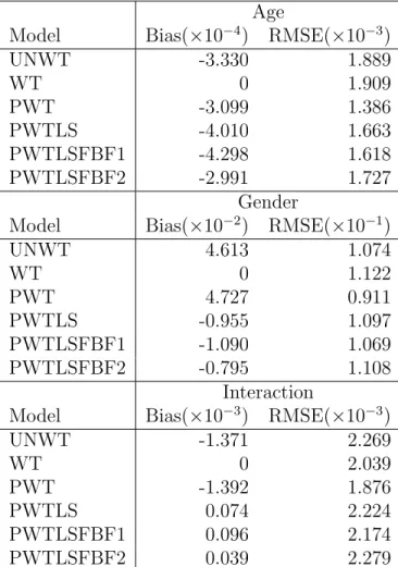
adjust-Age

Model Bias(×10−4₎ _RMSE(×10−3₎

UNWT -3.330 1.889 WT 0 1.909 PWT -3.099 1.386 PWTLS -4.010 1.663 PWTLSFBF1 -4.298 1.618 PWTLSFBF2 -2.991 1.727 Gender

UNWT 4.613 1.074 WT 0 1.122 PWT 4.727 0.911 PWTLS -0.955 1.097 PWTLSFBF1 -1.090 1.069 PWTLSFBF2 -0.795 1.108 Interaction

UNWT -1.371 2.269 WT 0 2.039 PWT -1.392 1.876 PWTLS 0.074 2.224 PWTLSFBF1 0.096 2.174 PWTLSFBF2 0.039 2.279

Table 2.9: Bias and RMSE for linear slope estimated for age, gender and interaction: unweighted, fully weighted, standard weight pooling estimator, and linear spline weight pooling estimator (without and with fractional Bayes Factor priors).Units present in parenthesis.

(45)

ment or poststratification may reduce variance as well as bias, but this is often not the case in practice. This variance inflation could be countered by a prediction esti-mation process that accounts for the unequal probability of selection. First a mean structure for sampled observationsy is proposed, such as a linear combination includ-ing another covariate Xβ. Then one could fit the proposed model, draw parameters from their estimated distributions, or posterior distributions in case under a Bayesian framework, and create the predicted y based on drawn parameters. Generating a posterior predi