Model-based analysis in survey: an application in analytic inference and a simulation in Small Area Estimation

Creative Components Iowa State University Capstones, Theses and _{Dissertations}

Summer 2019

Model-based analysis in survey: an application in analytic

Model-based analysis in survey: an application in analytic

inference and a simulation in Small Area Estimation

inference and a simulation in Small Area Estimation

[email protected]

Follow this and additional works at: https://lib.dr.iastate.edu/creativecomponents

Part of the Agricultural and Resource Economics Commons, Social Statistics Commons, and the

Statistical Models Commons

Recommended Citation Recommended Citation

Chen, Zhenzhen, "Model-based analysis in survey: an application in analytic inference and a simulation in Small Area Estimation" (2019). Creative Components. 301.

https://lib.dr.iastate.edu/creativecomponents/301

This Creative Component is brought to you for free and open access by the Iowa State University Capstones, Theses and Dissertations at Iowa State University Digital Repository. It has been accepted for inclusion in Creative Components by an authorized administrator of Iowa State University Digital Repository. For more information, please contact [email protected].

Model-based analysis in survey: an

application in analytic inference and a

simulation in Small Area Estimation

Zhenzhen Chen

Supervisor: Dr. Emily Berg

A thesis submitted to the graduate faculty

in partial fulfillment of the requirements for the degress of MASTER OF SCIENCE Major: Statistics Program of Committee: Dr. Emily Berg Dr. Daniel Nordman Dr. Cindy Yu

Iowa State University Ames, Iowa

Contents

Contents

1 Overview 1

1.1 Introduction . . . 1

1.2 The National Agricultural Workers Survey . . . 1

1.3 Small Area Estimation . . . 2

2 The National Agricultural Workers Survey Data 3 2.1 Background . . . 3

2.1.1 Farm Labor Suvery . . . 4

2.1.1.1 The NAWS Data . . . 4

2.1.1.2 Survey Weight . . . 5

2.1.2 Weights in Model-based Analysis for Survey Data . . . 6

2.2 Model for NAWS Data . . . 7

2.2.1 Basic Model from the NAWS Data . . . 8

2.2.1.1 The Lumley and Scott AIC Criterion . . . 9

2.2.1.2 Basic Model with Incorporating Weight . . . 10

2.2.2 Evaluation of Weights . . . 11

2.2.2.1 Comparison of Weighted Likelihood to Equal Weights . . . 11

2.2.2.2 Smooth Weight . . . 13

2.2.3 NAWS Data Application for Smooth Weight . . . 14

2.3 Conclusions . . . 16

3 Small Area Estimation 18 3.1 Introduction . . . 18

3.2 Model and Estimators . . . 18

3.3 Properties of Small Area Estimators . . . 20

3.4 Initial Model and Simulation Outline . . . 21

3.5 Conclusion . . . 26

References

Acknowledgements Appendix

List of Figures

List of Figures

A.1 Illustration of the difference between the distribution of the sample and the population for simulated example 1. Black dots: full population. Red dots: sampled elements. Black line: population regression line. Red line: least squares regression line based on the sample. . . . A.2 Illustration of the difference between the distribution of the sample and the

population for simulated example 2. Black dots: full population. Red dots: sampled elements. Black line: population regression line. Red line: least squares regression line based on the sample. . . .

List of Tables

List of Tables

2.1 Number of Workers Interviewed . . . 5

2.2 NAWS Variables (Numerical Variables) . . . 7

2.3 NAWS Variables (Categorical Variables) . . . 8

2.4 Variable Selection based on Augmented Model . . . 11

2.5 Weighting Approach for Variable Selection - Survey Weight . . . 12

2.6 Weighting approach for variable selection - sample weight vs. equal weight . . . . 13

2.7 Variable Selection based on weighting approach - sample weight, equal weight, and smooth weight . . . 14

2.8 Weighting approach for Variable Selection - Smoothed weight . . . 15

3.1 Comparison of Area level and Unit level Estimator - eij ∼N(0,1) . . . 22

3.2 Comparison of Area level and Unit level Estimator - eij ∼N(0,1) . . . 22

3.3 Comparison of Area level and Unit level Estimator - eij ∼N(0,1) . . . 23

3.4 Comparison of Area level and Unit level Estimator - eij ∼N(0,1),eij ∼ χ2 5−5 √ 10 . . 24

3.5 Comparison of Area level and Unit level Estimator - eij ∼N(0,1),eij ∼ √T5 5/3 . . 25

3.6 Comparison of Area level and Unit level Estimator - eij ∼N(0,1),eij ∼ χ2 3−3 √ 6 . . 26

1

1

Overview

1.1

Introduction

Traditional survey analyses use based inference. The source of randomness in design-based inference is the conceptual process of drawing repeated probability samples from a fixed finite population. based inference is based on the probability sampling design. Design-based inference procedures do not require an assumed satisfied model for the population or for the sample.

Model-based procedure play an important role in many types of survey data analysis. Unlike design-based methods, model-based procedures derive their statistical properties from an assumed model. In surveys, model-based procedures have an important role in nonresponse adjustment, small area estimation, and analytic inference. (In analytic studies, the goal is inference for the parameters of a statistical model defining a relationship between a response variable and an identified set of covariates.)

This creative component investigates the role of model-based procedures in surveys through a data analysis and a simulation study. The data analysis in chapter 2 is an example of analytic inference. The simulation study in chapter 3 pertains to small area estimation.

1.2

The National Agricultural Workers Survey

The object of the data analysis in Chapter 2 is to study the association between farm worker tenure (the number of years that a farm worker is employed with his/her current employer) and several characteristics of the farm worker. The data are from a complex, national survey called the National Agricultural Workers Survey (NAWS). The NAWS data we analyzed consist of 24 covariates, one survey weight and a file with 80 replicate weights for variance estimation provided by the U.S. Department of Labor (DOL).

We are using a step-wise variable selection method based on the AIC criteria to select one "best" model in the end. In the NAWS data, the survey weight accounts for unequal selection probabilities and nonresponses. An analysis that ignores the unequal selection probability can result in biased estimates of model parameters. Appropriately incorporating the survey weights is important in our research to correct bias and produce estimators with adequate statistical properties.

1.3 Small Area Estimation 2 Weighting and augmented modeling are the two methods to incorporate the weights. For the augmented modeling approach, the survey weight has been treated as one explanatory variable in the variable selection, so the error in the augmented model no longer correlates with survey weight. However, as can be seen, the survey weight does not have any significant meaning in the model. For the weighting approach, a weighted sum is substituted for the unweighted sum defining the score equation, where the weights are the survey weights. The restriction in the weighting approach is that variance in the weights can increase the variance of the estimators. One way to deal with this problem of variance inflation is to smooth the weight. In our study, we are going to discuss these issues associated with both the weighting and augmented approaches for the NAWS data.

1.3

Small Area Estimation

Small Area Estimation (SAE) is a method of gathering sufficient reliable estimates for a particular geographic area that does not provide enough information to get reliable estimates. SAE uses two types of models; unit-level models and area-level models.

The goal of the research study in Chapter 3 is to give a set of properties to consider when deciding whether to pursue a unit-level or area-level approach. We conducted a simulation to compare the mean spared error (MSE) of the five area-level and one unit-level estimators. The estimators we considered for the area-level model are 1). the direct estimator from the sample mean, 2). the direct estimator from a separate regression estimator, and 3) the direct estimator constructed with weights defined by the regression estimator for the overall population mean. The unit-level estimator uses the EBLUP for the unit-level model.

We considered six scenarios in this study. In addition to changing the random components from normal distribution to chi-square and t-distribution, we also vary the number of areas and the sample size of each area. From the results of this simulation study, the unit-level estimator performs the best. As the number of areas and the sample size of each area increases, the difference between the MSE of unit-level estimators and the MSE of area-level estimators constructed with the regression estimator shrink toward zero.

3

2

The National Agricultural Workers Survey Data

2.1

Background

In 2016, the topic of Labor in the Midwestern specialty cropping system has been analyzed by a graduate student, Anna Johnson, from the Iowa State University sociology department as a theses. The research used complex data from the National Agricultural Workers Survey (NAWS). NAWS is a national, random sample survey that collects data for more than fifty thousand farm workers. The questionnaire covers aspects including demographics, health, employment, and more. In her research, Johnson (2016) explores the association between the years that farm workers in the Midwest region have worked for their current employers with other characterizes related to the farm workers, such as their family income, education levels, and the years of farm work experience.

After reading and analyzing this paper, we identified three areas for improvement. Initially, we noticed that, in that paper, she set the years worked for current employers as the response variable (y), and intended to find out which covariates were good to fit the predictor. An

extensive literature review documented in Johnson (2016) suggested 28 possible covariates. The author included 24 out of the possible 28 covariates in the model. Secondly, the author used a log transformation for the response variable to stabilize the variances. Finally, the author used weighted estimating equation (Binder, 1983) to incorporate the survey weight, an approach that has been documented to inflate the standard survey for some variables Kim and Skinner (2013).

In our research, we will attempt to address areas of 1) covariate selection, 2) the response distribution and 3) the role of the weights. Specifically, for the first area, rather than using all potentially interesting covariates, we are going to select fewer covariables, leading to a smaller model. In principle, fewer variables will result in a more parsimonious and interpretable model and improve the precision of the estimators. For the second area, we are going to use the Poisson generalized linear model instead of using a log transformation for the response variable to stabilize the variances. The support of the dependent variable matches that of the Poisson distribution. Moreover, using the log transformation for the dependent variable will change the original dependent variable, which may make parameter interpretation difficult. For the last area, we will consider alternatives to incorporating the survey weight directly as a weight in the estimating equations with the aim of obtaining precise inferences without sacrificing statistical validity.

2.1 Background 4

2.1.1 Farm Labor Suvery

2.1.1.1 The NAWS Data

The National Agricultural Workers Survey is a national survey of United States farm workers, conducted by the United States Department of Labor (DOL) over the period 1989 to 2012. The survey population is composed of all the field workers active in crop agriculture in the continental United States. Based on the specific structure of agricultural production, the NAWS adopted a stratified multi-stage design to address seasonal and regional fluctuations in levels of farm work. Details of the sample design are available here: https://www.doleta.gov/naws/pages/methodology/ docs/NAWS_Statistical_Methods_AKA_Supporting_Statement_Part_B.pdf. We overview the

main aspects of the sampling design.

The strata are 12 regions divides a total of 497 Farm Labor Areas (FLAs) into 12 geographic strata. NAWS interviews are conducted in three interviewing cycles per year: February, June, and October. In each interviewing cycle, all 12 agricultural regions are included for the sample selection.

There are three sampling units. The primary sampling unit (PSU) is the FLA. Every year, the NAWS sample includes 90 out of the 479 FLAs. For each cycle, a sample of two to five FLAs will be selected using probabilities proportional to size (PPS) in each region. The second sampling unit is the county within an FLA. In an FLA, one county is usually selected using probabilities proportional to the size of the farm labor expenditures in that county during that interviewing cycle. Once the county has been sampled, all agricultural employers in that county will be listed. The process for selecting the employers uses restricted randomization, where a process of sorting the employers by zip code is used to improve the geographic spread of the sampled employers. Specifically, for each cycle and each county, 50 employers are randomly selected without replacement. If the requirement for the interview allocation has not been met, then another 50 employers are selected. The final level of the sampling unit is the farm laborers within employers. The workers have been sampled for each employer according to the restrictions shown in Table 2.1, which limit the burden of the survey process on the employer.

2.1 Background 5 Total Possible Interviewees Maximum interviewees per employer

5 - 25 5

26-40 8

41-75 10

≥75 12

Less than 5 All workers are to be interviewed

Table 2.1: Number of Workers Interviewed

2.1.1.2 Survey Weight

The complex NAWS design results in unequal probabilities of selection for different farm laborers. The survey weight accounts for unequal selection probabilities and non-response. In the data set, the composite survey weight used for analyzing the NAWS data is calledPWTYCRD.

It includes three weighting factors: sampling weights, non-response factors, and post-sampling adjustment factors.

The sampling weights reflect the stratified multi-stage sample design. Based on the design, one can calculate the probability of selecting an FLA, a county, a zip code, an employer and a worker. The selection probability is the product of the corresponding probability. The weight is the inverse of this selection probability. In the absence of nonresponse, the weight would allow unbaised estimation of population parameters.

The non-response weighting works to correct the deviation from the sampling method. For the NAWS data, the non-response adjustment is done at the region level, because the region is the smallest group in the NAWS survey with enough interviewees to calculate the size adjustment of the weight. If one region cannot provide enough information, then that region is combined with adjacent regions for weighting. The USDA Farm Labor Survey provides quarterly data at each region. The NAWS non-response adjustment modifies the weight to match official USDA estimates by region and season.

The role of the post-sampling weight is to allow the user to combine data from different cycles and different years in an analysis. We will use data for the Midwest region and for years 2009 to 2012. This subset is used in Johnson (2016) to represent the geographic and reference period of interest.

The NAWS data uses a cluster sampling strategy which has a stratified three-stage sample design including FLA, county, and farm workers. Based on the features the NAWS data sample design has, Fay’s balanced repeated replication (BRR) method was used to construct replicate

2.1 Background 6 weights for variance estimation. These replicate weights account for the fact that the sample is a cluster sample. Typically, the variance for cluster samples exceeds variances for simple random samples of the same sample sizes. In this case, Fay’s BRR method is going to be utilized to compensate for the larger variance. The DOL provides a new dataset including 80 replicate weights for variance estimation, which was used for the NAWS data analysis.

2.1.2 Weights in Model-based Analysis for Survey Data

The weights described in Section 2.1.1.2 account for unequal selection probabilities and nonresponse. An analysis that ignores the unequal selection probability can result in biased estimators of model parameters. In particular, in a regression model, if the error is correlated with the survey weight, estimators of regression parameters that ignore the weights are biased. Appropriately incorporating the survey weights can correct the bias and produce estimators with adequate statistical properties, such as consistency and unbiasedness. When the weight is corrected with the model error, we say that the sampling design is informative for the model. The concept of informative sampling is subtle, and we provide a more thorough descussion of this concept in the appendix to check.

Two approaches to incorporating the weights are often called “weighting” and “augmented modeling.” To explain the approach called “weighting,” recall that the maximum likelihood estimator is a root of the score equation, where the score equation is an unweighted sum of appropriately defined variables. For the “weighting” approach, the unweighted sum defining the score equation is replaced by a weighted sum, where the weights are the survey weights defined in Section 1.1.2. For the “augmented model” approach, the survey weights are included as an additional explanatory variable in the model. The theoretical motivation for the augmented model approach is that after including the weight as an explanatory variable, the error in the augmented model no longer correlates with the survey weight.

Both the “weighting” and “augmented model” approaches introduce challenges for the NAWS data. Model selection with the augmented model approach is straightforward to implement with existing software. The augmented model approach is not appealing for this application because the weight does not have a scientific meaning. Simultaneously, a limitation of the weighting approach is that variation in the weights can increase the variance of the estimator. One way to reduce variance inflation resulting from the weight is to smooth the weights. Weight smoothing techniques are discussed by Kim and Skinner (2013). We will discuss these issues associated with both the “weighting” and “augmented model” approaches in our analysis.

2.2 Model for NAWS Data 7

2.2

Model for NAWS Data

Following Johnson (2016), we focus on NAWS data for the Midwest region collected between 2009 and 2012. The Midwest region includes Illinois, Indiana, Iowa, Kansas, Missouri, Michigan, Minnesota, Nebraska, North Dakota, Ohio, South Dakota, and Wisconsin. The data set we have used is composed of 626 cases, 27 variables, and one weight. The objective is to understand relationships between the length of time that a farm worker remains at a farm job and characteristics of the farm worker. Because a large number of farm worker characteristics exist, we have used variable selection.

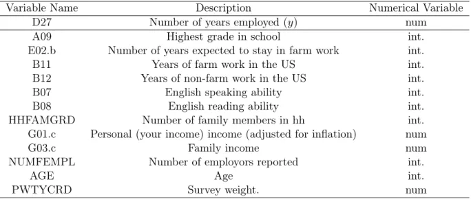
Table 2.2 and 2.3 consists the full set of covariates of interest. The response variabley is the

number of years that a farm worker has been employed with his/her current employer (D27). We choose the Poisson distribution because the support of the Poisson distribution is the set of integers. Furthermore, the analysis of Johnson (2016) showed a positive association between mean and the variance of the dependent variable (D27). After analysis of each original covariate from Table 2.2 and 2.3, there are 16 covariates treated as factor variables and 13 covariates as numeric variables. The survey weight PWTYCRD calculated in section 1.1.2 is used to analyze this NAWS data.

Variable Name Description Numerical Variable

D27 Number of years employed (y) num

A09 Highest grade in school int.

E02.b Number of years expected to stay in farm work int.

B11 Years of farm work in the US int.

B12 Years of non-farm work in the US int.

B07 English speaking ability int.

B08 English reading ability int.

HHFAMGRD Number of family members in hh int.

G01.c Personal (your income) income (adjusted for inflation) num

G03.c Family income num

NUMFEMPL Number of employors reported int.

AGE Age int.

PWTYCRD Survey weight. num

2.2 Model for NAWS Data 8

Variable Name Description Variable Levels

B03sum.b Num. adult education courses completed 0-No hour; 1-Yes_{3-No Answer} E04.b Ability to get a non-US farm job 0-No; 1-Yes_{7-Don’t Know} Accomp.b Accompanied with family 0-No_1-Yes

D30.b The way of the job was acquired

1-Self;4-Grower hires

5-Contractor hires;8-other refers 6-Employment refer

7-Welfare refers

9-labor union refers; 97-Other D11.b Paid Structure 1-By hour; 2-By piece_{3-Combination; 4-Salary} D20.b Other Bonuses 0-No; 1-Yes-grower_{7-Don’t know}

CROP.b Other Bonuses 1-Field Crops; 2-Fruit/Nuts;3-Horticulture; 4-Vege 5-Misc/Mult

D28.c Seasonal or year-round work 0- Year-round Work_{1-Seasonal Work}

TASK.b Type of Task 1-Pre-harvest; 2-Harvest_{3-Post-harvest; 4- Semi-skilled} Worktype.b Type of Work 1-Field; 1-Nursery_{3-Packing House; 7-Other}

NQ01.b Use of U.S. health care 0-No_1-Yes

NQ10sum.b Num. difficulties in obtaining health care 0-No; 1-Yes_{3-Don’t know} Indigenous.b Indigenous status 0-No Indigenous_{1- Indigenous}

A07 Birth Place 1-U.S.; 2-Mexico_3-Other

MIGTYPE2.b Migrant Type Settled; Follow the Crop_{Shuttle; Newcomer}

GENDER.b Gender 0-Male_1-Female

currstat.c Documentation Status 1-Citizen_{4-Unauthorized}

Table 2.3: NAWS Variables (Categorical Variables)

2.2.1 Basic Model from the NAWS Data

The first question we address is how incorporating the weights impacts the model selection process. To start, we can compare results of model selection using the standard AIC criterion for simple random samples. We begin with a full model and proceed in a step-wise process, dropping

2.2 Model for NAWS Data 9 insignificant variables or groups of insignificant variables.

2.2.1.1 The Lumley and Scott AIC Criterion

Lumley and Scott (2015) adapt the AIC criterion to a complex survey framework. Their AIC criterion is of the form

dAIC =−2n`w(ˆθ) + 2pδ,ˆ¯ (2.1)

where nis the sample size,`w(ˆθ) is a weighted log likelihood, andˆ¯δ is an estimated design effect.

The criterion dAIC modifies the penalty in the usual AIC criterion by the multiplier ˆ¯δ. If δˆ¯= 1, then the penalty indAIC simplifies to the usual AIC penalty for a simple random sample.

The design effect measures the effect of the sample design on the variances of estimators. For a multi-dimensional parameter vector (such as the vector of regression coefficients) the design effect is

¯

δ =trace([VSRS(ˆθ)]−1VDes(ˆθ))/p, (2.2)

whereVSRS(ˆθ)andVDes(ˆθ) are the covariance matrices of the estimatorθˆfor the simple random

sample and the designDes, respectively. Additionally,p is the dimension of θ. An estimated

design effect _δˆ¯_{is defined by estimating the covariance matrices in (2.2).}

The design effect depends on the nature of the sample design. For simple random samples, an efficient stratification will decrease the design effects. However, clustering typically increases the design effect, since the units in the same cluster are typically more similar to each other than units in different clusters. Clustering also decreases the effective sample size, and increases the variances of estimators relative to simple random samples.

Because of the complex design of the NAWS survey, we hesitated to use the AIC criterion approach for a simple random sample. The NAWS design includes several stages of clustering (farm labor areas, counties, and employers). If farm workers within a cluster are more similar to each other than farm workers in different clusters, then the effective sample size is smaller than n, and the design effect exceeds 1. In a preliminary analysis, we implemented step-wise

variable selection, using the AIC criterion approach for a simple random sample. We found that a relatively large model was selected and that coefficients for many of the variables in the selected model were no longer judged “statistically significant” after accounting for the effect of the design

2.2 Model for NAWS Data 10 in the estimation and variance estimation procedures. For the purpose of interpretation, a more parsimonious model seems desirable.

We had difficulty implementing model selection with the exact Lumley and Scott (2015) AIC criterion using R. We define a simplification to Lumley and Scott (2015) AIC procedure for use

in variable selection.

We define an estimated design effect for the full model by ˆ

¯

δf ull =trace([ ˆVSRS(ˆθf ull)]−1VˆDes(ˆθf ull))/pf ull, (2.3)

where pf ull is the dimension of the vector of regression coefficients,θˆf ull, for the full model. We

then apply usual step-wise model selection using_δˆ¯_{f ull2p as the penalty in thedAIC criterion.} The estimated design effect for the full model, including the weight as a covariate, is approximately 5.0. The penalty for the Lumley and Scott (2015) AIC criterion would then be 2pf ull5 = 10pf ull for the full model. On this basis, we use the step-wise AIC procedure

implemented in theR function stepAIC withk= 10to implement variable selection.

2.2.1.2 Basic Model with Incorporating Weight

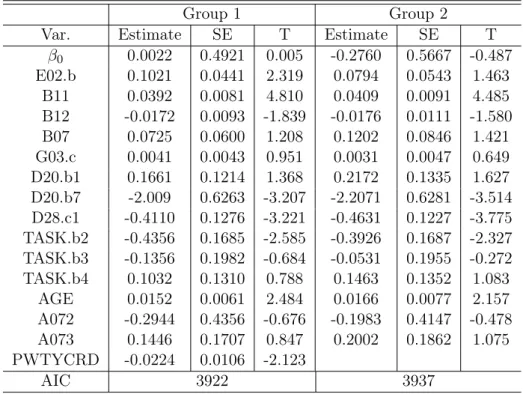
The augmented model approach has been applied to incorporating weight. The U.S. Department of Labor (DOL) provides a weight called PWTYCRD which can be used as an explanatory variable and applied to the model selection. Additionally, for dealing with stratified sampling problems, the DOL has constructed 80 replicate weights for variance estimates by using Fay’s method of Balanced Repeated Replication. We used “group 1” to indicate all 24 covariates, including PWTYCRD, and “group 2” to indicate 23 covariates, not including PWTYCRD. For using the AIC criterion discussed in section 2.2.1.1, we selected the two "best" models for each group.

Table 2.4 shows the kinds of variables and statistics we have included in both models. Firstly, for using the step-wise process, we can see that PWTYCRD as an explanatory variable has been selected in the "best" model. Secondly, the model with PWTYCRD has a smaller standard error for each variable than the standard error value in the model excluding PWTYCRD. Finally, compared with the AIC value for the model without weight as an explanatory variable, we can see that the model with weight has a smaller AIC value. As discussed above, we can conclude that the weight has a significant effect on model selection, and it also reduces the standard error for each variable for the NAWS data. This illustrates the meaning of the term "informative sampling":

2.2 Model for NAWS Data 11 the weight contains information about the error in the model that omits the weight. We work that the standard error in Table 2.4 may be optimistic because we have not get incorporating the replicate weight. In the next section, we will use the replicate weights for variance estimation.

Group 1 Group 2

Var. Estimate SE T Estimate SE T

β0 0.0022 0.4921 0.005 -0.2760 0.5667 -0.487 E02.b 0.1021 0.0441 2.319 0.0794 0.0543 1.463 B11 0.0392 0.0081 4.810 0.0409 0.0091 4.485 B12 -0.0172 0.0093 -1.839 -0.0176 0.0111 -1.580 B07 0.0725 0.0600 1.208 0.1202 0.0846 1.421 G03.c 0.0041 0.0043 0.951 0.0031 0.0047 0.649 D20.b1 0.1661 0.1214 1.368 0.2172 0.1335 1.627 D20.b7 -2.009 0.6263 -3.207 -2.2071 0.6281 -3.514 D28.c1 -0.4110 0.1276 -3.221 -0.4631 0.1227 -3.775 TASK.b2 -0.4356 0.1685 -2.585 -0.3926 0.1687 -2.327 TASK.b3 -0.1356 0.1982 -0.684 -0.0531 0.1955 -0.272 TASK.b4 0.1032 0.1310 0.788 0.1463 0.1352 1.083 AGE 0.0152 0.0061 2.484 0.0166 0.0077 2.157 A072 -0.2944 0.4356 -0.676 -0.1983 0.4147 -0.478 A073 0.1446 0.1707 0.847 0.2002 0.1862 1.075 PWTYCRD -0.0224 0.0106 -2.123 AIC 3922 3937

Table 2.4: Variable Selection based on Augmented Model

2.2.2 Evaluation of Weights

2.2.2.1 Comparison of Weighted Likelihood to Equal Weights

We saw in Section 2.2.1.1 that the survey weight appears to be a significant predictor. Incorporating the weights in some fashion seems necessary to obtain valid statistical inferences. As discussed, the augmented model approach is not ideal because the weight is not scientifically meaningful in this context. A natural alternative is to consider the “weighting” approach, where the survey weights are used as weights in the estimation procedure. In this section, we compare the estimates and standard errors for using the weighting approach. We first use the raw survey weight, then use equal weights. Additionally, we use replicate variance estimates for both the "survey weight" and "equal weight" procedures in this section.

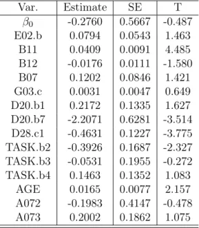
Based on Table 2.5, when using the weighting approach for the survey weight, we found that only a few variables are typical "statistically significant": B11 (years of farm work in the US), D20.b7 (other bonuses, don’t know), D28.c1 (seasonal work), TASK.b2 (Harvest), and AGE (age). From using the step-wise process, the insignificant covariates should be dropped, yet few

2.2 Model for NAWS Data 12 significant covariates remain after this process. We, therefore, construct an equal weight that is formulated by the mean of PWTYCRD to assess the effect of variation in PWTYCRD on the standard error. Var. Estimate SE T β0 -0.2760 0.5667 -0.487 E02.b 0.0794 0.0543 1.463 B11 0.0409 0.0091 4.485 B12 -0.0176 0.0111 -1.580 B07 0.1202 0.0846 1.421 G03.c 0.0031 0.0047 0.649 D20.b1 0.2172 0.1335 1.627 D20.b7 -2.2071 0.6281 -3.514 D28.c1 -0.4631 0.1227 -3.775 TASK.b2 -0.3926 0.1687 -2.327 TASK.b3 -0.0531 0.1955 -0.272 TASK.b4 0.1463 0.1352 1.083 AGE 0.0165 0.0077 2.157 A072 -0.1983 0.4147 -0.478 A073 0.2002 0.1862 1.075

Table 2.5: Weighting Approach for Variable Selection - Survey Weight

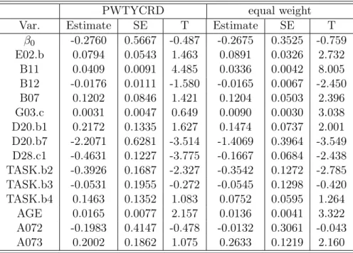
Table 2.6 shows a comparison between PWTYCRD and equal weight based on the weighting approach. From the table, it can be seen that using equal weight reduces the SE of each covariate and more variables become statistically significant. Those significant covariates are E02.b (number of the years expected to stay in farm work), B11 (years of farm work in the US), B12 (years of non-farm work in the US), B07 (English speaking ability), G03.c (family income), D20.b1 (having other bonuses), D20.b7 (don’t know if having other bonuses), D28.c1 (seasonal work), TASK.b2 (harvest), AGE (age), and A073 (birth place, other place). As can be seen that, only three covariates do not significant predicate the dependent variables. When checking the estimates for each covariates, the direction of the each covariate are the some for both weights. After using equal weights, the estimates of covariates G03.c (family income) grows. However, the estimates of covarites D28.c1 (season work), TASK.b4 (semi-skilled), and A072 (birth place: Mexico) shrinks extremely. Using equal weights reduces the design effect but may omit important information.

2.2 Model for NAWS Data 13

PWTYCRD equal weight

Var. Estimate SE T Estimate SE T

β0 -0.2760 0.5667 -0.487 -0.2675 0.3525 -0.759 E02.b 0.0794 0.0543 1.463 0.0891 0.0326 2.732 B11 0.0409 0.0091 4.485 0.0336 0.0042 8.005 B12 -0.0176 0.0111 -1.580 -0.0165 0.0067 -2.450 B07 0.1202 0.0846 1.421 0.1204 0.0503 2.396 G03.c 0.0031 0.0047 0.649 0.0090 0.0030 3.038 D20.b1 0.2172 0.1335 1.627 0.1474 0.0737 2.001 D20.b7 -2.2071 0.6281 -3.514 -1.4069 0.3964 -3.549 D28.c1 -0.4631 0.1227 -3.775 -0.1667 0.0684 -2.438 TASK.b2 -0.3926 0.1687 -2.327 -0.3542 0.1272 -2.785 TASK.b3 -0.0531 0.1955 -0.272 -0.0545 0.1298 -0.420 TASK.b4 0.1463 0.1352 1.083 0.0752 0.0595 1.264 AGE 0.0165 0.0077 2.157 0.0136 0.0041 3.322 A072 -0.1983 0.4147 -0.478 -0.0132 0.3061 -0.043 A073 0.2002 0.1862 1.075 0.2633 0.1219 2.160

Table 2.6: Weighting approach for variable selection - sample weight vs. equal weight

2.2.2.2 Smooth Weight

One can obtain a compromise between the estimators based on the survey weights and equal weights if one can specify a model for the weights. Modeling the weights is sometimes called weight smoothing. In this section, we consider a particular weight smoothing procedure discussed by Kim and Skinner (2013).

By Kim and Skinner (2013), the smoothed weight is defined asde_i= Es(di

|xi,yi)

Es(di|xi) , where di is PWTYCRD.

The correspondingβe_{SP S} can be expressed as the solution to

e USP S(β) = N X i=1 Ii Es(di|xi, yi) Es(di|xi) (yi−x 0 iβ)xi = 0, (2.4)

where Es(di|xi, yi) = E(di|xi, yi, Ii = 1), and Es(di|xi) = E(di|xi, Ii = 1). We use the same

covariates selected though the stepwise procedure (Table 2.3) in the model for the weight. Table 2.7 presents the estimates, standard errors and t statistics constructed with the smoothed weight, and compares with the other two weights. From the table, smoothing the weight reduces the standard error, relative to the use of the original weights. The t statistics for most covariates have doubled the value for using smooth weight. Those covaraites are E02.b (num.of years

2.2 Model for NAWS Data 14 expected to stay in the farm work), B11 (years of farm work in the US), B07 (English speaking ability), G03.c (family income), TASK.b3 (post-harvest), A073 (other birth place). Specifically speaking, the t statistic of covariate family income increases from 0.0649 to 2.924, and the estimates coefficient grows form 0.0031 to 0.0088 after using smooth weight. When we compare equal weight and smoothed weight, the value of SEs and t statistics of majority variables between these two weights do not have a big difference, that means these two weights selected almost the same covariates in the final model. Additionally, it can also be seen that the estimates for each covariate having the same direction for all three weights.

PWTYCRD Equal Weight Smooth Weight

Var. Estimate SE T Estimate SE T Estimate SE T

β0 -0.2760 0.5667 -0.487 -0.2675 0.3525 -0.759 -0.3074 0.3570 -0.861 E02.b 0.0794 0.0543 1.463 0.0891 0.0326 2.732 0.0899 0.0323 2.784 B11 0.0409 0.0091 4.485 0.0336 0.0042 8.005 0.0330 0.0042 7.775 B12 -0.0176 0.0111 -1.580 -0.0165 0.0067 -2.450 -0.0163 0.0068 -2.391 B07 0.1202 0.0846 1.421 0.1204 0.0503 2.396 0.1260 0.0509 2.474 G03.c 0.0031 0.0047 0.649 0.0090 0.0030 3.038 0.0088 0.0030 2.924 D20.b1 0.2172 0.1335 1.627 0.1474 0.0737 2.001 0.1594 0.0752 2.119 D20.b7 -2.2071 0.6281 -3.514 -1.4069 0.3964 -3.549 -1.4186 0.3941 -3.600 D28.c1 -0.4631 0.1227 -3.775 -0.1667 0.0684 -2.438 -0.1668 0.0696 -2.398 TASK.b2 -0.3926 0.1687 -2.327 -0.3542 0.1272 -2.785 -0.3579 0.1288 -2.779 TASK.b3 -0.0531 0.1955 -0.272 -0.0545 0.1298 -0.420 -0.0551 0.1323 -0.416 TASK.b4 0.1463 0.1352 1.083 0.0752 0.0595 1.264 0.0786 0.0627 1.254 AGE 0.0165 0.0077 2.157 0.0136 0.0041 3.322 0.0137 0.0042 3.244 A072 -0.1983 0.4147 -0.478 -0.0132 0.3061 -0.043 -0.0035 0.3085 -0.012 A073 0.2002 0.1862 1.075 0.2633 0.1219 2.160 0.2727 0.1246 2.189

Table 2.7: Variable Selection based on weighting approach - sample weight, equal weight, and

smooth weight

2.2.3 NAWS Data Application for Smooth Weight

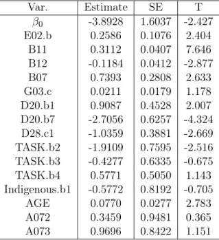
Based on what we have discussed in section 2.2. We are going to use smoothed weight in NAWS data. The following table shows the covariates it selected and corresponding statistics each variable has. For the smooth weight, we repeat the step-wise AIC procedure implemented in theR function stepAICwith k= 8 to implement variable selection.

2.2 Model for NAWS Data 15 Var. Estimate SE T β0 -3.8928 1.6037 -2.427 E02.b 0.2586 0.1076 2.404 B11 0.3112 0.0407 7.646 B12 -0.1184 0.0412 -2.877 B07 0.7393 0.2808 2.633 G03.c 0.0211 0.0179 1.178 D20.b1 0.9087 0.4528 2.007 D20.b7 -2.7056 0.6257 -4.324 D28.c1 -1.0359 0.3881 -2.669 TASK.b2 -1.9109 0.7595 -2.516 TASK.b3 -0.4277 0.6335 -0.675 TASK.b4 0.5771 0.5050 1.143 Indigenous.b1 -0.5772 0.8192 -0.705 AGE 0.0770 0.0277 2.783 A072 0.3459 0.9481 0.365 A073 0.9696 0.8422 1.151

Table 2.8: Weighting approach for Variable Selection - Smoothed weight

Table 2.8 for using smoothed weight for weighting approach, the covariates selected in the final model and its corresponding estimates, standard error, and t statistics. The covariates have been selected in the final model for using step-wise are totally 10 covariates. They are E02.b (number of years expected to stay in farm work), B11 (years of farm work in the US), B12 (years of non-farm work in the US), B07 (English speaking ability), G03.c (family income), D20.b1 (no other bonuses), D20.b7 (don’t know if having other bonuses), D28.c1 (seasonal work), TASK.b2 (harvest), TASK.b3 (post-harvest), TASK.b4 (semi-skilled), Indigenous.b1 (has indigenous status), AGE (age), A072 (birth place: Mexico), and A073 (birth place: other). These ten covariates can separate in three different areas: human and social capital, the context of reception - employer, and control.

For the concept of human and social capital, four independent variables have been selected to the final model. These are E02.b (number of years expected to stay in farm work), B11 (years of farm work in the US), B12 (years of non-farm work in the US), and B07 (English speaking ability). All these four variables show statistically significant evidence for predicting the number of years employed. For the number of years expected to stay in farm work (E02.b), the range of the answer is between 1 year to 7 years, and most interviewees prefer to stay in 5 years. It shows a significant positive relationship between the number of years expected to stay in farm work and employed by their current employer. For years of farm work (B11) and non-farm work (B12), from the statistics listed in Table 2.8, we can see that number of years farm work have a positive relationship with years worked for the current farm work employer. It shows that the

2.3 Conclusions 16 more time you work on the farm work in the US, the more time you will stay working for the current employer. Non-farm work in the US shows a negative predictor of job tenure. The final covariate in this area is the English speaking ability. This covariate shows a positive relationship with job tenure.

The second area is the contexts of reception - employer. There are six covariates in this area, D20.b1 (no other bonuses), D20.b7 (don’t know if having other bonuses), D28.c1 (seasonal work), TASK.b2 (harvest), TASK.b3 (post-harvest), TASK.b4 (semi-skilled). All these six covariates discuss job structure. These six covariates talk about whether an employer will offer a bonus, whether employees work for seasonal round work, and what kind of task the employers will assign. When checking the t statistics form the Table 2.8, it can be seen that offering bonus, working for the seasonal-round and assigning the harvest task are significant predictors. In other words, these three aspects show a big effect for the number of years the farm workers stay in their current work.

The third area is control, that includes the variables: G03.c (family income), AGE (age), A072 (birth place: Mexico), A073 (birth place: other), and Indigenous.b1 (have indigenous status). Birth place and type of indigenous are both categorical variables, all the levels of these two covariates has been selected in to the model. However, only birth place from other places excluding US and Mexico (A073) is significant predictors for the job tenure. Age and family income are statistically significant predictors of the independent variable.

2.3

Conclusions

The aim of this study is finding the association between the number of years farm workers are employed in their current employer and farm worker characteristics. We do step-wise variable selection based on Lumley and Scott (2015) AIC criterion. Incorporating the survey weight leads to larger estimated variances. We thus turn to reformulate two weights and use the augmented model approach and the weighting approach. Based on the step-wise model selection method with a smoothed weight, ten covariates have been selected in our final model. These are years of farm work in the US, years of non-farm work in the US, English speaking ability, family income, whether they received other bonuses, work with employer in seasonal or year-round work, type of task, indigenous status, age, and birth place. That is one variable different from the variable selected based on the sample weight in Table 2.5. Using smoothed weight, the variable type of indigenous has been selected, but the model for the survey weight does not include this variable. When checking the t statistic of this variable in Table 2.7 we can found it is not a significant

2.3 Conclusions 17 predictor for job tenure.

For the future research, one implication can be work is we can find what the important factors that impact the weight. In our current research, we constructed a smoothed weight based on Kim and Skinner (2013). The covarites we selected to construct the smooth weight may not the best way to modeling the response variables.

18

3

Small Area Estimation

3.1

Introduction

When constructing small area estimates with unit level data, the analyst is faced with the decision of whether to pursue standard “unit-level” models (Battese et al., 1988) or “area-level” models (Fay and Herriot, 1979). We compare and contrast these two approaches. Our initial goal was to provide the analyst with a set of properties to consider when deciding whether to pursue a unit-level or area-level approach. Our conjecture was that using an area-level model, with an appropriately defined direct estimator, may be nearly as efficient as the unit-level estimator for large m and ni when the model is correctly specified and may be more robust to model

mis-specification. For this research, we narrow our original scope and focus on the distributions of the area effects and unit level errors in the unit level model. We compare area-level estimators based on a regression estimator to area-level estimators based on a Horvitz-Thompson estimator. We study the properties of alternative estimators through simulation and through analytical derivations.

Hidiroglou and You (2016) also compare area level models and unit-level models. They focus on the case of an informative sample design. The three area level estimators are the unweighted sample mean, the Horvitz-Thompson estimator, and the Hajek estimator.

Our work extends Hidiroglou and You (2016) and Namazi-Rad and Steel (2015). We include a regression estimator among the area level estimators, which has not been considered previously. We focus on a particular form of mis-specification of the unit-level model, where the error distributions are not normal distributions.

3.2

Model and Estimators

yij =β0+β1xij +bi+eij, i= 1, . . . , D;j= 1, . . . , Ni, (3.1)

where xij ∼ (0, σx2), bi ∼(0, σb2),eij ∼(0, σ2e), and the notation X ∼ (A, B) means that X is

a random variable with meanA and variance B. We assume that a stratified simple random

3.2 Model and Estimators 19 finite population area level means defined by

¯ yNi =N −1 i Ni X j=1 yij. (3.2)

We consider predictors of (3.2), defined as follows:

1. First, we consider an estimator for an area-level model where the direct estimator is the sample mean y¯ni =n

−1

i

Pni

j=1yij. Define the area-level model by

¯

yni =β0+β1x¯Ni+bi+ηi, (3.3) where ηi ∼(0,(σx2+σe2)/ni). LetθˆiBLU P,1 denote the typical area level predictor based on

(3.3).

2. The second estimator is an estimator for an area-level model where the direct estimator is a separate regression estimator; that is, a regression estimator where the regression variables are interactions between the covariatexij and area level indicator variables. To compute

the regression estimator, let the weight for elementj in areai be defined by w_ijreg1 = 1 ni + (¯xNi−x¯ni) Pni j=1(xij −x¯ni)2 (xij−x¯ni).

Define the direct estimator for areaiby

ˆ yi,reg1= ni X j=1 wreg_ij 1yij.

Then, we will specify the area-level model by ˆ yi,reg1 =β0+β1x¯Ni+bi+ ˜ηi, (3.4) whereη˜i ∼(0,(σ2e/ni+δi)), and δi=σ2e(¯xNi−x¯ni) 2   ni X j=1 (xij −x¯ni) 2   −1

By properties of normal andχ2 _{distributions, E[δ}

i] =σe2(1−niNi−1)(ni(ni−3))−1.

3.3 Properties of Small Area Estimators 20 estimator for the overall population mean. Define the weight by

w_ijreg1 = 1 n+ (¯xN−x¯n) Pm i=1 Pni j=1(xij −x¯n)2 (xij −x¯n)

Define the direct estimator for areaiby

ˆ yi,reg2= Pni j=1w reg2 ij yij Pni j=1wij .

4. The EBLUP for the unit-level model (3.1).

3.3

Properties of Small Area Estimators

We consider the properties of the estimators under the assumption that the model parameters are known. Ignoring the finite population correction factor, the MSE of the BLUP ofy¯Ni is

E[(ˆy¯BLU P_Ni −y¯Ni) 2_{] =γ} iσe2n−1i , where γi= σ2_b σ2 b +σ2en−1i .

The MSE of the small area predictor for the model (3.3) based on the sample mean is given by

E[(ˆθBLU P,_i 1−θi)2] =γi,2(σ2x+σe2)/ni, where γi,2= σ2_b σ2_b + (σ2 x+σe2)/ni .

Asσ2_x→ ∞, γi,2(σ2x+σe2)/ni →σ2_b > γiσ2n−1_i , as expected. The MSE of the small area predictor

for the model (3.4) is

3.4 Initial Model and Simulation Outline 21 where γi,3 = σ2_b σ_b2+σ2 e/ni(1 + 1/(ni−3)) .

The difference between the MSE of the area level estimator constructed with the regression estimator and the MSE of the unit-level estimator is due to the additional termδi in the variance

of the regression estimator with expectation(ni(ni−3))−1. As ni→ ∞, the difference between

the MSE of_θˆBLU P,2

i and the MSE of the unit-level estimator approaches zero.

3.4

Initial Model and Simulation Outline

The analytically derivations of the MSEs of the estimators ignores the effect of parameter estimation. We conduct a simulation study to assess the effect of parameter estimation on the MSEs of the predictors. We will use the simulation framework from Sinha and Rao (2009) as a guideline. To start, we assumexij ∼N(0,1),bi ∼N(0,1), andeij ∼N(0,1). We then progress to

consider the cases in which the random component does not have normal distributions, differences in number of areas, and differences in the sample size of each area. The estimators considered in the simulation study are defined as follows:

• MSE1 – The MSE of the regression estimatoryˆi,reg1 • MSE2 – The MSE of the regression estimatoryˆi,reg2 • MSE3 – The MSE of the sample mean.

• MSE4 – The MSE of _θˆBLU P,2

i , the area-level EBLUP constructed with the regression

estimatoryˆi,reg1.

• MSE5 – The MSE of_θˆBLU P,1

i , the area-level EBLUP constructed with sample mean.

• MSE6 – The MSE of the EBLUP for the unit-level model.

Scenario I: We generatem= 40areas withNi= 40 for 20 areas, andNi = 120for 20 areas.

A stratified sample is selected with areas as strata with ni = 0.1Ni. We assumexij ∼N(0,1),

3.4 Initial Model and Simulation Outline 22

Type Estimator n = 4 n =12_{MSE MSE} Area level MSE 1 0.4520 0.0830 MSE 2 0.4482 0.1466 MSE 3 0.4505 0.1492 MSE 4 0.2697 0.0775 MSE 5 0.3276 0.1328 Unit level MSE 6 0.1879 0.0704

Table 3.1: Comparison of Area level and Unit level Estimator - eij ∼N(0,1)

Table 3.1 shows the comparison of the unit-level and area-level estimators for sample sizes

n= 4 andn= 12. From Table 1, when increasing the sample size fromn= 4to12, it can be seen that all estimators’ MSEs greatly shrink, especially for the area-level regression estimator (MSE1). Among all estimators, the EBLUP for the unit-level model (MSE6) has the smallest MSE for both sample sizes. Within the area-level, the EBLUP constructed with the regression estimator (MSE 4) has the smallest MSE for both sample sizes when compared with the other four estimators. Whenn= 4, the MSE 4 is 0.2967, that is almost half than the MSE 1 at 0.4520, but whenn= 12, there is no big difference between these two estimators. The MSE of area-level EBLUP constructed with sample mean (MSE5) has smaller values than the MSE of the sample size (MSE3) for both sample sizes. Additionally, when sample size grows, the difference between these two estimators shrinks. The results show that increasing the sample size in each area has big effects on reducing the MSE for each estimator. The unit-level estimator has a smaller MSE for both sample sizes. Moreover, the EBLUP estimator performs well for area-level and unit-level models when the sample size is smaller.

Scenario II: We generatem= 60 areas withNi = 40for the first 20 areas, Ni= 120 for the

next 20 areas, andNi = 360 for the last 20 ares. A stratified sample is selected with areas as

strata withni = 0.1Ni. We assumexij ∼N(0,1),bi∼N(0,1), and eij ∼N(0,1).

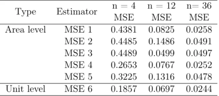
Type Estimator n = 4 n = 12 n= 36_{MSE MSE MSE} Area level MSE 1 0.4381 0.0825 0.0258 MSE 2 0.4485 0.1486 0.0491 MSE 3 0.4489 0.0499 0.0497 MSE 4 0.2653 0.0767 0.0252 MSE 5 0.3225 0.1316 0.0478 Unit level MSE 6 0.1857 0.0697 0.0244

Table 3.2: Comparison of Area level and Unit level Estimator - eij ∼N(0,1)

3.4 Initial Model and Simulation Outline 23

n = 4, n = 12, and n = 36. As the sample size increases for each area, the MSE for each estimator decreases, specifically for the MSE of the regression estimator (MSE1) and the MSE of the EBLUP with regression estimator (MSE4). The EBLUP for the unit-level model (MSE6) still has the smallest value for all estimators among all three sample sizes. In the area-level estimator, MSE4 has the smallest MSE among all sample sizes when compared with the other four estimators. As the sample size increases for each area, it can be seen that the difference between MSE4 and MSE6 becomes smaller. Moreover, the MSE value between MSE4 and MSE1 also grow closer. In summary, increasing the sample size for each area has a big effect in reducing the MSE for the regression estimator and the EBLUP with the regression estimator in area-level model.

Scenario III: We increase the sample areas from40areas to400areas, with 200areas with

Ni = 40, andNi= 120 for another200areas. A stratified sample is selected with areas as strata

withni = 0.1Ni. We assumexij ∼N(0,1),bi ∼N(0,1), and eij ∼N(0,1).

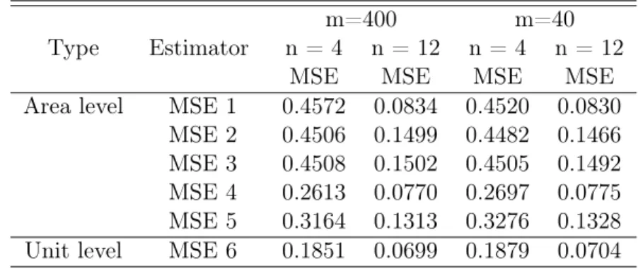
Type Estimator n = 4 n = 12 n = 4 n = 12m=400 m=40

MSE MSE MSE MSE

Area level MSE 1 0.4572 0.0834 0.4520 0.0830 MSE 2 0.4506 0.1499 0.4482 0.1466 MSE 3 0.4508 0.1502 0.4505 0.1492 MSE 4 0.2613 0.0770 0.2697 0.0775 MSE 5 0.3164 0.1313 0.3276 0.1328 Unit level MSE 6 0.1851 0.0699 0.1879 0.0704

Table 3.3: Comparison of Area level and Unit level Estimator - eij ∼N(0,1)

Table 3.3 shows the comparison between the unit-level and area-level models in a different number of areas. Increasing 40 to 400 areas, there is no big difference between each value for the same standard. The MSE value of the EBLUP of unit-level (MSE6) slightly shrinks from area 40 to area 400, that is 0.1879 shrinks to 0.1851 for sample sizen= 4 and 0.0704 decreases to 0.0699 for sample sizen= 12. The MSE of area-level EBLUP with the regression estimator (MSE4) also slightly decreases while the number of areas increase from 40 to 400, that is 0.2697 to 0.2613 for n= 4 and 0.0775 to 0.0770 forn= 12. In summary, increasing the number of the areas does not have much influence on reducing the MSE for each estimator. This shows us that the effect of parameters estimator on the variances of the predctors is small.

Based on the result from scenarios I to III, it can be concluded that the EBLUP for the unit-level model (MSE6) always has the smallest MSE no matter the number of areas or the sample size in each area. However, increasing the sample size for each area will make MSE of

3.4 Initial Model and Simulation Outline 24 the area-level EBLUP with regression (MSE4) grow closer to MSE6. Moreover, the EBLUP estimator will perform well under unit-level and area-level models when sample size in each area is small. We then consider the cases that change the random components from normal distribution to Chi-square distribution and t distribution.

Scenario IV: For the following sections, we are going to change the random component from Normal distribution to Chi-square distribution, and compare the MSE for each estimator. We generate m= 40 areas with Ni= 40for 20 areas and Ni = 120for 20 areas. A stratified sample

is selected with areas as strata with ni = 0.1Ni. We assume xij ∼ N(0,1), bi ∼N(0,1), and

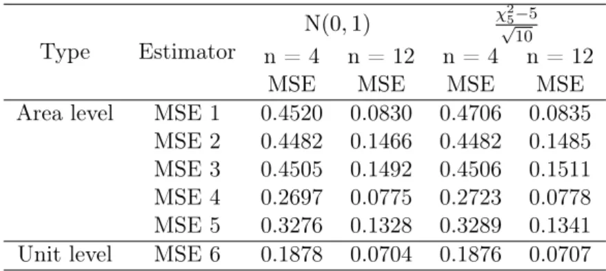
eij ∼ χ2 5−5 √ 10. Type Estimator N (0,1) χ_√25−5 10 n = 4 n = 12 n = 4 n = 12

MSE MSE MSE MSE

Area level MSE 1 0.4520 0.0830 0.4706 0.0835 MSE 2 0.4482 0.1466 0.4482 0.1485 MSE 3 0.4505 0.1492 0.4506 0.1511 MSE 4 0.2697 0.0775 0.2723 0.0778 MSE 5 0.3276 0.1328 0.3289 0.1341 Unit level MSE 6 0.1878 0.0704 0.1876 0.0707

Table 3.4: Comparison of Area level and Unit level Estimator - eij ∼N(0,1),eij ∼ χ2

5−5

√ 10

Table 3.4 shows the comparison between unit-level and area-level model for different random component distributions. It can be seen that using χ2 _{distribution, each value in the same} standard does not have a big difference with using a normal distribution for the random component. The area-level EBLUP with regression (MSE4) slightly grows for both sample sizes with the error term change the distribution from standard normal to χ2. Forn= 4, the MSE value increases from 0.2697 to 0.2723, and for n= 12, the number increase from 0.0775 to 0.0778. For the MSE of EBLUP in the unit-level (MSE 6) slightly drops for using Chi-square distribution for the error term. For the sample size is 4, the value is 0.1878, and the value is 0.1876 for Chi-square distribution with the random component. These difference are small, and we did not assess the Monte Carlo variance. For the sample size of 12, the MSE is from 0.0704 decreases to 0.0707 for Chi-square distribution with the random component. In summary, the random component with Chi-square distribution does not show influence in reducing the MSE values for each estimator. Scenario V: For the next sections, we are going to changing the random component from normal distribution to T distribution, and compare the MSE for the each estimator. We generate m= 40 areas withNi = 40for 20 areas andNi= 120for 20 areas. A stratified sample is selected

3.4 Initial Model and Simulation Outline 25 with areas as stata with ni= 0.1Ni. We assumexij ∼N(0,1),bi ∼N(0,1), andeij ∼ √T5

5/3.

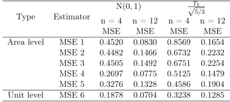
Type Estimator N

(0,1) √T5

5/3 n = 4 n = 12 n = 4 n = 12

MSE MSE MSE MSE

Area level MSE 1 0.4520 0.0830 0.8569 0.1654 MSE 2 0.4482 0.1466 0.6732 0.2232 MSE 3 0.4505 0.1492 0.6751 0.2254 MSE 4 0.2697 0.0775 0.5125 0.1479 MSE 5 0.3276 0.1328 0.4586 0.1904 Unit level MSE 6 0.1878 0.0704 0.3238 0.1285

Table 3.5: Comparison of Area level and Unit level Estimator - eij ∼N(0,1),eij ∼ √T5

5/3

Table 3.5 shows the comparison between unit-level and area-level model in different random component distribution, standard normal distribution and t distribution. When the distribution of random component is t distribution, the standard error grows in both sample sizes, especially, the regression estimator (MSE1) and the unit-level EBLUP (MSE6). For both sample sizes, the values in the t distribution grow two times for the values in a normal distribution. Forn= 4, the MSE 4 for the N(0,1) is 0.2697, and for the t distribution is 0.5125. Forn= 12, the MSE 4 for the N(0,1) is 0.0775, and for the t distribution is 0.1479. For MSE 6, from the N(0,1) to t distribution, the MSE value increases from 0.1878 to 0.3238 in sample size 4, and the MSE value increases from 0.0704 to 0.1285 in sample size 12. Additionally, based on the value of sample mean estimator (MSE 3) for both distributions, it can be indicated that the Monte Carlo error is important, since the actual variance of the sample mean is 0.1667. In conclusion, the result shows the random component with T distribution will grow the standard error for each estimator in both sample sizes, when compared with the random component with a standard normal distribution. However, that EBLUP estimator will be more influenced by the random component with t distribution.

Form scenario IV and V, random component with other distributions, chi-square or t distribution, do not show a better result for using random component with standard normal distribution in unit-level and area-level model. For the following scenario, we use random component withχ2 distribution, instead of using t-distribution to do comparison.

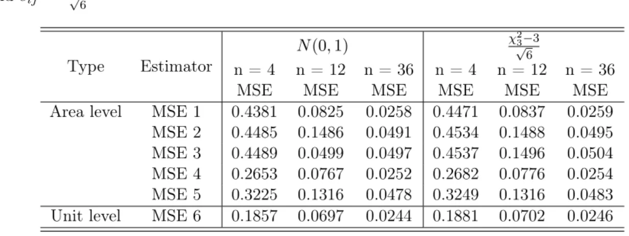
Scenario VI: We compares the random conponent with standard normal distribution and Chi-square distribution for difference sample size in each areas. We generatem= 60 areas with

Ni = 40 for 20 areas,Ni = 120 for 20 areas, and Ni = 360 for the last 20 areas. A stratified

3.5 Conclusion 26 and eij ∼ χ 2 5−3 √ 6 Type Estimator N(0,1) χ_√23−3 6 n = 4 n = 12 n = 36 n = 4 n = 12 n = 36

MSE MSE MSE MSE MSE MSE

Area level MSE 1 0.4381 0.0825 0.0258 0.4471 0.0837 0.0259 MSE 2 0.4485 0.1486 0.0491 0.4534 0.1488 0.0495 MSE 3 0.4489 0.0499 0.0497 0.4537 0.1496 0.0504 MSE 4 0.2653 0.0767 0.0252 0.2682 0.0776 0.0254 MSE 5 0.3225 0.1316 0.0478 0.3249 0.1316 0.0483 Unit level MSE 6 0.1857 0.0697 0.0244 0.1881 0.0702 0.0246

Table 3.6: Comparison of Area level and Unit level Estimator - eij ∼N(0,1),eij ∼ χ

2 3−3

√ 6

Table 3.6 shows the comparison between unit-level and area-level model for difference random component distribution with difference sample sizes. The standard error for using random component with normal distribution has slightly smaller than using Chi-square distribution. For the sample size is 4, the difference between area-level EBLUP with regression estimator (MSE 4) for standard normal and chi-square distribution is 0.0009. For the sample size is 36, the difference shrinks to 0.0002. For the EBLUP estimator in unit-level (MSE 6), the difference between using standard normal distribution with chi-square distribution, are 0.0024, 0.0005, and 0.0002, respectively for n= 4, n= 12, andn= 36. It can be seen that using random component with Chi-square distribution has the same features with using standard normal distribution for the random component.

3.5

Conclusion

In this research, we conduct a simulation study to compare the five estimators in the area-level model and the EBLUP estimator for the unit-level model. We compared the MSE of the area-level and unit-level estimators for different random component distributions, different number of areas and different sample size in each area. Based on the result of the simulation study, the EBLUP for the unit-level model performs the best in all the cases. The EBLUP constructed with estimator regression one (3.5) performs the best in all five estimators in area-levels. As the sample size increases in each area, the difference between the MSE of area-level EBLUP estimator constructed with the regression estimator and the MSE of the EBLUP unit-level estimator approaches zero. That just matches the concluded in the property of the small area estimators. Therefore, we suggest constructing an EBLUP estimator with regression estimator in the area-level model. For the unit-level model, we suggest constructing EBLUP estimator.

References

References

Battese, G. E., Harter, R. M., and Fuller, W. A. (1988). An error-components model for prediction of county crop areas using survey and satellite data. Journal of the American Statistical Association, 83(401):28–36.

Binder, D. A. (1983). On the variances of asymptotically normal estimators from complex surveys. International Statistical Institute, pages 279–292.

Fay, R. E. I. and Herriot, R. A. (1979). Estimates of income for small places: An application of james-stein procedures to census data. Journal of the American Statistical Association, 74(366a):269–277.

Hidiroglou, A. M. and You, Y. (2016). Comparison of unit level and area level small area estimators. Survey Methodology.

Johnson, A. L. (2016). Agricultural labor in midwestern united states specialty cropping systems. Graduate Theses and Dissertations.

Kim, J. K. and Skinner, C. (2013). Weighting in survey analysis under informative sampling. Biometrika, 100:385–398.

Lumley, T. and Scott, A. (2015). Aic and bic for modeling with complex survey data. Journal of Survey Statistics and Methodology, 3:1–18.

Namazi-Rad, M. and Steel, D. (2015). What level of statistical model should we use in small area estimation? Australian New Zealand Journal Of Statistics, 57(2):275–298.

Acknowledgements

I would like to express my sincere gratitude to my major professor, Dr. Emily Berg for all the help she gave me, for her patience and time. I also would like to say thank you to the committee members, Dr. Cindy Yu, and Dr. Dan Nordman.

Appendix

A

Informative Sampling

The survey weights have played a nontrivial role in the analysis of the NAWS data. One reason for this is that the preliminary analysis of the augmented model indicates that the weights are correlated with the error in a model that simply omits the weights. We have said that a correlation between the inclusion probability and the error term can lead to biased estimators and that this is an indication that the sample design is “informative.”

The term “informative sampling” is nuanced and can lack clarity without a precise mathematical definition. The use of the term informative as an adjective for a sample design, independent of a specified model, is incomplete. The term informative describes a characteristic of a pair given by both a sample design and a model. If a design is informativefor a specified model, then estimators that neglect the design entirely (“unweighted estimators”) can be biased for a subset of the population parameters defining the model. Such “unweighted estimators” are not necessarily biased for all population parameters. As we will see through the examples below, a subset of the unweighted estimators may be unbiased, even under informative sampling. In this sense, even the statement that a sample design is informative for a model may be regarded as incomplete. To be precise, one may prefer to consider the notion of informative sampling as a descriptor of a triplet defined by design, model, and parameter.

This document aims to clarify the meaning of the elusive term “informative sampling.” First, we provide two simulated examples that overtly demonstrate how the model for the sample may differ from the model for the population. These examples are intentionally unrealistic. They intend to make obvious the nature of a bias in unweighted estimators that can result from a correlation between the inclusion probability and the model errors. The second part of the document discusses the role of informative sampling in a more practical sense. We explain how a situation in which a design is informative for a model may occur in practice. We relate these ideas to the NAWS survey example.

Simulated Example 1

Let theN = 10,000elements in the population be realizations from a model

yi =xi+ei, (A.1) where fori= 1, . . . .N, x1, . . . , xN iid ∼ U nif(1,10),e1, . . . , eN iid ∼N(0,1), andxi is independent of

ej for alli, j. The objective is to estimate the slope and intercept of this population model. In

this population model, the slope is 0, and the intercept is 1. A Poisson sample is selected with the inclusion probability for elementidefined by

πi= nπ˜i PN i=1π˜i , where ˜ πi=      10 if yi−xi=ei >0 1 if yi−xi=ei ≤0,

and we take the expected sample size to be n= 500.

Figure A.1 shows a plot of a simulated population in black with red dots for sampled elements. It is clear from the plot that the distribution of sampled elements is different from the distribution of the elements in the population. In particular, the intercept in the least squares line for sampled elements is shifted up from zero. (Recall that zero is the intercept in the population regression line.)

To further clarify the difference between the model for this population and sample, we compare the least squares regression line for the sample to the 45 degree line through the origin. The red line in Figure A.1 is the least squares regression line for the sampled elements, while the black line is the 45 degree line through the origin. The two lines have nearly the same slope, but the intercept for the regression line fit to the sampled data exceeds the intercept for the population.

Figure A.1: Illustration of the difference between the distribution of the sample and the

population for simulated example 1. Black dots: full population. Red dots: sampled elements. Black line: population regression line. Red line: least squares regression line based on the sample. For this scenario, the expected difference between the least squares estimate of the intercept based on the sample and the corresponding population parameter is

Bias( ˆβ0,OLS) =E " PN i=1yiπi PN i=1πi # .

For this simulated example, the least squares estimate of the intercept based on the sample is ˆ β0,OLS= 0.63,and PN i=1yiπi PN i=1πi = 0.65.

The bias of the least squares estimator of the intercept is 0.65 for this example.

Although the least squares estimator is biased for the intercept, the least squares estimator of the population slope (in this case, 1) is unbiased. For this sample, the least squares estimator of the slope is_βˆ_{1,OLS = 1.01. This illustrates a situation in which the sample design may be informative} for some but not all of the model parameters. Although the sample design is informative for the intercept, the design may be considered noninformativefor the slope.

Simulated Example 2

Let theN = 10,000elements in the population be realizations from a model

yi =xi+ei, (A.2) where for i= 1, . . . .N, x1, . . . , xN iid ∼N(0,1),e1, . . . , eN iid ∼ N(0,2), andxi is independent of ej

for all i, j. The objective is to estimate the slope and intercept of this population model. In this

population model, the slope is 0, and the intercept is 1. A Poisson sample is selected with the inclusion probability for elementidefined by

πi= nπ˜i PN i=1π˜i , where ˜ πi =exp(−xiyi/2 +x2i/4), (A.3)

and the expected sample size isn= 500.

Figure A.2 shows a plot of a simulated population in black with red dots for sampled elements. The red line is the least squares regression line obtained from the sampled elements. The slope of the least squares regression line is clearly strongly attenuated toward zero. The least squares estimate of the slope for this simulated example is_βˆ_{1,OLS = 0.034.}

Figure A.2: Illustration of the difference between the distribution of the sample and the

population for simulated example 2. Black dots: full population. Red dots: sampled elements. Black line: population regression line. Red line: least squares regression line based on the sample.

This scenario was constructed such that the expected value of the OLS estimator of the slope would be identically zero. Let Ii denote the sample inclusion indicator, and define the density of

the sample distribution as in Pfeffermann and Sverchkov (1999) by

fs(yi|xi) =fp(yi|xi, Ii = 1),

where fp is denotes “density” of the the joint distribution of(yi, xi, Ii) defined by the population

model (A.2) and the inclusion probability given by (A.3). Under (A.2) and (A.3), the sample densityfs(yi |xi) satisfies fs(yi |xi)∝π˜ifp(yi|xi), where fp(yi|xi) = 1 2√πexp −1 4(yi−xi) 2 .

The sample density is then

fs(yi|xi)∝exp −1 4y 2 i ,

and the distribution of the elements in the sample is a normal distribution with mean 0 and variance 2. The interaction betweenxi andei in the definition of the inclusion probability causes

the design to be informative for the slope.

An unweighted analysis of the sample data would indicate that yi andxi are unrelated. The

slope of the population regression line relating yi and xi for this scenario is 1. The inclusion

probabilities contain additional information about the relationship between yi and xi in the

population. Appropriately incorporating the inclusion probabilities in a model and/or estimation procedure can yield valid statistical inferences for population parameters.

Informative Sampling in Practice

The simulated examples above are obviously artificial. In practice, the inclusion probability would not be a direct function of yi, xi, or ei. Why might a sample design be informative for

a specified model in practice? In this section, we address this question. First, we discuss the issue using general language. We then consider how the NAWS survey relates to this general conceptualization. As an aside, we relate the ideas on informative sampling discussed in this document to the case of a retrospective study paired with a logistic regression model, a well-documented situation in which the selection mechanism is informative for a subset of the model parameters.

To understand why a design might be informative for a specified model in practice, we introduce a more general notation. Suppose an analyst would like to study the association between a response variableyi and a specified vector of covariatesxi. Let zi denote the vector of

variables that determine the sample design process. Thezimay include stratum indicators, cluster

indicators, or size measures used in probability proportional to size sampling. Letfp(yi, xi, zi)

denote the joint density of yi, xi, and zi in the population. The objective is to estimate the

conditional distribution ofyi givenxi defined formally as

fp(yi |xi) = R fp(yi, xi, zi)dzi R R fp(yi, xi, zi)dyidzi .

Define the conditional density ofyi givenxi in the sample as

fs(yi|xi) =fp(yi|xi, Ii = 1),