Self-paced learning for long-term tracking
James Steven Supanˇciˇc III
Deva Ramanan
Dept. of Computer Science @ University of California, Irvine
[email protected] [email protected]Abstract
We address the problem of long-term object tracking, where the object may become occluded or leave-the-view. In this setting, we show that an accurate appearance model is considerably more effective than a strong motion model. We develop simple but effective algorithms that alternate between tracking and learning a good appearance model given a track. We show that it is crucial to learn from the “right” frames, and use the formalism of self-paced cur-riculum learning to automatically select such frames. We leverage techniques from object detection for learning ac-curate appearance-based templates, demonstrating the im-portance of using a large negative training set (typically not used for tracking). We describe both an offline algo-rithm (that processes frames in batch) and a linear-time on-line (i.e. causal) algorithm that approaches real-time per-formance. Our models significantly outperform prior art, reducing the average error on benchmark videos by a fac-tor of 4.
1. Introduction
Object tracking is a fundamental task in video process-ing. Following much past work, we consider the scenario where one must track an unknown object, given a known bounding box in a single frame. We focus on long-term tracking, where the object may become occluded, signifi-cantly change scale, and leave/re-enter the field-of-view.
Our approach builds on two key observations made by past work. The first is the importance oflearningan ap-pearance model. We learn adaptive discriminative models that implicitly encode the difference in appearance between the object and the background. Such methods allow for the construction of highly-tuned templates that are resistant to background clutter. However, a well-known danger of adaptively learning a template over time is the tendency to drift [1]. Our main contribution is an algorithm that mini-mizes drift by carefully choosing which frames from which to learn, using the framework of self-paced learning [2,3].
The second observation is the importance ofdetection,
Figure 1. Our tracker uses self-paced learning to select reliable frames from which to extract additional training data as it pro-gresses (shown inred). We use such frames to define both positive examples and a very-large set of negative examples (all windows that do not overlap each positive). By re-learning a model with this additional data, and re-tracking with that model, one can cor-rect the errors shown above. We show that it is crucial to revisit old frames when adding training data; in terms of self-paced learn-ing, a concept (frame) that initially looks hard may become easy in hindsight.
where an object template is globally scanned across the en-tire frame. This allows one to re-initialize lost tracks, but requires detectors resistant to background clutter at all spa-tial regions, including those far away from the object. Most prior approaches learn a detector using a small set of neg-atives. We show that using a large set of negatives signif-icantly improves performance, but also increases computa-tion. We address the latter issue through the use of solvers that can be warm-started from previous solutions [4].
Self-paced learning: Curriculum learning is an ap-proach inspired by the teaching of students, where easy con-cepts (say, a model learned from un-occluded frames) are taught before complex ones (a model learned from frames with partial occlusions) [2]. In self-paced learning, the student learner must determine what is easy versus com-plex [3]. One natural application of such a strategy would
label frames as easy or complex as they are encountered by an online tracker. One could then update appearance mod-els after the easy frames. We show that it is crucial to revisit old frames when learning. In terms of self-paced learning, a student might initially think a concept is hard; however, once that student learns other concepts, it may become easy in retrospect.
Transductive learning:A unique aspect of our learning problem is that it is transductive rather than inductive [5]: when tracking a face, the learned model need not generalize to all faces, but only separate the particular face and back-ground in the video. In some sense, we want to “over-fit” to the video. Following [5], we use a transductive strategy for selecting frames; rather than choosing a frame that scores well under the current model (as most prior work does), we choose a frame that when selected for learning, produces a model that well-separates the object from the background. We demonstrate that the latter scheme performs better be-cause it is naturally retrospective.
Evaluation: We evaluate our method on a large-scale benchmark suite of videos. Part of our contribution is a baseline detector that tracks by detection without any on-line learning or temporal reasoning; the detector is learned from the first labeled frame. Surprisingly, we demonstrate that a simple linear template defined on HOG features out-performsstate-of-the-art trackers, including the well-known Predator TLD-Tracker [6] and MIL-Tracker [7]. We believe this disparity exists because detection is an undervalued as-pect of tracking; invariant gradient descriptors and large-scale negative training sets appear crucial for building good object detectors [8], but are insufficiently used in tracking. We use this baseline as a starting point, and show that one can reduce error by afactor of 4with our proposed self-paced transduction framework.
Computation:Our detection-based approach learns ap-pearance models from large training sets with hundreds of thousands of negative examples. Our self-paced learning scheme requires learning putative appearance models for each candidate image. To address these computational bur-dens, we make use of dual coordinate descent SVM solvers that can be “warm-started” from previous solutions. Our solvers are efficient enough to the point where detection (implemented as a convolution) is the computational bottle-neck, which can further be ameliorated with parallel com-putations. This means that our tracker is near real-time as present, and could readily be real-time with hardware im-plementations.
1.1. Related work
We refer the reader to the survey from [9] for a broad description of related work. Many object trackers can be differentiated between their choice of appearance models and inference algorithms.
Appearance models: Because object appearance is likely to change over time, many tracks update appearance models through color histogram tracking [10] and online adaption [11]. Generative subspace models of appearance are common [12,13], including recent work that makes use of sparse reconstructions [14,15]. Other methods have fo-cused on discrimative appearance models [16], often trained with boosting [17,18] or SVMs [19,20]. Our work is simi-lar to these latter approaches, though we focus on the prob-lem of carefully choosing a subset of frames from which to learn a classifier.
Inference algorithms:To capture multiple hypotheses, many trackers use sampling-based schemes such as particle filtering [21,22] or Markov-chain Monte-Carlo techniques [23,24]. Such methods may require a large number of par-ticles to track objects in clutter. We show that a discrete first-order dynamic model (which is straightforward to op-timize with dynamic programming) can accurately reason about multiple hypotheses. Moreover, our experiments sug-gest that multiple hypotheses may not even be necessary given a good appearance model; in such cases, tracking by detection is a simple and effective inference strategy.
Semi-supervised tracking: Semi-supervised and trans-ductive approaches have been previously used in track-ing. Semi-supervised [6, 7,25] trackers tend to proceed in a greedy online fashion, not revisiting past decisions. We show retrospective learning is important for correct-ing errors in the past. Transductive approaches [26, 27] are limited by the fact that the general transductive prob-lem is highly non-convex and hard to solve. We show that transduction can be effectively applied for the isolated sub-problem of frame selection (for self-paced learning).
2. Approach
Our tracker operates by iterating over three stages. First, itlearnsa detector given a training set of positives and neg-atives. Second ittracksusing that learned detector. Third, itselectsa subset of frames from which to re-learn a detec-tor for the next iteration. After describing each stage, we describe our final algorithms in Sec.3.
2.1. Learning appearance with a SVM
Assume we are given a set of labeled frames, where we are told the location of the object. Initially, this is the first frame of a video. We would like to learn a detector to ap-ply on the remaining unlabeled frames. We writeΛ for a set of frame-bounding box{(ti, bi)}pairs. We extract posi-tive and negaposi-tive examples fromΛ, and use them to learn a
Time
Position
T S
Figure 2. We use dynamic programming to maintain multiple
track hypothesis over time. We visualize detections as boxes, the best previous transition leading to a give detection as a solid arrow, and non-optimal legal transitions with a dotted line. Note that the most-likely track at frame T (in green) can be revised to an alter-nate track hypothesis at a later frame S (in blue). We find that such reasoning provides a modest increase in performance.
linear SVM: LEARN(Λ) = argmin w λ 2w·w+ (1) X ti∈Λ h max(0,1−w·φti(bi)) + X b6=bi max(0,1 +w·φti(b)) i
where φti(bi) extracts appearance (e.g., HOG) features from bounding box bi in frame ti. For each frame ti in Λ, we extract a single positive example at bounding box
biand extract a large set of negative examples at all other non-overlapping bounding boxes. We use a fixed regular-ization parameterλfor all our experiments. We solve the above minimization using a quadratic programming (QP) solver [4]. For convenience, we defineOBJ(Λ)to be the minobjective value corresponding to theargminfrom (1).
2.2. Tracking as shortest-paths
We formulate the problem of finding the optimal track
y1:N = {y1, . . . yN}given the known location in the first famey1and modelwby solving a shortest path problem on
a trellis graph shown in Fig.2. For each frame, we have a set of nodes, or states, representing possible positions of the object in that frame. Between each pair of frames, we have a set of edges representing the cost of transitioning from a particular location to another location:
T RACK(y1, w, N) = argmin y1:N N X t=2 π(yt, yt−1)−w·φ(t, yt) (2)
Local cost: The second term defines the local cost of placing the object at locationytin frame xt as the nega-tive SVM score ofw. We experimented with calibrating the score to return a probability, but did not see a significant change in performance.
Pairwise cost: We experimented with many different definitions for the pairwise costπ. In general, we found a thresholded motion model to work well in most scenarios
0 0.1 0.2 0.3 0.4 0.5 0.6 0.7 0.8 0.9 1 0.5 0.6 0.7 0.8 0.9 1 ROC Comparison
False Positive Rate
True Positive Rate
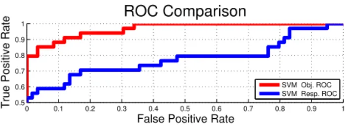
SVM Obj. ROC SVM Resp. ROC
Figure 3. Given an initial detectorw, we consider different meth-ods for selecting frames in our SELECT stage. We deem a selected frame as a true positive if the estimated track location correctly overlaps the ground-truth. Frames selected based on the SVM ob-jectivevalue in (3) greatly outperform frames selected on SVM response.
(where the pairwise cost is 0 for transitions that are consis-tent with measured optical flow and∞otherwise). Finally, to model occlusions, we augmentytwith a dummy occlu-sion state with a fixed local cost.
We compute the best track by solving the shortest-path problem using dynamic programming [28]. We also ex-perimented with an uninformative priorπ(yt, yt−1); in this
case, the best track is given by independently selecting the highest scoring location in each frame (“tracking by detec-tion”).
2.3. Selecting good frames
Our tracker operates by sequentially re-learning a model from previously-tracked frames. To avoid template drift, we find it crucial to select “good” frames from which to learn. Given a set of frames used for learningΛand an estimated tracky1:N, we estimate a new set of good frames:
SELECT(Λ, y1:N) = Λ∪(t, yt) where
t= argmin t06∈Λ
OBJ(Λ∪(t0, yt0)) (3) where we definet6∈Λto refer to frames that are not in any frame-location pair inΛ. The above select function com-putes the frame, that when added to the training setΛ, pro-duces the lowest SVM objective. We generalize the above function to return aK-element set by independently finding the (K− |Λ|) frames with the smallest increase in the SVM objective, written asSELECTK(Λ, y1:N).
Why use OBJ? Our approach directly follows from strategies for data selection in self-placed learning [3] and label assignment in transductive learning [5]. A more stan-dard approach may be to simply select the frame with the strongest model responsew·φ(t, yt); Fig.3shows that this a poorer predictor of correct frames that should be used for learning. To build intuition as to why, consider tracking a face that rotates from frontal to profile. A model learned on frontal poses may score poorly on a profile face. However, a model (retrospectively) learned from frontal and profile faces may still produce a good discriminant boundary (and hence a low SVM objective).
3. Algorithm
We now describe an online and an offline algorithm that make use of the previously-defined stages.
3.1. Online (causal) tracker
Our online algorithm is outlined in Algorithm 1. Intu-itively, at each frame: we re-estimate the best track from the first to the current frame using the current model. We then select half of the observed frames to learn/update an appearance model, which is used for the next frame. A cru-cial aspect of our algorithm is that can select frames that were previously rejected (unlike, for example [6]).
Input:y1 1 t←1; 2 Λ← {(t, yt)}; 3 w←LEARN(Λ); 4 whilet < N do 5 y1:t←T RACK(y1, w, t); 6 Λ←SELECTt/2(Λ, y1:t); 7 w←LEARN(Λ); 8 t←2t 9 end
Algorithm 1:For each frame t, our online algorithm outputs the best track found up until then. However, every power-of-two frames, it learns a new model while revisiting past frames to correct mistakes made under previous models. This allows our tracker be linear time
O(N)while still being a “retrospective” learner.
Efficiency: A naive implementation of an online al-gorithm would be very slow because it involves solving a shortest-path problem and learning an SVM at every timestep. Moreover, theSELECT function requires learn-ing (t) SVMs at each iteration (in order to evaluate OBJ for each possible frame to add). Assuming one can train linear SVMs in linear time, this would make computationO(N3).
We make two modifications to considerably reduce compu-tation. First, we only apply these expensive operations on batches of frames that double in size (Line 8). Secondly, we re-use solutions of previously-solved SVMs to warm-start new SVM problems. We do this by initializing the dual coordinate descent solvers of [4] with previously-computed dual variables. In practice, we find that evaluating OBJ for each possible frame is constant time because only a single convolution is required (discussed further in Sec.4). This means that the SELECT function scales linearly witht, making each iteration of the main loopO(t). Because our batch procedure requires onlylog2N iterations, total com-putation isN +N/2 +N/4 +. . . = O(N) . We also observe a linear scaling of computation in practice.
Initial frame
Iteration 1
Iteration 2
Iteration 3
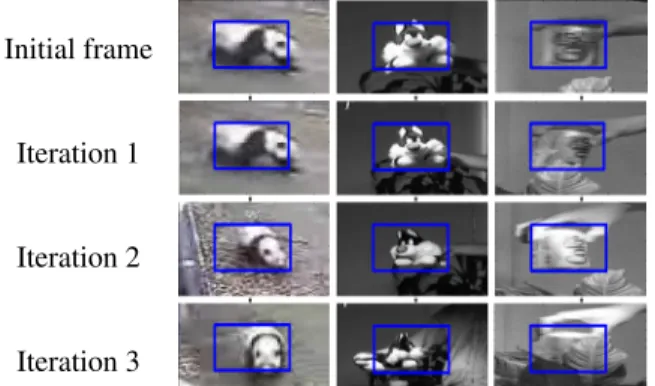
Figure 4. On the top, we show the initial labeled frame for 3 videos. In the next3 rows, we show specific examples that are added over 3 iterations of offline learning. Our model slowly ex-pands to capture more difficult appearances (or “concepts” in cur-riculum learning).
3.2. Offline tracker
Alg.2describes our off-line algorithm. It operates sim-ilarly to our online algorithm, but it has access to the en-tire set of frames in a video. We iterate between tracking (over the whole video) and learning (from a select subset of frames) for a fixed number of iterationsK. As in curricu-lum learning, we found it useful to learn from the easy cases first. We exponentially grow the number of selected frames such that at the last iteration, 50% of all frames are selected. We found that little is gained by iterating more thanK= 4 times (shown qualitatively in Fig. 4 and quantitatively in Fig.6). Input:y1 1 Λ← {(1, y1)}; 2 w←LEARN(Λ); 3 fori= 1 :Kdo 4 y1:N ←T RACK(y1, w, N); 5 Λ←SELECTr(Λ, y1:N) where r= N2 i K; 6 w←LEARN(Λ); 7 end
Algorithm 2: Our offline algorithm performs a fixed number (K) of iterations. During each iteration, it up-dates the track, selects ther “easiest” new frames of training examples, and re-trains using these examples.
4. Implementation
We now discuss various implementation details for ap-plying our algorithms.
Tracking: We implement theT RACK subroutine by using dynamic programming, which requiresO(s2N)time
whereN is the number of frames andsis the number of states per-frame. To reduce computational costs we limits
to be the top 25 new detections. Thus, assuming all videos are of some fixed resolution, the complexity of our tracking
algorithm is O(N) given a fixed model.
Repeatedly-learning SVMs: Each call toLEARN re-quires training a single SVM, and each call toSELECT
requires training (t)SVMs, needed to evaluate the SVM objective OBJ for each possible frame to select. Training each SVM from scratch would be prohibitively slow due to our massive negative training sets. We now show how to use the dual coordinate descent method of [4] to “warm-start” SVM training using previous solutions.
Dual QP:We write the dual of (1) by writing a training example asxiand its labelyi∈ {−1,1}:
max 0≤α≤C− 1 2 X i,j αiyixi·xjyjαj+ X i αi (4)
KKT conditions allow us to reconstruct the primal weight vector asw = P
αiyixi. We represent our models both with a weight vectorw, and implicitly through a cached col-lection of non-zero dual variables{αi}and support vectors
{xi}. We include all positive examples in our cache (even if they are not a support vector) because they require essen-tially no storage, and may become support vectors during subsequent optimizations as described below.
Warm-start:Given a modelwand its dual variablesαi and support vectorsxi, we can quickly learn a new model and estimate the increase in OBJ due to adding an additional framet. We perform one pass of coordinate descent on ex-amples from this new frame as follows: we run the model
won frametand cache examples with a non-zero gradient in the dual objective (4). One can show this is equivalent to finding margin violations; e.g. negative examples that score greater than−1and positive examples that score less than 1[4]. This can be done with a single convolution that eval-uates the current modelwon framet. In practice, we find that our dual QP converges after a small fixed number of co-ordinate descent passes over the cache, making the overall training time dominated by the single convolution.
5. Results
Benchmark evaluation:We define a test suite of videos and ground truth labelings by merging the test videos of [7,6]. We show a sampling of frames in Fig.5. Previous approaches evaluate mean displacement in pixels or thresh-olded detection accuracy. In our experience, displacement error can be ambiguous because it is not scale-invariant and can be somewhat arbitrary once an algorithm looses track. Furthermore, pixel displacement is undefined for frames where the object is occluded or leaves the camera view (common in long-scale tracking). Instead, we use follow [6] and define an estimated object location as correct if it suf-ficiently overlaps the ground-truth. We then compute true positive and missed detections, producing a finalF1score.
To further spur innovation, we have released our combined
benchmark dataset, along with all our source code (avail-able through the author’s website).
Overall performance: We evaluate our performance against state-of-the-art trackers with published source (TLD and MIL Track) code in Fig. 7 and Table 1. TLD re-quires a minimum window size for the learned model; the default value (of 24×24pixels) was too large for many of the benchmark videos. We manually tuned this to 16 pixels, but this reduced performance on other videos (be-cause this increases the number of possible candidate lo-cations). We show results for both parameter settings, in-cluding results for tuning this parameter on aper-video ba-sis. On two videos, MILTrack loses track by frame 500 and so we only report accuracy over those initial 500 frames. Even when giving past work these unfair advantages, our fi-nal system (without any per-video tuning) significantly out-performs past work 93% vs76%. Our online algorithm slightly underperforms our offline variant, with an average
F1 of 91%. For completeness, we also include results for
mean displacement error (for the subset of videos with no occlusion or field-of-view exits) in Table3. In terms of dis-placement error, our method compares favorably to much recent work, but does not quite match the recent perfor-mance of [24]. We hypothesize this gap exists because we resolve object location up to a HOG cell and not an individ-ual pixel. We posit that overlapping cells or post-processing temporal smoothing would likely reduce our displacement error.
Speed: Our final algorithm runs at about201threal-time. In the next diagnostic section, we describe variants, many of which are real-time while still outperforming prior art. The current bottleneck of our algorithm is the repeated evalua-tion of detectors on image frames. Because this convoluevalua-tion operation is straightforward to parallelize, we believe our full system could also operate at real-time given additional optimizations.
5.1. Diagnostics
In Table2, we analyze various aspects of our system that are important for good results. We point out those obser-vations that seem inconsistent with the accepted wisdom in the tracking literature. We refer to specific rows in the table using its label in the first column (e.g., “D1”).
Detection: We begin with a “naive” tracking-by-detection baseline. Our baselineLEARNs a detector from the initial labeled frame, and simply returns the highest scoring location at each subsequent frame. Surprisingly, even without additional learning or tracking, our baseline (D1) produces aF1score of 73%, outperforming MILTrack
and comparable to TLD. Most prior work on learning for detection uses a small set of negatives, usually extracted from windows near the object. We compare to such an ap-proach (D2), and show that using a large set of negatives
Partial Occlusion Illumination Changes Object Deformation Out of Plane Rotation
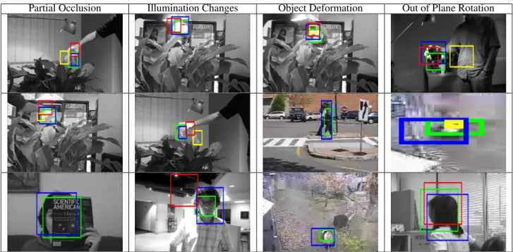
Figure 5. Our test videos present numerous challenges, including (from left to right): partial occlusion, illumination changes, object deformation, and out of plane rotation. Ground Truth is Green . TLD is Yellow ; MIL Track is Red ; Our Tracker is Blue. If there is no rectangle for a tracker, then that tracker signaled occlusion for the frame. In general, our system is able to track correctly through such challenging scenarios. Our large negative training sets and retrospective learning greatly reduce the probability of false positives.
n = 1 n = N/64 n = N/32 n = N/16 n = N/8 n = N/4 n = N/2 0.2 0.3 0.4 0.5 0.6 0.7 0.8 0.9 1 Iteration Performance (f1)
Performance by Training Iteration
coke11 david faceocc faceocc2 girl motocross sylv tiger1 tiger2 volkswagen panda pedestrian1
Figure 6. Offline learning in action. As we increase the number of latently labeled training frames (from 1 to 50%), performance generally increases. For many videos, the initial model learned on the first frame is already quite accurate. We discuss this somewhat surprising observation at length in the text.
is crucial for good performance. We see this observation as emphasizing an under-appreciated connection between tracking and detection; it is well-known in the object de-tection community that large training sets of negatives are crucial for good performance [8].
Motion: Adding a motion model to our baseline detec-tor improves performance from 73% (D1) to 76% (D5,D6). However, a standard first-order motion model (that favors stationary objects) is not particularly effective, improving performance to only 74% (D4). Our optical-flow-based
mo-tion model works much better. A single-hypothesis greedy tracker – that greedily enforces the dynamic model in (2) given the best location in the previous frame – improves performance to 76% (D3). This suggests that multiple hy-pothesis tracking may not be crucial for good performance. Furthermore, the improvement due to motion in our final system with learning is even lower; without any motion model, we still perform at 89% (D8). We find thatthe bet-ter the detector, the less advantage can be gained from a motion model.
Learning:Learning is the most crucial aspect of our sys-tem, improving performance from 76% (D5) to 91% (C6) for our online algorithm (and even more for our off-line). We construct a restricted version of our online algorithm that does not require revisiting previous frames. We do this by not allowing SELECT to accept a previously-rejected frame, and not allowing TRACK to edit a previously-estimated location. This restriction virtually eliminates all benefits of learning, producing aF1of 77% (D7). This
sug-gests that its vital to edit previous tracks to produce bet-ter examples for retrospectivelearning. Secondly, naively
SELECTing all previously-seen frames for learning also significantly decreases performance to 84% (D9). This sug-gests that selecting a good subset of reliable frames is also important. Finally, our OBJ-based criteria for frame selec-tion outperforms the tradiselec-tional SVM response, 91% (C6) vs 89% (D10). The performance increase is largest (up to 10%) for difficult videos such as Panda and Motocross.
Benchmark video comparison (F1score)
# Coke David Face1 Face2 Girl Moto-x Sylvester Tiger1 Tiger2 VW Panda Pedestrian Mean
C1 LK-FB [29] 40.00 100.0 99.43 99.43 100.0 00.04 72.38 28.16 27.39 04.00 05.13 10.71 42.09
C2 MIL Track[7] 55.00 95.00 99.44 100.0 93.00 01.00† 97.00 82.00 85.00 58.00†36.27 63.76 72.12†
C3 TLD (min=24) [6] ERR 96.77 41.96 99.43 88.29 ERR 94.40 62.85 48.64 ERR ERR ERR ERR
C4 TLD (min=16) 90.26 95.45 100.0 60.81 85.08 48.58 92.50 44.06 50.48 95.24 69.68 11.04 70.26
C5 TLD (min=better) 90.26 96.77 100.0 99.43 88.29 48.58 94.40 62.85 50.48 95.24 69.68 11.04 75.59
C6 Us [On-line] 98.21 90.32 99.71 93.25 98.02 79.08 91.01 91.01 95.83 95.46 62.09 95.71 90.81
C7 Us [Off-line] 97.39 94.62 99.71 98.16 100.0 82.95 93.65 98.59 98.63 96.48 63.05 95.00 93.18
Table 1. Comparison of methods (F1, higher is better). ERR indicates a tracker did not run given the size of the initial object bounding box. †indicates a tracker was evaluated only on the initial (500) frames before it lost track. Our trackers place special emphasis on long term tracking and can thus recover from such failures. Both online and offline versions of our algorithm significantly outperform prior work, including various versions of TLD tuned with different hyper-parameters.
Diagnostic analysis (without learning)
# Version Coke David Face1 Face2 Girl Moto-x Sylvester Tiger1 Tiger2 VW Panda PedestrianMean
D1 Tracking by Detection 88.69 33.33 99.71 96.31 95.05 25.41 88.80 90.14 83.56 67.43 31.97 75.71 73.01
D2 TBD with sub-sampling 73.04 17.20 37.08 38.65 35.64 33.80 81.72 50.70 47.95 70.99 7.89 12.86 42.29
D3 Single track hypothesis 78.00 24.24 99.71 96.31 96.04 37.26 90.67 92.95 86.30 82.95 28.79 95.00 75.68
D4 On-line w/o flow 85.21 36.55 96.31 99.71 96.04 26.26 89.92 92.95 80.28 83.22 30.29 69.74 73.87
D5 On-line 85.96 33.51 99.71 96.93 91.08 34.60 89.55 92.95 84.72 83.11 29.63 91.75 76.12
D6 Off-line 85.21 36.55 99.71 96.93 96.04 39.76 89.17 92.95 80.82 83.94 26.52 92.85 76.70
Diagnostic analysis (with learning)
D7 Fix TRACK & SELECT 91.43 35.03 99.72 93.25 95.05 29.76 91.15 91.18 80.00 89.71 40.79 89.61 77.22
D8 On-line w/o motion 97.39 88.17 99.72 93.87 99.01 64.04 92.16 94.37 93.15 95.66 53.06 95.71 88.86
D9 On-line w/ SelectAll 97.39 91.40 99.72 88.34 100.00 73.35 80.46 97.87 73.38 70.18 43.74 90.97 83.90
D10 On-line w/ RespSelect 98.21 89.24 99.71 95.70 94.05 72.06 88.67 98.57 93.70 92.07 52.64 93.57 89.02
Table 2. Diagnostic analysis of our system (F1, higher is better), with and without learning. Please see Sec.5.1for a detailed discussion.
Mean Center Displacement Error (MCDE)
Tracker Us[C6] Us[C7] ART[24] LRSVT[25] TLD MIL[7] Frag[30] PROST[31] NN[32] OAB1[33]
Code Yes Yes No No Yes Yes Yes No Yes Yes
Sylv. 12 12 6 9 14 11 11 - - 25 Girl 17 29 11 - 21 32 27 19 18 48 David 10 7 3 7 7 23 46 15 16 49 Face1 10 11 8 12 18 27 6 7 7 44 Face2 14 13 6 10 17 20 45 17 17 21 Tiger1 4 4 5 8 15 15 40 - - 35 Tiger2 7 5 5 13 30 17 38 - - 34 Coke 7 7 - 12 9 21 63 - - 25 Mean 10 11 6* 10* 16 21 35 15* 15* 35
Table 3. Mean Center Displacement Error (MCDE), where lower is better. * indicates a given tracker did not report results on all videos. Though we believe theF1 score (see Table1) is a more accurate measure, we report MCDE for completeness. Our trackers generally compare favorably to other state of the art algorithms. We conjecture that our pixel displacement error would decrease if we resolved object locations up to pixels and not just HOG cells. See Sec.5for more discussion.
5.2. Conclusion
We have a described a simple but effective system for tracking based on the selection of trustworthy frames for learning appearance. We have performed an extensive di-agnostic analysis across a large set of benchmark videos that reveals a number of surprising results. We find the task of learning good appearance models to be crucial, as com-pared to say, maintaining multiple hypothesis for tracking. To learn good appearance models, we find it important to use large sets of negative training examples, and to retro-spectivelyedit and select previous frames for learning. To
do so in a principled and efficient manner, we use the for-malism of self-paced learning and online solvers for SVMs. Our tracker handles long videos with periods of occlu-sion/absence and large scale changes. Our benchmark anal-ysis suggests we do so with significantly better accuracy than prior art. Our algorithms are linear time and so asymp-totically efficient. We believe that a parallelized implemen-tation could easily lead to real-time performance with sig-nificant real world applications.
Acknowledgements:Funding for this research was pro-vided by NSF Grant 0954083, ONR-MURI Grant
N00014-Cumulati v e F1 Pedestrain 1 Panda Volkswagen Tiger2 Tiger1 Sylvester Motocross Girl Face Occ 2 Face Occ 1 David Coke Can
Our's Offline Our's Online TLD MIL Track
Figure 7. We compareF1 scores, accumulated across 12 bench-mark test videos. The maximum accumulated score is 12. Our trackers significantly reduce error, compared to prior work. Most of the improvement comes from a few “challenging” videos containing significant occlusions and scale challenges, including Pedestrian, Panda, and Motorcross. See Table1for additional nu-meric analysis.
1010933, and the Intel Science and Technology Center -Visual Computing.
References
[1] L. Matthews, T. Ishikawa, and S. Baker, “The template up-date problem,”IEEE PAMI, 2004.1
[2] Y. Bengio, J. Louradour, R. Collobert, and J. Weston, “Cur-riculum learning,” inICML, pp. 41–48, ACM, 2009.1 [3] M. Kumar, B. Packer, and D. Koller, “Self-paced learning for
latent variable models,”NIPS, 2010.1,3
[4] R. Fan, K. Chang, C. Hsieh, X. Wang, and C. Lin, “Liblin-ear: A library for large linear classification,”JMLR, vol. 9, pp. 1871–1874, 2008.1,3,4,5
[5] V. Vapnik,The nature of statistical learning theory. springer, 1999.2,3
[6] Z. Kalal, K. Mikolajczyk, and J. Matas, “Tracking-Learning-Detection,”IEEE PAMI, 2011.2,4,5,7
[7] B. Babenko, M. Yang, and S. Belongie, “Robust object track-ing with online multiple instance learntrack-ing,” IEEE PAMI, vol. 33, no. 8, pp. 1619–1632, 2011.2,5,7
[8] N. Dalal and B. Triggs, “Histograms of oriented gradients for human detection,” inCVPR, IEEE, 2005.2,6
[9] A. Yilmaz, O. Javed, and M. Shah, “Object tracking: A sur-vey,”Acm Computing Surveys (CSUR), vol. 38, no. 4, p. 13, 2006.2
[10] D. Comaniciu, V. Ramesh, and P. Meer, “Kernel-based ob-ject tracking,”IEEE PAMI, vol. 25, no. 5, 2003.2
[11] A. Jepson, D. Fleet, and T. El-Maraghi, “Robust online ap-pearance models for visual tracking,”IEEE PAMI, vol. 25, no. 10, pp. 1296–1311, 2003.2
[12] D. Ross, J. Lim, R. Lin, and M. Yang, “Incremental learning for robust visual tracking,”IJCV, vol. 77, no. 1, 2008.2 [13] K. Lee, J. Ho, M. Yang, and D. Kriegman, “Visual tracking
and recognition using probabilistic appearance manifolds,”
CVIU, vol. 99, no. 3, pp. 303–331, 2005. 2
[14] X. Mei and H. Ling, “Robust visual tracking and vehicle classification via sparse representation,”IEEE PAMI, vol. 33, no. 11, pp. 2259–2272, 2011.2
[15] B. Liu, J. Huang, L. Yang, and C. Kulikowsk, “Robust track-ing ustrack-ing local sparse appearance model and k-selection,” in
CVPR, IEEE, 2011.2
[16] R. Collins, Y. Liu, and M. Leordeanu, “Online selection of discriminative tracking features,” IEEE PAMI, vol. 27, no. 10, pp. 1631–1643, 2005.2
[17] H. Grabner, C. Leistner, and H. Bischof, “Semi-supervised on-line boosting for robust tracking,”ECCV, pp. 234–247, 2008.2
[18] S. Avidan, “Ensemble tracking,”IEEE PAMI, vol. 29, no. 2, pp. 261–271, 2007.2
[19] S. Avidan, “Support vector tracking,”IEEE PAMI, vol. 26, no. 8, pp. 1064–1072, 2004.2
[20] S. Hare, A. Saffari, and P. Torr, “Struck: Structured output tracking with kernels,” inICCV, 2011.2
[21] M. Isard and A. Blake, “Condensation-conditional density propagation for visual tracking,”IJCV, 1998.2
[22] K. Okuma, A. Taleghani, N. Freitas, J. Little, and D. Lowe, “A boosted particle filter: Multitarget detection and track-ing,”ECCV, pp. 28–39, 2004.2
[23] J. Kwon and K. Lee, “Visual tracking decomposition,” in
CVPR, pp. 1269–1276, IEEE, 2010.2
[24] D. Park, J. Kwon, and K. Lee, “Robust visual tracking using autoregressive hidden markov model,” inCVPR, pp. 1964– 1971, IEEE, 2012.2,5,7
[25] Y. Bai and M. Tang, “Robust tracking via weakly supervised ranking svm,” inCVPR, pp. 1854–1861, IEEE, 2012.2,7 [26] Y. Wu and T. Huang, “Color tracking by transductive
learn-ing,” inCVPR, vol. 1, pp. 133–138, IEEE, 2000.2
[27] Y. Zha, Y. Yang, and D. Bi, “Graph-based transductive learn-ing for robust visual tracklearn-ing,”Pattern Recognition, vol. 43, no. 1, pp. 187–196, 2010.2
[28] A. Buchanan and A. Fitzgibbon, “Interactive feature tracking using kd trees and dynamic programming,” inCVPR, vol. 1, pp. 626–633, IEEE, 2006.3
[29] Z. Kalal, K. Mikolajczyk, and J. Matas, “Forward-Backward Error: Automatic Detection of Tracking Failures,” ICPR, 2010.7
[30] A. Adam, E. Rivlin, and I. Shimshoni, “Robust fragments-based tracking using the integral histogram,” inCVPR, vol. 1, pp. 798–805, IEEE, 2006.7
[31] J. Santner, C. Leistner, A. Saffari, T. Pock, and H. Bischof, “Prost: Parallel robust online simple tracking,” in CVPR, pp. 723–730, IEEE, 2010.7
[32] S. Gu, Y. Zheng, and C. Tomasi, “Efficient visual object tracking with online nearest neighbor classifier,” ACCV, pp. 271–282, 2011.7
[33] H. Grabner, M. Grabner, and H. Bischof, “Real-time tracking via on-line boosting,” inProc. BMVC, vol. 1, 2006.7