NBER WORKING PAPER SERIES
ESTIMATING AND TESTING BETA PRICING MODELS:
ALTERNATIVE METHODS AND THEIR PERFORMANCE IN SIMULATIONS Jay Shanken
Guofu Zhou Working Paper 12055
http://www.nber.org/papers/w12055
NATIONAL BUREAU OF ECONOMIC RESEARCH 1050 Massachusetts Avenue
Cambridge, MA 02138 February 2006
Shanken is the Goizueta Chair in Finance at Emory University and a Research Associate at NBER and Zhou is from Washington University in St. Louis. This paper earlier version of the paper circulated under the titles “Analytical cross-sectional tests of asset pricing models” and “On cross-sectional stock returns: maximum likelihood approach.” We are grateful to Phil Dybvig, Wayne Ferson, Will Goeztmann, Campbell Harvey, John Heaton, Ravi Jagannathan, Raymond Kan, Dongcheol Kim, Robert Korajczyk, Mark Loewenstein, Cesare Robotti, William Schwert (the managing editor), seminar participants at Northwestern University, Univerisyt of Michigan, University of Missouri-Columbia, and the 2005 SBFSIF conference, and especially an anonymous referee for several insightful and detailed comments that substantially improved the paper. We also appreciate the outstanding research of Jun Tu. The views expressed herein are those of the author(s) and do not necessarily reflect the views of the National Bureau of Economic Research.
©2006 by Jay Shanken and Guofu Zhou. All rights reserved. Short sections of text, not to exceed two paragraphs, may be quoted without explicit permission provided that full credit, including © notice, is given to the source.
Estimating and Testing Beta Pricing Models: Alternative Methods and their Performance in Simulations
Jay Shanken and Guofu Zhou NBER Working Paper No. 12055 February 2006
JEL No. G12
ABSTRACT
In this paper, we conduct a simulation analysis of the Fama and MacBeth (1973) two-pass procedure, as well as maximum likelihood (ML) and generalized method of moments estimators of cross-sectional expected return models. We also provide some new analytical results on computational issues, the relations between estimators, and asymptotic distributions under model misspecification. The GLS estimator is often much more precise than the usual OLS estimator, but it displays more bias as well. A "truncated" form of ML performs quite well overall in terms of bias and precision, but produces less reliable inferences than the OLS estimator.
Jay Shanken
Goizueta Business School Emory University 1300 Clifton Road Atlanta, GA 30322 and NBER [email protected] Guofu Zhou
Olin School of Business Washington University St. Louis, MO 63130 [email protected]
1
Introduction
Explaining cross-sectional differences in asset expected returns is one of the great challenges of modern finance. Theoretical models, such as the CAPM of Sharpe (1964), Lintner (1965), and Black (1972), and the intertemporal/consumption models of Merton (1973), Breeden (1979), and Rubinstein (1976), imply that expected returns should be linear in asset betas with respect to fundamental economic aggregates. Equilibrium extensions of the Ross (1976) APT and the “mul-tivariate proxy” perspective on factor pricing models, e.g. Shanken (1987), yield similar relations. There is an enormous body of empirical research that examines these linear asset pricing relation-ships. One of the most widely used methodologies is the two-pass regression approach, known as the Fama-MacBeth procedure, developed by Fama and MacBeth (1973) and Black, Jensen and Scholes (1972). The two-pass procedure is used not only in asset pricing, but also in many other areas of finance. For example, Fama and French (1998), Grinstein and Michaely (2002) and Easley, Hvidjkaer and O’Hara (2002) apply it in analyzing corporate finance and market microstructure issues.1
The asymptotic statistical properties of the Fama-MacBeth procedure were first established in the study by Shanken (1992) and later extended by Jagannathan and Wang (1998). However, despite its widespread application, surprisingly little is known about the small-sample statistical properties of the methodology. An early simulation study by Amsler and Schmidt (1985) provides some insights, though the main focus of that paper is on multivariate tests of the linear expected return relation. A contemporaneous paper by Chen and Kan (2005) provides analytical results on estimation bias as well as some simulation evidence. Our paper attempts to fill in some of the important gaps in our knowledge, comparing the performance of the usual OLS version of the Fama-MacBeth procedure to the WLS and GLS approaches occasionally seen in the literature.2
In addition to the two-pass approach, we explore alternative analytically tractable procedures based on maximum likelihood (ML) estimation and the generalized method of moments (GMM) of Hansen (1982). The ML method is important in that it is asymptotically efficient under the classical independent and identically distributed (iid) multivariate normal returns assumption. The GMM approach is of further interest since serial correlation and conditional heteroscedasticity in the joint distribution of returns and factors is easily accommodated in making asymptotically valid
1Applications of the procedure in recent years can be found in at least 735 papers that cite Fama and MacBeth (1973), as complied by Google.
2Balduzzi and Robotti (2004) consider estimation issues related to the use of mimicking portfolios for non-traded factors.
inferences. These characteristics of the data have typically been ignored in the empirical literature, but will likely receive more attention in the future. The computational simplifications that we introduce facilitate the simulation analysis and should make these methods more accessible to researchers. We also demonstrate an equivalence between ML estimation and one form of the GMM estimator under the classical assumptions.
Application of the estimation methods considered here implicitly assumes that the expected return relation is well specified. One approach to testing this specification is to include additional cross-sectional regressors in the relation and see whether such variables are significantly related to returns. For example, Fama-MacBeth add beta-squared and residual variance in their study. This approach requires that the researcher have some idea as to the nature of the departure from the asset pricing relation and is vulnerable to the influence of data mining. In contrast, multivariate tests focus on the overall magnitude of estimated pricing deviations and have the potential to reject the null for a broad range of general alternatives. The downside, however, may be a reduction in power against particular alternatives of interest. Moreover, since the tests typically require some sort of sorting of securities into portfolios, data mining can still be a problem, e.g., Lo and MacKinlay (1990). We evaluate the actual size of various tests and power against several alternatives of interest.
One could argue that, strictly speaking, all models are false and are, at best, close approxi-mations to reality. Moreover, even if we entertain the possibility that a given asset pricing model does hold exactly, the limited power of pricing tests implies that we cannot always know whether the model is well-specified. Thus, it is inevitable that we will often, knowingly or unknowingly, estimate an expected return relation that departs from exact linearity in the betas. We derive the asymptotic distribution of the Fama-MacBeth estimator in this context, thereby providing insight into the extent to which misspecification can affect inferences about factor risk premia.
The paper is organized as follows. Section 2 reviews the statistical specification of the asset pricing model and the different versions of the Fama-MacBeth procedures. We then present the asymptotic theory for the second-pass risk premium estimators when the asset pricing restrictions are violated. In Section 3, we study the ML method and show how to obtain the parameter estimates analytically. In Section 4, we develop two analytical GMM methods that are robust to conditional heteroscedasticity and serial correlation. Extensive simulations are conducted in Section 5, to study the finite sample properties of the various approaches to estimation and testing. An empirical application is discussed in Section 6. Conclusions are offered in the final section.
2
OLS, WLS and GLS two-pass procedures
In this section, first we briefly review the standard cross-sectional model and the associated OLS, WLS and GLS two-pass estimators and tests. Then we provide asymptotic distributional results for the estimators under the alternative hypothesis that the cross-sectional pricing restrictions are not valid.
2.1 Model, estimation and tests
We assume that the asset returns are governed by a multi-factor model:
Rit=αi+βi1f1t+· · ·+βiKfKt+²it, i= 1, . . . , N, t= 1, . . . , T, (1)
where
Rit = the return on assetiin periodt (1≤i≤N),
fjt = the realization of thej-th factor in periodt (1≤j≤K), ²it = the disturbances or random errors,
and T is the number of time-series observations. Like most studies, we maintain the assumption that the disturbances are independent over time and jointly distributed each period with mean zero and a nonsingular residual covariance matrix Σ, conditional on the factors. The maximum likelihood analysis in Section 3 will also impose joint normality of the disturbances, conditional on the factors. The factors are assumed to be independent and identically distributed (iid) over time though, as demonstrated in Shanken (1992), this assumption can easily be relaxed in deriving asymptotic results for the second-pass estimators. The GMM approaches presented later in Section 4 relax the iid assumption on the disturbances as well.
The asset pricing hypothesis underlying the standard two-pass procedure is3
H0 : E[Rt] =γ01N +γ1β1+· · ·+γKβK, (2)
where E[Rt] is the N-vector of expected returns on the assets and β1, . . . , βK are N-vectors of
the multiple-regression betas. In the first stage of the two-pass procedure, estimates of the betas are obtained by applying OLS to equation (1) for each asset. Let ˆβ = ( ˆβ1, . . . ,βˆK) be the
re-sulting N ×K matrix of OLS slope estimates. For each period t, one then runs a cross-sectional
3It may be advisable to impose additional constraints if some of the factors are portfolios. See Shanken (1992). However, such constraints have usually been ignored in the two-pass literature. Our analytical results can be extended to accommodate these constraints.
regression of Rt = (R1t, . . . , RN t)0 on ˆX = [1N,β] in the second stage to get an estimator ofˆ Γ = (γ0, γ1, . . . , γK)0 = (γ 0, γa0)0, ˆ Γt= ( ˆX0X)ˆ −1Xˆ0Rt. (3) The average, ˆ ΓOLS= T X t=1 ˆ Γt/T = ( ˆX0X)ˆ −1Xˆ0R,¯ (4)
is taken as the final estimator of Γ, where ¯R is theN-vector of sample means of the asset returns.4
In the second pass, Shanken (1985), among others, proposes the use of the following GLS estimator,
ˆ
ΓGLS= ( ˆX0Σb−1X)ˆ −1Xˆ0Σb−1R,¯ (5) where Σ is the estimator of the residual covariance matrix computed as the cross product of theb fitted factor model residuals divided by T.5 Shanken (1992) proves that the GLS estimator is
asymptotically efficient.
The OLS estimator is not asymptotically efficient, in general. However, since the GLS estimator requires estimation of the inverse of the covariance matrix, it might not be expected to perform well when the sample size is small. An alternative that would seem to have potential is a weighted least-squares (WLS) estimator,
ˆ
ΓWLS= ( ˆX0Σb−1d X)ˆ −1Xˆ0Σb−1d R,¯ (6) where the weighting matrixΣbdconsists of the diagonal elements ofΣ. Litzenberger and Ramaswamyb
(1979) were perhaps the first to use this type of estimator in testing the CAPM.
The issue of whether a specific factor is priced has been of primary interest in the literature. The OLS t-ratios traditionally used for assessing the significance of factor pricing are computed as
ˆ tj = ˆ γOLS j ˆ sj/ √ T, j= 1, . . . , K, (7) where ˆγOLS
j and ˆsj are the sample mean and standard deviation of thej-th component of the time
series ˆΓt, t = 1, . . . , T. Similar ratios can be computed for the WLS and GLS estimators. The p-values are usually computed from atdistribution with degrees of freedomT−1 or from a standard normal distribution. The advantage of evaluating significance in this manner is that cross-sectional
4In some studies, betas are estimated from a rolling window of past data, further complicating the econometric analysis.
5We assumeT >(N+K) so that the usual sample covariance estimator is invertible. Shanken (1985) shows that the same estimator is obtained using the sample covariance matrix of returns.
heteroskedasticity and correlation are implicitly taken into account, as these characteristics of the distribution influence the precision of each estimator and, therefore, are reflected in the time-series variability of the estimators. However, this approach ignores estimation error in the betas.
Note that all of the two-pass estimators can be written in the following form,
ˆ
Γw = ˆAwR,¯ Aˆw = ( ˆX0WˆX)ˆ −1Xˆ0W ,ˆ (8)
where ˆW is a symmetric weighting matrix. For example, the OLS estimator is obtained with ˆW equal to the identity matrix. Under the standard iid assumption, Shanken (1992) provides the asymptotic covariance matrix for this type of estimator,
Υw= ACov(ˆΓw) = (1 +c)Ωw+ Σ∗f, (9)
where c =γa0Σ−1f γa, γa, as defined earlier, is Γ excluding the first element, Ωw = AwΣA0w, Aw is
the probability limit of ˆAw, and
Σ∗f = 0 0 0 Σf , (10)
with Σf the population covariance matrix of the K factors.6 Asymptotically standard normal
“t-ratios” are then obtained by dividing the estimates by their asymptotic standard errors. It follows that the Fama-MacBeth standard errors, computed as the times series standard errors of the estimated gammas, understate the true asymptotic standard errors by the amount cΩw.
Although this difference is fairly small in our simulations, it may be important elsewhere; see, e.g., Section 4.1 of Shanken (1992).
The usual interpretation of standard tests for factor pricing presumes that expected returns can indeed be expressed as a linear function of the betas. However, a risk premium parameter can be significantly different from zero based on the t-test, even if there are large pricing errors. Therefore, it is important to separately test the validity of the model. As mentioned earlier, a common approach to testing linearity is to include additional variables in the cross-sectional regression and evaluate the significance of these variables via the Fama-MacBeth method.
Shanken (1985) proposes a cross-sectional specification test of (2) against a general alternative,
Qc=T( ¯R−ˆγ0GLS1N −βˆγˆaGLS)0Σb−1( ¯R−γˆ0GLS1N−βˆγˆaGLS)/(1 + ˆc), (11) 6This is the limiting covariance matrix for√T times the difference between the estimator and the true parameter value.
where ˆΓGLS = (ˆγGLS
0 ,γˆaGLS0)0 and ˆc is a consistent estimator of c with the GLS weighting matrix.
Qc summarizes the estimated pricing errors across assets weighted by Σb−1, with an adjustment
in the denominator for errors in the betas. The larger the pricing errors, the larger the observed value for Qc. Intuitively, if (2) is true, Qc should not be “too far” from zero, as the errors will
be random. On the other hand, if (2) does not hold then there will be systematic deviations as well, resulting in larger values of the observed test statistic. Roll (1985) provides an interesting geometric interpretation ofQc when the factor is the return on a benchmark portfolio.7
2.2 Estimation under the alternative
Standard inference using the two-pass procedures implicitly assumes that the asset pricing restric-tion (2) is true. What happens when this restricrestric-tion is violated, as is likely to be the case in practice? The purpose of this subsection is to provide both the asymptotic distributions of the two-pass estimators under the alternative and a model specification test.
Whether the restriction is true or not, we can always project the expected return vectorE[Rt]
onto X= [1N, β],
E[Rt] =XΓw+ηw, (12)
where
Γw = (X0W X)−1X0W E[Rt] (13)
is the coefficient vector of the weighted projection andηwis the projection residual or (true) pricing
error vector. As the sample size,T, gets large, ˆΓwwill converge to Γw. This was noted previously by
Kandel and Stambaugh (1995), who study the cross-section of returns when the benchmark portfolio is inefficient. We go beyond this consistency result and derive the asymptotic distribution of the second-pass estimator when the expected return relation (2) is misspecified, extending Theorem 1 of Shanken (1992).8
Proposition 1 Given the assumptions of Section 2.1 and the additional joint normality
assump-7An identical test statistic is obtained if the sample covariance matrix of asset returns is substituted for the residual covariance matrix inQc.
8An independent paper by Kimmel (2003) considers the GLS case with the (excess) zero-beta rate constrained to equal zero. Chen, Kan and Zhang (1999) analyze the relation between statistical significance and explanatory power for expected returns allowing for model misspecification of the sort considered here. They do not address issues related to estimation error in the betas, however.
tion for the disturbances conditional on the factors, we have √ T(ˆΓw−Γw) asy ∼ N(0,Υw+ Υw1+ Υ0w1+ Υw2) (14) where Υw is given in (9), Υw1 =−(X0W X)−1 0 Σ−1f γwaη0wWΣ W X(X0W X)−1, (15)
which vanishes for the GLS estimator, and
Υw2 = (X0W X)−1 0 0 0 (η0 wWΣW ηw)Σ−1f + (η0 w⊗X0)Vw(ηw⊗X) (X0W X)−1, (16)
where Vw is the asymptotic covariance matrix of vec( ˆW −W). In the GLS case, the elements of Vw are given by
ACov( ˆwij,wˆkl) =σ∗ikσjl∗ +σil∗σjk∗ , (17)
whereσ∗
mn is the (m, n) element of Σ−1. In the WLS case, the nonzero elements are of the form,
ACov µ 1 ˆ σii , 1 ˆ σjj ¶ = 2σ 2 ij σ2 iiσjj2 , (18)
whereσmn is the (m, n) element of Σ. Vw is zero and joint normality is, therefore, not required in the OLS case.
Proof. See Appendix A.
Proposition 1 shows that the asymptotic covariance matrix of the two-pass estimator is altered when the null hypothesis is violated. There are two new terms in addition to the usual Υw. These
relate to the product of the ˆAw matrix and the pricing error vector, ηw. Υw2 is the covariance
matrix of this product while Υw1 is its covariance with the original disturbance terms that are
present in the absence of misspecification. Although Υw+ Υw1+ Υ0w1+ Υw2 is obviously positive
definite, it is not clear whether it is greater than Υw or not. Intuitively, the interaction between
the pricing errors and the errors in ˆβ introduces additional “noise” that may reduce the precision of the risk premium estimates. While we have not shown this theoretically, our simulation results support this intuition.
It is easy to verify that, when the null (2) is true and E[Rt] =XΓ, then Γw is independent of
W, i.e.,
Thus, the various two-pass estimators all converge to the same limit when the null is true. In this case, differences between the estimators are entirely attributable to random estimation errors. On the other hand, when (2) is false, the estimators may differ more systematically, as we will see in the simulation examples presented later. Thus, a test of this necessarycondition can serve as another means of evaluating expected return linearity. The asymptotic distribution of the difference of two-pass estimators follows easily from the results in Shanken (1992), yielding a simple chi-squared test as shown in the next proposition.
Proposition 2 Under the assumptions of Shanken (1992, Theorem 1), and if the (K+ 1)×N matrix, Πa= (X0Σ−1X)−1X0Σ−1−(X0X)−1X0, is of rank K+ 1, then
Jγ =T(ˆΓOLS −ΓˆGLS)0[(1 + ˆc) ˆΠaΣ ˆˆΠ0a]−1(ˆΓOLS−ΓˆGLS) asy
∼ χ2K+1, (20)
asT → ∞, where ˆΠa= ( ˆX0Σˆ−1X)ˆ −1Xˆ0Σˆ−1−( ˆX0X)ˆ −1Xˆ0.
Proof. See Appendix A.
It may be instructive to contrast the notion of model misspecification used here with that analyzed by Jagannathan and Wang (1998). They posit a “true” factor pricing model and consider the situation in which some other set of factors is employed in the estimation. Naturally, the second-pass estimator will not typically converge to the vector of coefficients in the “true” pricing model in this context and, in this sense, the estimator is biased. Consequently, thet-statistic for the risk premium associated with an observed factor can diverge to infinity (a non-zero value divided by a shrinking estimated standard error), even if the corresponding true factor is not priced. We focus, instead, on whether the observed factor is priced, i.e., whether betas on that factor are related to expected returns. Our asymptotic results allow the researcher to test hypotheses about that relation, even if the model is misspecified, in the sense that the factor betas do not fully account for the cross-sectional variation in expected returns on the given assets.9
3
The maximum likelihood approach
In this section, we provide a detailed discussion of the maximum likelihood (ML) approach as applied to the two-pass regression model. We solve the estimation problem analytically and review the associated asset pricing tests.10
9Factor portfolio constraints can easily be accommodated in this framework when some or all of the factors are portfolio spread returns.
To apply the ML approach, it is convenient to rewrite the asset pricing restrictions (2) in terms of the alphas,
H0 : α=λ01N +λ1β1+· · ·+λKβK, (21)
whereλ0 =γ0 and λk=γk−E[fk] for k= 1,2, . . . K. Then, the ML estimator of the risk premia
vector, γa, is obtained by adding the factor-mean vector to the estimator of λa= (λ1, . . . , λK)0.11
To find the ML estimator ofλa, we need to maximize the likelihood function over all the parameters
– the alphas, betas and λ= (λ0, λ0a)0. Since the parameters enter the restriction multiplicatively,
the constraints are non-linear. As a result, standard procedures are not applicable and special techniques have to be developed to solve the maximization problem.
Gibbons (1982) is the first to suggest using the ML method to estimate a special case of (21) forK = 1 with an additional constraint,λ1 =−λ0, which is an implication of the zero-beta capital
asset pricing model (CAPM). This version of the CAPM can arise if one assumes the borrowing rate differs from the lending rate. Extending a result of Kandel (1984), Shanken (1986) gives an explicit solution for the zero-beta ML estimator. Here we solve for the estimator with only (21) imposed, the case most often considered in the two-pass estimation literature. Stambaugh (1982) uses ML estimation for this specification withK = 1.
Following Shanken (1985), one can show that the ML estimator of λminimizes the function
Q(λ) = ˜a0Σb−1˜a
1 + ( ¯F+λa)0∆b−1( ¯F +λa)
, (22)
where ˜a= ˆα−λ01N−λ1βˆ1− · · · −λKβˆK and ¯F and∆ are the sample mean and covariance matrixb
of the factors. Note that the numerator is a quadratic form in the pricing errors. Minimizing this quadratic form alone yields the GLS cross-sectional regression estimator.
Given (22), the ML estimator can be computed as follows. Let
ˆ
α∗ = ˆα−(10NΣb−11N)−1(10NΣb−1α)1ˆ N, (23)
ˆ
βj∗ = ˆβj−(10NΣb−11N)−1(10NΣb−1βˆj)1N, (24) forj= 1, . . . , K and ˆβ∗= ( ˆβ∗
1, . . . ,βˆK∗). Then compute (K+ 1)×(K+ 1) matricesA and B as
A= αˆ∗0Σb−1αˆ∗ −ˆα∗0Σb−1βˆ∗ −βˆ∗0Σb−1αˆ∗ βˆ∗0Σb−1βˆ∗ , B = 1 + ¯F0∆b−1F¯ F¯0∆b−1 b ∆−1F¯ ∆b−1 . (25)
11Likewise, the factor covariance matrix is added to the asymptotic covariance matrix ofλa. This assumes that the factors are iid and that the ML estimator for the factor mean is just the sample mean, as would be the case, for example, under normality.
Now letLbe a lower-triangular matrix such thatL0L=B−1. It is straightforward to compute the
eigenvalues and eigenvectors of
|LAL0−ζI|= 0. (26)
Letting (1,˜λ0
a)0 be the eigenvector (re-scaled to make the first element be one) corresponding to the
smallest eigenvalue of (26), we have
Proposition 3 The ML estimator of λa= (λ1, . . . , λK)0 equals ˜λa and the ML estimator of λ0
is
˜
λ0= (10NΣb−11N)−110NΣb−1(ˆα−˜λ1βˆ1− · · · −˜λKβˆK). (27)
Proof. See Appendix A.
Given the ML estimate ofλ, the constrained beta estimates are obtained by running time-series regressions ofRt−˜λ01N onFt∗= (f1t+ ˜λ1, . . . , fKt+ ˜λK)0. To guard against possible coding errors,
it is advisable to verify that the first order derivatives of the likelihood function are identically equal to zero (to the accuracy of rounding error) when evaluated at the constrained estimates, i.e.,
∂Lc ∂λj =βj0Σ−1 T X t=1 [Rt−λ01N −β1(f1t+λ1)− · · · −βK(fKt+λK)] = 0, (28)
forj= 1, . . . , K. When K=1, we also have the following results for the risk premium estimator.
Proposition 4 The ML estimator of γ1, ˜γ1ML, is the root of a quadratic equation. Moreover, if
the GLS estimator satisfies ˆγ1GLS >0, we have
˜
γ1ML>γˆ1GLS (29)
and the reverse holds if ˆγGLS 1 <0.
Proof. See Appendix A.
Kandel (1984) and Roll (1985) derive a similar result when the single factor is a portfolio and the associated restriction on the risk premium estimator is imposed. Proposition 4 treats the case of a general one-factor model, without any such restriction.
The traditional analysis of linear regression estimation with an independent variable that is measured with error reveals a bias in the estimated slope coefficient toward zero. Chen and Kan (2005) show that this conclusion holds for the second-pass GLS estimator of γ1 as well. Against
this background, Proposition 4 is interesting in that it suggests that (simultaneous) ML estimation of all parameters may eliminate this errors-in-variables bias. In fact, Shanken (1992) demonstrates
that this is true, in a limiting sense, when the number of assets, N, is large. Thus, one might have conjectured that the ML estimator is, indeed, unbiased in finite samples. However, Chen and Kan (2005) have also shown that the ML estimator of γ1 does not even have a mean, shedding light
on Amsler and Schmidt’s (1985) observation that the ML estimator sometimes takes on extreme values in their simulations.
It is difficult to know what message to take away from all of this in terms of applied work. In particular, it would not make sense to focus on the moments of the ML estimator in simulations. Instead, we explore a simple “truncated” version of the ML estimator; specifically, if the absolute value of the ML estimator is more than twice that of the GLS estimator, we set the truncated estimator equal to the GLS estimator, otherwise it is unchanged.12 This estimator will have finite
moments whenever the GLS estimator does and will have the same asymptotic distribution, as T → ∞, as the GLS and ML estimators.13 Its performance in finite samples remains to be evaluated.
One approach to evaluating model specification is to use the standard likelihood ratio test of (2), which can be shown to equal Tlog(|Σ|/|e Σ|), whereb Σ is the Σ estimator evaluated at thee constrained ML estimator of the alphas and betas. This test has an asymptotic chi-squared distri-bution χ2
N−K−1. Since the chi-squared distribution is only a first-order asymptotic approximation
and tends to reject too often in this context, Jobson and Korkie (1982) suggest the use of a Bartlett (1947) correction,
LRT = [T −1
2(N +K+ 3)] log(|Σ|/|e Σ|)b
asy
∼ χ2N−K−1. (30)
Asymptotically, both tests have the same limiting distribution. The Bartlett-corrected test performs much better, however, and hence we will use this throughout. As an alternative, one can substitute the ML estimator of Γ for the GLS estimator in the earlier Qc statistic and perform an F-test of
(2). Shanken (1985) shows that the resulting statistic is actually a monotonic transformation of the likelihood ratio test for this problem.14
12Of course, other truncation rules could be considered. For example, we also examined a 5 times GLS rule with similar results.
13We make use of the fact the the mean of a random variable is finite if and only if the mean of its absolute value is finite.
14Under additional factor portfolio constraints of the multi-beta CAPM, Velu and Zhou (1999) provide the small sample distribution of the likelihood ratio test, which is shown to depend on nuisance parameters.
4
The GMM Approach
The methods discussed thus far – the different versions of the Fama-MacBeth two-pass methodology and the traditional maximum likelihood approach – assume that returns are independent and identically distributed over time. If returns exhibit heteroskedasticity conditional on the factors or serial correlation, the standard errors of the parameter estimates may not be correct, even asymptotically, and the associated tests may no longer be valid. Shanken (1992) shows how to adjust Fama-MacBeth standard errors for serial correlation in the factor component of returns, while Jagannathan and Wang (1998) derive the asymptotic covariance matrix under conditional heteroskedasticity.
A conceptually simple and more general solution to the problem, advocated by Cochrane (2001), is to use Hansen’s (1982) GMM approach, which is robust to both conditional heteroscedasticity and serial correlation in the return residuals as well as the factors. Following MacKinlay and Richardson (1991) and Harvey and Zhou (1993), the factor model moment conditions are
E Et⊗ 1 Ft =E Rt−α−βFt (Rt−α−βFt)⊗Ft = 0. (31)
These earlier papers explore GMM-based tests of the familiar zero-intercept restriction, which requires that the factors are portfolio excess returns and that the zero-beta rate is known, typically assumed to equal a riskless Treasury bill rate. We consider both estimation and testing under the more general restriction (21).
Let gT be the sample moments:
gT(θ) = T1 T X t=1 Et(θ)⊗Zt, N L×1, (32) where θ = (λ0, β0
1, . . . , βK0 )0 is the vector of parameters, L = K+ 1 and Zt = (1, Ft0)0. The GMM
estimator requires the solution of
minQ=gT(θ)0WTgT(θ), (33)
under the constraint (21), where WT,N L×N L, is a positive definite weighting matrix. Since the
constraint is non-linear and the number of parameters, q =N K+L, is large, numerical solutions to (33) are difficult to obtain. The problem is exacerbated as numerical solutions may not converge to the global minimum or even converge at all. These difficulties in implementing GMM might be one reason for its infrequent use in estimating the cross-sectional regression model.
While intractable in general, for a special class of weighting matrices, it is possible to solve (33) analytically in terms ofλ0 only. Thus, the multi-dimensional optimization problem, which is often difficult to implement in practice, is reduced to a one-dimensional problem that can easily be solved using one of the many available algorithms. This is particularly important for simulations in which thousands of estimates must be computed. We summarize the key result as
Proposition 5 If the weighting matrix is of the following form,
WT =W1⊗W2, W1 : N ×N, W2 :L×L, (34)
then the GMM estimator ofθ is given as a function ofλ0 and the data,
˜ λ0 a = A˜1A˜−12 , ( ˜β1, . . . ,β˜K)0 = A˜2(X∗0P X∗)−1X∗0P(R−λ01T10N), (35) where ˜A= (Z0P Z/T2)−1/2E˜ = ( ˜A0
1,A˜02)0 with ˜A2 the lowerK×K submatrix of ˜A, P =ZW2Z0,
X∗ =ZA,˜ R is aT ×N matrix formed from the Rt’s,Z is a T×L matrix formed from the Zt’s,
and ˜E is an L×K matrix formed from the standardized eigenvectors ( ˜E0E˜ =IK) corresponding to theK largest eigenvalues,ξ1, . . . , ξK, of the followingL×Lmatrix:
(Z0P Z/T2)−1/2[Z0P(R−λ01T10N)/T2]W1[Z0P(R−λ01T10N)/T2]0(Z0P Z/T2)−1/2. (36) Moreover, the estimator for λ0 is obtained by minimizing the objective function
Q∗(λ0) = tr £
W1(R−λ01T10N)0P(R−λ01T10N)/T2 ¤
−ξ1− · · · −ξK. (37)
Proof. See Appendix A.
In general, the optimal weighting matrix associated with the moment conditions (31) is S−1T , whereST is a consistent estimator of
S0= ∞ X j=−∞
E[gt(θ)gt−j(θ)0]. (38)
One example is the well-known estimator of Newey and West (1987). The optimal matrix is of the required form when the data are iid, but otherwise need not satisfy the condition in Proposition 5. In the iid case, the natural consistent estimator of S0 is
ˆ Siid = ˆΣ⊗ Ã 1 T T X t=1 ZtZt0 ! . (39)
With this choice of the weighting matrix, we refer to the estimator as GMM1.15 We then have the
following interesting result, which has not been noted previously in the literature.
Proposition 6 With weighting matrixWT = ˆSiid−1 as in (39),
λGMM1=λML, (40)
i.e., the GMM1 estimator is numerically identical to the ML estimator.
Proof. See Appendix A.
This equivalence is surprising, insofar as the objective function that is minimized by the GMM1 estimator appears, at first glance, to be quite different from the likelihood function that is max-imized by the ML estimator. We have verified the equivalence numerically as well, however. Al-though the ML approach is computationally more convenient in the iid normal case, the compu-tational simplification provided by Proposition 5 for GMM estimation may be important in other applications in which these strong assumptions are weakened. Given the surprising Chen and Kan (2005) results on ML estimation noted earlier, it follows immediately from Proposition 6 that the finite sample moments of the GMM1 estimator do not exist. On the other hand, it is not easy to directly derive the asymptotic distribution of the ML estimator in the presence of conditional het-eroscedasticity and/or serial correlation. Now this follows straightforwardly from standard GMM results, as outlined below.
With an arbitrary weighting matrixWT and a given consistent estimator,ST, ofS0, the
asymp-totic covariance matrix of the GMM1 estimator is provided by the standard GMM theory as
ˆ
Σθ = (DT0 WTDT)−1D0TWTSTWTDT(D0TWTDT)−1, (41)
where DT,N L×(N K+L), is the matrix of derivatives ofgT(θ) with respect to the parameters.
This formula can be used to obtain standard errors for the risk premium estimates for any weighting matrixWT. Based on this, the associated “t-ratios” can then be computed and are asymptotically
valid under conditional heteroscedasticity and/or serial correlation of the data.
When the optimal weighting matrix is employed, T times the GMM quadratic in (33) follows a central chi-squared distribution with degrees of freedom equal to the number of moment conditions minus the number of parameters, a standard result in the GMM literature. More generally - for example, if an alternative weighting matrix is used to obtain an analytical GMM estimator, the
15Kan and Zhou (1999) and Jagannathan and Wang (2002) consider a related application of GMM for a model with the (excess) zero-beta rate constrained to equal zero.
distribution will be non-central chi-squared. Nevertheless, a simple analytical chi-squared test of model specification can be obtained as described in Theorem 1 of Zhou (1994). Like the GMM1 estimator, this test is robust to conditional heteroscedasticity and serial correlation.
The estimator GMM1 has been defined in terms of moment conditions that are based on the factor-model regression parameterization of returns. As with ML, the parameters in the joint distribution of the factors play no role in the estimation ofλin this case. These moments become relevant when the factor means are added to theλestimates to obtain the GMM1 estimates of the γ’s.16 An alternative formulation of the moment conditions provides direct estimates of the γ’s.
This approach, which builds on Harvey and Kirby (1995), uses the fact that betas can be expressed in terms of moments involving the return/factor means and the covariance matrix of the factors. Alphas need not be separately identified.
For simplicity, consider the caseK = 1. The multifactor case is treated in Appendix A.7. Note that the asset pricing restriction, equation (2), can be written as
E[Rt] =γ01N +γ1 cov(Rt, f1t) σ2 1 , (42) whereσ2
1 is the factor variance. Using this parameterization, the relevant moment conditions are
E[ht(ϕ)] =E Rt−µr f1t−µ1 (f1t−µ1)2−σ21 Rt−γ01N−γ1(Rt−µr)(fσ21t−µ1) 1 = 0, (43)
whereµr and µ1 are the population means of the returns and the factor, and ϕis the vector of all
the parameters,µr, µ1, σ12 and Γ. There are 2(N + 1) moment conditions in (43).
We partition ht(ϕ) into two sub-vectors, h1t(ϕ1) and h2t(ϕ1, ϕ2), where ϕ1 is a vector of the
firstN+ 2 parameters, andϕ2 = Γ. Since the number of moment conditions in the first set is equal to the number of parameters, this subsystem is exactly identified. Hence the GMM estimator ofϕ1
is ˆϕ1 = ( ¯R0,f¯10,σˆ12)0, independent of the weighting matrix. Plugging these estimates into the lastN
moment conditions enables us to identify the risk-return parameters by settingE[h2t( ˆϕ1, ϕ2)] = 0.
Newey (1984) was the first to consider this type of sequential estimator in the GMM context.
16One can add moment conditions for the factor means to the GMM1 system. Under the assumption that the factor model disturbances have zero mean conditional on the factors, the covariance matrix of the GMM estimator will be block diagonal and so the covariance matrix of the lambdas will be unaffected. In this case, the asymptotic covariance matrix of ˆγa is obtained by adding the asymptotic covariance matrix of the factor sample mean vector (the factor covariance matrix in the iid case) to the asymptotic covariance matrix of ˆλa.
To estimateϕ2 in the second-step, the choice of weighting matrix will matter, however. Indeed,
given ˆϕ1 and a weighting matrixW2T, we can find the solution to minh0
2TW2Th2T analytically,
ˆ
ϕ2 = (D220 W2TD22)−1D220 W2TR,¯ (44)
whereDij,i, j= 1,2, is the (i, j) block ofDT, the 2(N + 1)×(N + 4) matrix of the derivatives of
hT(ϕ) with respect to the parameters.17 Following Ogaki (1993), the optimal weighting matrix is
W2T = ³£ −D21D−111 IN ¤ ST £ −D21D11−1 IN ¤0´−1 , (45)
where ST is a consistent estimator of the covariance matrix of moment conditions (43). We call
the associated estimator GMM2 in what follows. The asymptotic covariance matrix of GMM2 is (D0
22W2TD22)−1 and the GMM specification test isJ2 =Tminh02TW2Th2T, which has a standard
chi-squared distribution in the limit, with degrees of freedomN −2.18
As Cochrane emphasizes, the Fama-MacBeth estimators can, like most estimators, be embedded in the general GMM framework. In the context of our sequential GMM formulation, the OLS and GLS second-pass estimators are obtained by letting the weighting matrix used in estimating φ2= Γ equal the identity matrix or ˆΣ, respectively. Cochrane’s (2001) GMM formulation combines
elements of each of our GMM approaches. He starts with the moment conditions (31), but does not impose the asset pricing restrictions on the alphas. Thus, the regression parameters are exactly identified as the usual OLS estimates. For each asset, he then adds a separate moment condition that corresponds to the expected return relation (2), and different weighting matrices are considered in estimating Γ (he excludes the zero-beta rate for simplicity). Although one can show that the matrix, S0, for this system is singular, the usual formula does deliver valid standard errors for the
GLS case that Cochrane considers.19 We have also verified numerically that the GLS estimator is
the optimal GMM estimator for this system in the sequential sense of Ogaki (1993).20 17D
22 isN×2,D11is is (N+ 2)×(N+ 2), andD21isN×(N+ 2).
18Although we have not proved the existence of finite moments for GMM2, we doubt that there is a problem. The moment conditions for GMM1 and GMM2 are quite different and, as we will see, so are their estimates. Indeed, GMM2 tends to behave much more like the GLS estimator in simulations, as might be expected from Eq. (44).
19Letvbe any nonzero vector orthogonal to botha andβin (12.23) of Cochrane (2001) and consider the vector (v,0,−v). Pre-multiplying the moment conditions by the transpose of the vector (v,0,−v) yields 0, so the covariance matrixS must be singular.
20Another way of bypassing the numerical difficulty of solving (33), as theoretically justified by Newey (1985), is to obtain the optimal GMM estimator from the scoring algorithm based on a known consistent estimator, such as second-pass OLS. This estimator and the associated tests are not at all reliable, however. For example, with the simulated data later in the paper, the empirical rejection rates are over 90% for a nominal 5% test, even when the sample size is 960. Similar problems have been found in latent variable models by Zhou (1994). Therefore, this method will not be used here.
5
Simulations
In this section, we study the finite sample properties of the various estimation procedures and the associated tests. One-factor and three-factor pricing models are explored. To make our simulations realistic, we calibrate the parameters by using the most recent 40 years, January 1964 - December 2003, of monthly returns on the well-known Fama-French 25 book-to-market and size portfolios, which are available from French’s website.21 In addition, to see how the results vary with the
number of assets and over different groups of assets, we also calibrate the parameters using French’s 48 industry portfolios. Given the model parameters, returns can be simulated for any sample size T. In the simulations that follow, we draw 10,000 data sets for each scenario considered.
5.1 Under the null that asset pricing restrictions hold
Assume in this subsection that the asset pricing restrictions are true. In this case, the expected returns on the N assets can be obtained from (2), given pre-specified risk premia, with the other parameter values, the betas and Σ obtained from time-series regressions using the actual data. We set γ0 = 0.0833%, or 1% on an annualized basis. This can be viewed as the differential between
γ0 and the riskless rate since the various quantities of interest will be invariant to the level of
expected returns and power will depend only on the differential. In this context, the Sharpe-Lintner restriction amounts to the null γ0 = 0. To examine the size of the t-ratio test under the
null, we let γ0 equal 0 in the simulations.
We consider two scenarios for the number of factors, K = 1 and K = 3. When K = 1, the excess return on the market index is used to calibrate the parameters with γ1 = 0.6667% unless
indicated otherwise. This value for γ1 implies an annualized market risk premium of 8%. When
K = 3, the Fama-French book-to-market and size factors are used to calibrate the parameters with risk premia set to γ2 = 0.3333% andγ3= 0.1667% unless otherwise noted.
The number of assets N is either 25 or 48. When N = 25, we consider sample sizesT = 60, 120, 240, 360, 480 and 960. WhenN = 48, we use the same T’s except 60 to avoid near singularity of the simulated sample covariance matrices. Studies such as Fama and French (1992) use sample sizes close to T = 360. T = 960 approximates the sample size of a study that uses all data going back to the 1920’s. VaryingT is useful in understanding the small-sample behavior of the tests and the validity of asymptotic approximations. For now, the data-generating process is the standard
multivariate normal distribution, while a tdistribution will be used later.
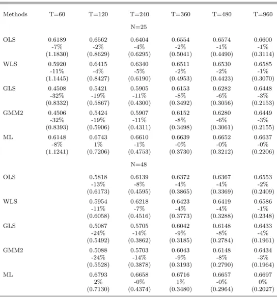
Consider first the case in which there is only one factor,K= 1. Table 1 provides the estimation results for the factor risk premium, γ1. For each of the estimation methods, we report the
aver-age estimate, ¯γ1, then the percentage error, (¯γ1−γ1)/γ1, and finally the root-mean-square error
(RMSE), the square root of PMm=1(ˆγ1(m)−γ1)2/M withM = 10,000. We begin by discussing the
results forN = 25 shown in the upper portion of Table 1.
Amsler and Schmidt (1985) note that when T is small, the maximum likelihood estimator is extremely volatile across simulations. We find this as well for the different test portfolios we consider. The ML results reported in the tables reflect truncation, as discussed earlier. Without truncation, the RMSE for the estimator of γ1 is theoretically unreliable. Nevertheless, it is of
interest to examine its value in the given simulation, which is 6.4 (13% bias) when T = 60, as compared to 1.12 (−8% bias) in Table 1. Truncation has little impact whenT = 120 and no effect for larger values of T. These are much longer samples than the 6 years examined by Amsler and Schmidt, but modest in relation to typical applications. GLS and GMM2 perform the best in terms of RMSE, with truncated ML (henceforth simply ML) not far behind whenT is at least 240. With a sample size as large asT = 960, all five of these estimators have about the same RMSE.
When N = 25 and T is at least 360, all methods have negative but fairly small percentage errors, implying that the estimators are slightly biased downward. This is expected for the two-pass estimators, given the well-known errors-in-variables (EIV) problem relating to estimation of the betas. Consistent with Proposition 4 and the positive value of γ1, the average ML estimate
across simulations exceeds the average GLS estimate. For example, when T = 360 the average is 0.664 for ML and 0.615 for GLS. As expected, the magnitude of the difference decreases as the sample size increases. When T = 120 or greater, ML has percentage errors of just 1% or less, the least among all the methods. The finding for ML is in keeping with Shanken’s demonstration that the ML estimator has a desirableN-consistency property, a sort of asymptotic unbiasedness, for fixed T. Panel B of Table 1 provides the results when N = 48. The qualitative conclusions are essentially the same as those for Panel A. Although the biases are minimal for ML, they are larger for the other estimators. This may be due to higher residual variances for the 48 industry portfolios, exacerbating the EIV problem.
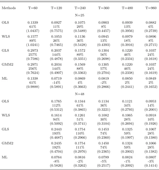
Table 2 provides the estimation results onγ0, the intercept in the expected return relation. As
was the case in estimating γ1, GLS and GMM2 are the best estimators of γ0 in terms of RMSE,
positive for the two-pass estimators and for GMM2 as well. The percentage biases are quite large, mainly due to the small magnitude ofγ0, as we discuss below. As earlier, ML has the least bias, at most 5% in magnitude whenT ≥240. To conserve space, we do not report the simulation standard deviations of the estimates in Tables 1 and 2. These are generally close to the RMSE’s, however. For example, withN = 48 and T = 240 the difference is about 0.015 for the GLS estimator of γ0
despite the large percentage bias of 110%.
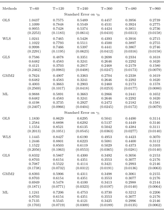
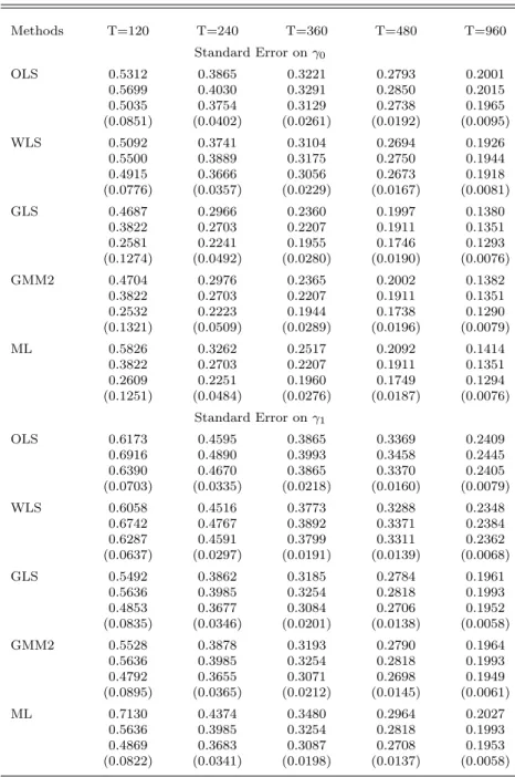
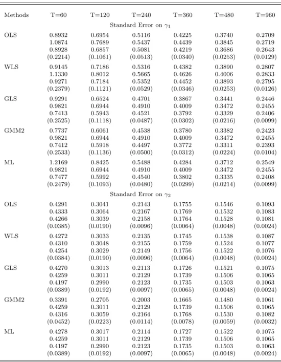
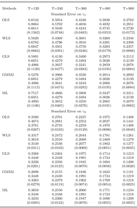
Next, we examine the standard errors of the estimates. For each estimator, Table 3 provides the RMSE followed by the asymptotic standard error evaluated at the true parameters, the average of the estimated asymptotic standard errors and, finally, the root-mean-square error of these estimated standard errors in parentheses. Results are given forN = 25 in Table 3a andN = 48 in Table 3b. Notice that the standard errors for γ0 and γ1 happen to be similar in magnitude. These standard
errors would be unaffected by changing the value of γ0, as the γ0 estimates would be shifted by
a fixed amount and the risk premium estimates would be unchanged. It also follows that the percentage bias in estimating γ0 would decline if its true value were increased in the simulations.
There are several important observations to be made about the standard errors. First, there is a tendency for the asymptotic standard errors of the OLS and WLS estimators to be a bit greater than RMSE when evaluated at the true parameter values, particularly in small samples. However, the asymptotic standard errors decline when evaluated at the second-pass estimates. In fact, this decline is observed for all estimators, though both standard errors are consistently below the RMSE for ML. For example, withN = 48 andT = 120, the OLS standard error for γ0 drops from 0.57 to
0.50, which is less than the RMSE of 0.53, whereas the standard errors for ML are 0.38 and 0.26, and RMSE is 0.58.
When T ≥ 360, the two asymptotic standard errors are fairly close to each other and to the RMSE’s of the estimates for the second-pass GLS/GMM2 estimators of the risk premium. The estimated second-pass GLS/GMM2 standard errors for the pricing intercept display more downward bias, however. The estimated ML standard errors have the worst bias; when T = 360, the RMSE is understated by as much as 10% for γ1 and 20% for γ0, withN = 48. The problem diminishes
as T increases but would be of particular concern if, contrary to typical practice, relatively short subperiods were to be used. Note that GLS, ML, and GMM2 all have the same asymptotic standard errors when evaluated at the true parameter values. Asymptotic equivalence was proven analytically for GLS and MLE in Shanken (1992), but apparently extends to our sequential GMM estimator as well when returns are iid normal.
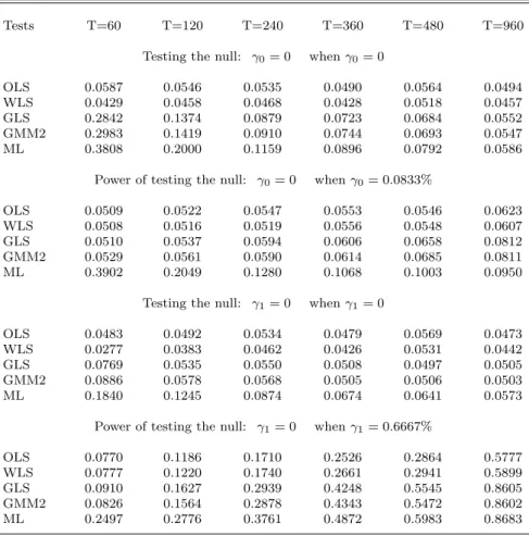
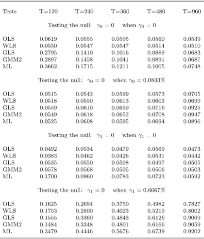
Now we consider “t-ratio” tests of the null hypothesis that a given parameter, either γ0 orγ1,
equals zero. All tests are two-sided, although one could argue for one-sided tests in a CAPM frame-work. The nominal size of the tests is set at 5% based on the asymptotic chi-squared distribution of the squared ratios. Table 4a (4b) provides both the actual rejection rates under the null and the empirical power of the test when N = 25 (N = 48). The traditional OLS test and the WLS test are well-specified under the null in most cases.
In testing γ0 = 0, the rejection rates are often large relative to 5% for the efficient estimators. Misspecification is greatest for the ML test andN = 48, with rejection probability 10% even when T = 480. This is due, in part, to the high kurtosis of ML (despite truncation) in the simulated data sets. Since the actual size of the tests often exceeds 5%, rejection rates under the alternative overstate the power of a 5% test. To overcome this problem, we compute the empirical power by using the upper 95th percentile of the 10,000 squared ratios simulated under the null. Although this is really an estimate of the population percentile, it should result in a better indication of the actual power of the test. In the limit, asT approaches infinity, power must approach one. However, even withT = 960, power is always less than 10% in the second panels of Tables 4a and 4b. Thus, we conclude that the test would have virtually no power in typical applications when the annualized value of γ0 is only 1%, a plausible differential a priori in the context of the zero-beta CAPM.
When testing the risk premium hypothesis γ1 = 0, all of the tests except ML have rejection
rates close to 5% under the null. Again, ML tends to reject too often, though the problem is not severe (rate <8%) whenT ≥360. The power of the tests is substantial when the annualized risk premium equals 8%, but does not exceed 0.5 until T ≥ 480. There are some power differences across estimation methods, with tests based on the OLS and WLS estimators exhibiting the lowest power and ML tests the highest.
It is interesting that the OLS version of the Fama-MacBeth method, used so extensively in the literature, is clearly dominated in terms of precision and power by the estimation methods that incorporate information about the covariance matrix of asset returns. A common view, generally unstated, is that while GLS-type estimators surely dominate in terms of asymptotic properties, the benefits will be lost when covariances have to be estimated. Our results for the one-factor model do not support this view. Moreover, it is surprising that adjusting the cross-sectional regressions for heteroskedasticity barely makes any difference in terms of bias, precision or power.22 Next, we 22An advantage for WLS could emerge when a large set of individual stocks or less-diversified portfolios is employed since heteroskedasticity is likely to be greater in that case. Typical applications employ a relatively small number of portfolios, however.
see whether these conclusions continue to hold in the context of a multifactor model.
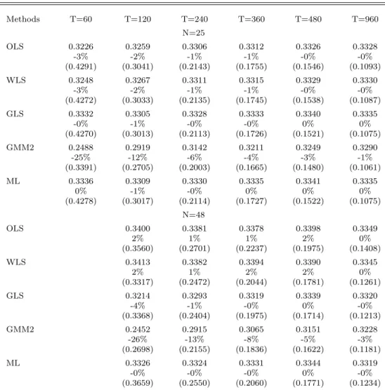
Consider now what happens when there are K = 3 factors. As earlier, we set the (truncated) ML estimates for all parameters equal to the GLS estimates when the magnitude of the ML estimate of any risk premium is more than twice that of the GLS estimate. Truncation is observed more often now, occurring a few times even when T = 960. Conclusions for the market risk premium estimators (results not shown) are qualitatively similar to those based on the one-factor model, except for a decline in the relative precision of ML. The variation in RMSE across estimators is less with the Fama-French factors, however, and biases are generally larger (except ML).
Table 5 reports estimation results for the book-to-market premium. Once again, ML has very little, if any, bias. GMM2 has the lowest RMSE, despite the fact that it is the most biased estimator. Differences in RMSE are minor whenN = 25, except for the smallest values of T. A bit more variation in RMSE is observed when N = 48, ranging from 0.18 for GMM2 to 0.22 for OLS when T = 360. Results for the size premium and the zero-beta intercept (not shown) are similar to those for book-to-market.
We have also examined simulation results for standard errors and t-ratios in the three-factor model. All of the findings are summarized, though only results for the market and book-to-market premia are shown (Tables 6a and 6b). The rest are available on request. As in Tables 3a and 3b, we find downward bias in the estimated standard errors for γ0 using GLS and GMM2, with the
worst bias using ML. The estimated ML standard errors for γ1 are too low as well, by as much as 15% when T = 360, and the ML RMSE’s are particularly high with N = 25. The behavior of the t-ratios for γ0 and γ1 is also fairly similar to that observed earlier. The estimated standard errors for the size and book-to-market premia are generally quite close to the RMSE’s and to the true asymptotic values for all estimators. Likewise, the tests for size and book-to-market premia are typically well specified under the null, with GMM2 sometimes displaying a slight tendency to underreject.
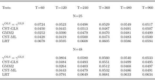
We now turn to tests of the maintained assumption of an exact linear relation between expected return and beta, as given in (2). Tables 7 and 8 examine the actual size of the various (nominal) 5% level tests of this linear specification for the one and three-factor models, respectively. The rejection rates are based on simulations in which the expected return relation holds, with the positive parameter values described earlier. The cross-sectional tests both perform quite well for all models except whenT is very small. GMM2 over-rejects in tests of the three-factor model. LRT displays a more systematic tendency to over-reject somewhat, with probabilities ranging from 0.06
to 0.09 when T = 360. Finally, our univariate specification test based on the difference between OLS and GLS estimators is fairly well specified for samples this large.
In addition to the multivariate tests, we have examined the traditional Fama-MacBeth univari-ate test based on thet-ratio for an additional cross-sectional variable. This experiment is conducted forN = 25 under the CAPM null hypothesis. The additional independent variable is taken to be the (time-series) average book-to-market ratio for each portfolio, as reported in Fama and French (1993). The rejection rates (not shown) are close to 5% for OLS and WLS at all sample sizes. The GLS test rejects too often in small samples. The rejection rate declines to 6.5% forT = 360, but is still 6% for T as large as 960.
5.2 Results when the linear expected return model is misspecified
Like the asymptotic results on estimation in Shanken (1992) and Jagannathan and Wang (1998), our simulations thus far have assumed that the linear expected return model is correctly specified. Now we allow for the possibility of deviations from the model. Of course, there are many ways in which the expected return restriction could be violated. We consider two cases of interest, both of which entail estimation and testing of a misspecified zero-beta CAPM. In each case, pricing errors are added to the CAPM expected returns withγ0 = 0.0833% and γ1= 0.6667%, as earlier. When N = 25, the pricing errors are taken to be the Fama-French estimates of the excess-return alphas for the size/book-to-market portfolios. WhenN = 48, we randomly draw a CAPM deviation from a normal distribution with mean zero and standard deviation 0.1667% or 2% annualized. In each case, the deviations are taken to be fixed over time and thus betas and covariance parameters are unaffected.
As discussed in Section 2, when using the Fama-MacBeth method, the implied coefficients in the single-factor expected return relation are determined by projecting the true expected return vector on the univariate beta vector and a constant vector. The projection varies with the weighting matrix employed. ForN = 25, the true parameters under OLS, WLS, and GLS are 1.03%, 0.76%, and 1.01%, respectively, for γ0 and −0.06%, 0.14%, and −0.25% for γ1. Thus, introducing the
Fama-French alphas largely eliminates the correlation between expected returns and market betas. This is presumably driven by the relatively high (low) betas and negative (positive) alphas of low (high) book-to-market stocks. When N = 48, the projection coefficients are γ0 = 0.22%, 0.28%,
0.52%, and γ1 = 0.55%, 0.48%, 0.20%, for OLS, WLS, and GLS, respectively. In this case, the
random nature of the pricing errors.
As expected, when we simulate the misspecified models, the average estimates (not shown) ap-proach the corresponding theoretical projection parameters asT increases. Less clear is the impact of misspecification on the standard errors of the estimates. Table 9 reports, forN = 25, the RMSE of each estimator followed by two sets of asymptotic standard errors. The first set is evaluated at the true parameter values, ignoring model misspecification and then taking it into account. The second pair consists of the corresponding simulation averages of the estimated asymptotic standard errors. Interestingly, we find that the asymptotic adjustment for model misspecification increases the standard errors, but minimally in this context. For example, when T = 360, the estimated standard error for the GLS estimator ofγ1 increases from 0.34 to 0.37. Similar results (not shown)
are obtained whenN = 48.
Tests of the linear expected return relation for N = 25 and N = 48 are reported in Table 10. Since the CST’s appear to have the appropriate size based on the earlier analysis, the rejection rates for these tests can be viewed as estimates of the power of a 5% test. We see that the multivariate CST’s have substantial power against both alternatives when T ≥240. The power of the coefficient-based test (which may be overstated slightly in small samples) is lower, particularly forN = 48.
5.3 Conditional heteroscedasticity
Thus far, returns have been assumed to be distributed iid normal in our simulations. Now we examine the sensitivity of estimation and test results to the joint normality assumption. As Kan and Zhou (2003) show, a multivariate t-distribution with 8 degrees of freedom fits the data well.23
In addition, under thet assumption, the residual variance depends on the factors, and so contem-poraneous conditional heteroscedasticity is introduced. We generate the data as before, except that the joint normality assumption for the factors and returns is replaced by the joint tassumption.
Table 11 reports estimation results for γ1. The results are fairly robust to the assumed
con-ditional heteroscedasticity when T ≥ 360, but some small effects are observed. For example, compared to Table 1, the GLS estimator is slightly more biased and its RMSE slightly higher in Table 11, while the OLS RMSE declines a bit for N = 25. Also, MLE now has a negative bias,
23Here, we refer to the unconditional distribution of the data. Exploring the behavior of conditional tests when the variance of returns is allowed to change is beyond the scope of this paper, but an important topic that we hope to address in future work.
but it is less than 5% of the true value for reasonable sample sizes. The cross-sectional F tests of expected return linearity, which performed quite well under homoskedasticity, continue to display the proper size (close to 5%) under conditional heteroskedasticity (results not shown).
6
Application
The standard excess-return time-series formulation of the Fama and French (1993) three-factor model constrains the alphas to equal zero, implicitly assuming that the zero-beta rate equals the riskless rate and the factor risk premia equal the corresponding factor means. As noted in Shanken and Weinstein (1990), the latter restriction is implied whenever the factors are spread portfolio returns. It is well-known that the constrained model can be evaluated by the Gibbons, Ross and Shanken (1989) test or, if the normality assumption is a concern, by methods that allow for conditional heteroskedasticity, as in MacKinlay and Richardson (1991) and Shanken (1990). In this section, we relax the usual pricing restrictions and apply the earlier cross-sectional regression methods in an analysis of the Fama-French model. This can be likened, in some respects, to Fama and MacBeth’s (1973) analysis of the original Sharpe-Lintner CAPM.
The empirical factor model is:
Rit−rf t =αi+βi1(fM,t−rf t) +βi2fSM B,t+βi3fHM L,t+²it, (46)
where fM is the market return factor, fSM B is the small-big return spread, fHM L is the high-low return spread, and rf t is the 30-day T-bill rate. The Rit’s are the test asset returns on the 25
stock portfolios formed on size and book-to-market. The following asset pricing relationship is of interest,
H0: E(Rit−rf t) =γ0+γ1βi1+γ2βi2+γ3βi3, (47)
whereγ1, γ2, and γ3 are the risk premium parameters, andγ0 is the excess zero-beta rate.
Table 12 reports the results. The first column indicates which of the five estimation methods is used. The next four columns provide estimation results for each of the risk-return parameters. The point estimate is given with its standard error in parentheses, both in percent. The last column contains, for each second-pass estimation method, a chi-squared test of significance comparing the cross-sectional regression estimates of the risk-return parameters to the usual time-series means (andγ0= 0).