Data assimilation: the Schrödinger
perspective
Article
Accepted Version
Reich, S. (2019) Data assimilation: the Schrödinger
perspective. Acta Numerica, 28. pp. 635-711. ISSN 0962-4929
doi: https://doi.org/10.1017/S0962492919000011 Available at
http://centaur.reading.ac.uk/90171/
It is advisable to refer to the publisher’s version if you intend to cite from the
work. See
Guidance on citing
.
Published version at: http://dx.doi.org/10.1017/S0962492919000011
To link to this article DOI: http://dx.doi.org/10.1017/S0962492919000011
Publisher: Cambridge University Press
All outputs in CentAUR are protected by Intellectual Property Rights law,
including copyright law. Copyright and IPR is retained by the creators or other
copyright holders. Terms and conditions for use of this material are defined in
the
End User Agreement
.
CentAUR
Central Archive at the University of Reading
Reading’s research outputs online
Data Assimilation: The Schr¨
odinger Perspective
Sebastian Reich
∗May 2, 2019
Abstract
Data assimilation addresses the general problem of how to combine model-based predictions with par-tial and noisy observations of the process in an optimal manner. This survey focuses on sequenpar-tial data assimilation techniques using probabilistic particle-based algorithms. In addition to surveying recent de-velopments for discrete- and continuous-time data assimilation, both in terms of mathematical foundations and algorithmic implementations, we also provide a unifying framework from the perspective of coupling of measures, and Schr¨odinger’s boundary value problem for stochastic processes in particular.
1
Introduction
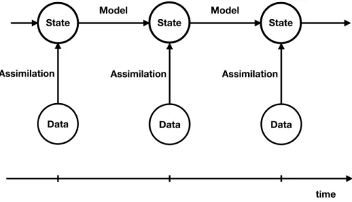
This survey focuses on sequential data assimilation techniques for state and parameter estimation in the context of discrete- and continuous-time stochastic diffusion processes. See Figure 1. The field itself is well established (Evensen 2006, S¨arkk¨a 2013, Law, Stuart and Zygalakis 2015, Reich and Cotter 2015, Asch, Bocquet and Nodet 2017), but is also undergoing continuous development due to new challenges arising from emerging application areas such as medicine, traffic control, biology, cognitive sciences and geosciences.
Data assimilation is typically formulated within a Bayesian framework in order to combine partial and noisy observations with model predictions and their uncertainties with the goal of adjusting model states and model parameters in an optimal manner. In the case of linear systems and Gaussian distributions, this task leads to the celebrated Kalman filter (S¨arkk¨a 2013) which even today forms the basis of a number of popular data assimilation schemes and which has given rise to the widely used ensemble Kalman filter (Evensen 2006). Contrary to standard sequential Monte Carlo methods (Doucet, de Freitas and (eds.) 2001, Bain and Crisan 2008), the ensemble Kalman filter does not provide a consistent approximation to the sequential filtering problem, while being applicable to very high-dimensional problems. This and other advances have widened the scope of sequential data assimilation and have led to an avalanche of new methods in recent years.
In this review we will focus on probabilistic methods (in contrast to data assimilation techniques based on optimisation, such as 3DVar and 4DVar (Evensen 2006, Law et al. 2015)) in the form of sequential particle methods. The essential challenge of sequential particle methods is to convert a sample of M particles from a filtering distribution at time tk into M samples from the filtering distribution at time tk+1 without having
access to the full filtering distributions. It will also often be the case in practical applications that the sample size will be small to moderate in comparison to the number of variables we need to estimate.
Sequential particle methods can be viewed as a special instance of interacting particle systems (del Moral 2004). We will view such interacting particle systems in this review from the perspective of approximating a cer-tain boundary value problem in the space of probability measures, where the boundary conditions are provided by the underlying stochastic process, the data, and Bayes’ theorem. This point of view leads naturally to optimal transportation (Villani 2003, Reich and Cotter 2015) and, more importantly for this review, to Schr¨odinger’s problem (F¨ollmer and Gantert 1997, Leonard 2014, Chen, Georgiou and Pavon 2014), as formulated first by Erwin Schr¨odinger in the form of a boundary value problem for Brownian motion (Schr¨odinger 1931).
This paper has been written with the intention of presenting a unifying framework for sequential data assimilation using coupling of measure arguments provided through optimal transportation and Schr¨odinger’s problem. We will also summarise novel algorithmic developments that were inspired by this perspective. Both discrete- and continuous-time processes and data sets will be covered. While the primary focus is on state estimation, the presented material can be extended to combined state and parameter estimation. See Remark 2.2 below.
∗Department of Mathematics, University of Potsdam & University of Reading,[email protected]
State State State Model Model Data Assimilation Data Assimilation Data Assimilation time
Figure 1: Schematic illustration of sequential data assimilation, where model states are propagated forward in time under a given model dynamics and adjusted whenever data become available at discrete instances in time. In this paper, we look at a single transition from a given model state conditioned on all the previous and current data to the next instance in time, and its adjustment under the assimilation of the new data then becoming available.
Remark 1.1. We will primary refer to the methods considered in the survey as particle or ensemble methods
instead of the widely used notion of sequential Monte Carlo methods. We will also use the notions of particles, samples and ensemble members synonymously. Since the ensemble size, M, is generally assumed to be small to moderate relative to the number of variables of interest, we will focus on robust but generally biased particle methods.
1.1
Overall organisation of the paper
This survey consists of four main parts. We start Section 2 by recalling key mathematical concepts of sequential data assimilation when the data become available at discrete instances in time. Here the underlying dynamic models can be either continuous (that is, is generated by a stochastic differential equation) or discrete-in-time. Our initial review of the problem will lead to the identification of three different scenarios of performing sequential data assimilation, which we denote by (A), (B) and (C). While the first two scenarios are linked to the classical importance resampling and optimal proposal densities for particle filtering (Doucet et al. 2001), scenario (C) builds upon an intrinsic connection to a certain boundary value problem in the space of joint probability measures first considered by Erwin Schr¨odinger (Schr¨odinger 1931).
After this initial review, the remaining parts of Section 2 provide more mathematical details on prediction in Section 2.1, filtering and smoothing in Section 2.2, and the Schr¨odinger approach to sequential data assimilation in Section 2.3. The modification of a given Markov transition kernel via a twisting function will arise as a crucial mathematical construction and will be introduced in Sections 1.2 and 2.1. The next major part of the paper, Section 3, is devoted to numerical implementations of prediction, filtering and smoothing, and the Schr¨odinger approach as relevant to scenarios (A)–(C) introduced earlier in Section 2. More specifically, this part will cover the ensemble Kalman filter and its extensions to the more general class of linear ensemble transform filters as well as the numerical implementation of the Schr¨odinger approach to sequential data assimilation using the Sinkhorn algorithm (Sinkhorn 1967, Peyre and Cuturi 2018). Discrete-time stochastic systems with additive Gaussian model errors and stochastic differential equations with constant diffusion coefficient serve as illustrating examples throughout both Sections 2 and 3.
Sections 2 and 3 are followed by two sections on the assimilation of data that arrive continuously in time. In Section 4 we will distinguish between data that are smooth as a function of time and data which have been perturbed by Brownian motion. In both cases, we will demonstrate that the data assimilation problem can be reformulated in terms of so-called mean-field equations, which produce the correct conditional marginal distributions in the state variables. In particular, in Section 4.2 we discuss the feedback particle filter of Yang, Mehta and Meyn (2013) in some detail. The final section of this review, Section 5, covers numerical approximations to these mean-field equations in the form of interacting particle systems. More specifically, the continuous-time ensemble Kalman–Bucy and numerical implementations of the feedback particle filter will be covered in detail. It will be shown in particular that the numerical implementation of the feedback particle filter can be achieved naturally via the approximation of an associated Schr¨odinger problem using the Sinkhorn algorithm.
In the appendices we provide additional background material on mesh-free approximations of the Fokker– Planck and backward Kolmogorov equations (Appendix A), on the regularised St¨ormer–Verlet time-stepping methods for the hybrid Monte Carlo method, applicable to Bayesian inference problems over path spaces (Appendix B), on the ensemble Kalman filter (Appendix C), and on the numerical approximation of forward– backward stochastic differential equations (SDEs) (Appendix D).
1.2
Summary of essential notations
We typically denote the probability density function (PDF) of a random variableZ byπ. Realisations ofZ will be denoted byz=Z(ω).
Realisations of a random variable can also be continuous functions/paths, in which case the associated probability measure on path space is denoted by Q. We will primarily consider continuous functions over the unit time interval and denote the associated random variable by Z[0,1] and its realisations Z[0,1](ω) by z[0,t].
The restriction of Z[0,1] to a particular instance t∈ [0,1] is denoted by Zt with marginal distribution πt and
realisationszt=Zt(ω).
For a random variable Z having only finitely many outcomeszi,i= 1, . . . , M, with probabilitiesp
i, that is,
P[Z(ω) =zi] =p i,
we will work with either the probability vectorp= (p1, . . . , pM)Tor the empirical measure
π(z) =
M
X
i=1
piδ(z−zi),
whereδ(·) denotes the standard Dirac delta function. We use the shorthand
π[f] =
Z
f(z)π(z) dz
for the expectation of a functionf under a PDFπ. Similarly, integration with respect to a probability measure
Q, not necessarily absolutely continuous with respect to Lebesgue, will be denoted by
Q[f] =
Z
f(z)Q(dz).
The notationE[f] is used if we do not wish to specify the measure explicitly.
The PDF of a Gaussian random variable, Z, with mean ¯z and covariance matrix B will be abbreviated by n(z; ¯z, B). We also writeZ ∼N(¯z, B).
Let u∈RN, thenD(u)∈RN×N denotes the diagonal matrix with entries (D(u))ii =ui,i= 1, . . . , N. We
also denote theN×1 vector of ones by1N = (1, . . . ,1)T∈RN.
A matrix P ∈ RL×M is called bi-stochastic if all its entries are non-negativ, which we will abbreviate by
P ≥0, and L X l=1 qli=p0, M X i=1 qli=p1,
where bothp1∈RL andp0∈RM are probability vectors. A matrixQ∈RM×M defines a discrete Markov chain
if all its entries are non-negative and
L
X
l=1
The Kullback–Leibler divergence between two bi-stochastic matricesP ∈RL×M andQ∈RL×M is defined by KL (P||Q) :=X l,j pljlog plj qlj .
Here we have assumed for simplicity thatqlj>0 for all entries of Q. This definition extends to the Kullback–
Leibler divergence between two discrete Markov chains.
The transition probability going from statez0at timet= 0 to statez1at timet= 1 is denoted byq+(z1|z0).
Hence, given an initial PDFπ0(z0) att= 0, the resulting (prediction or forecast) PDF at timet= 1 is provided
by
π1(z1) :=
Z
q+(z1|z0)π0(z0) dz0. (1)
Given a twisting functionψ(z)>0, the twisted transition kernelqψ+(z1|z0) is defined by
q+ψ(z1|z0) :=ψ(z1)q+(z1|z0)ψb(z0)−1 (2) provided b ψ(z0) := Z q+(z1|z0)ψ(z1) dz1 (3)
is non–zero for allz0. See Definition 2.8 for more details.
If transitions are characterised by a discrete Markov chainQ+∈RM, then a twisted Markov chain is provided
by
Qu+ =D(u)Q+D(v)−1
for given twisting vectoru∈RM with positive entries ui, that is,u >0, and the vector v∈RM determined by
v= (D(u)Q+)T1M.
The conditional probability of observing y given z is denoted by π(y|z) and the likelihood of z given an observedyis abbreviated byl(z) =π(y|z). We will also use the abbreviations
b
π1(z1) =π1(z1|y1)
and
b
π0(z0) =π0(z0|y1)
to denote the conditional PDFs of a process at timet= 1 given data at timet= 1 (filtering) and the conditional PDF at timet= 0 given data at timet= 1 (smoothing), respectively. Finally, we also introduce the evidence
β :=π1[l] =
Z
p(y1|z1)π1(z1)dz1
of observing y1 under the given model as represented by the forecast PDF (1). A more precise definition of
these expressions will be given in the following section.
2
Mathematical foundation of discrete-time DA
Let us assume that we are given partial and noisy observations yk, k = 1, . . . , K, of a stochastic process in
regular time intervals of lengthT = 1. Given a likelihood functionπ(y|z), a Markov transition kernelq+(z0|z)
and an initial distribution π0, the associated prior and posterior PDFs are given by
π(z0:K) :=π0(z0) K Y k=1 q+(zk|zk−1) (4) and π(z0:K|y1:K) := π0(z0)QKk=1π(yk|zk)q+(zk|zk−1) π(y1:K) , (5)
respectively (Jazwinski 1970, S¨arkk¨a 2013). While it is of broad interest to approximate the posterior or smoothing PDF (5), we will focus on the recursive approximation of the filtering PDFsπ(zk|y1:k) using sequential
Problem 2.1. We have M equally weighted Monte Carlo samples zi
k−1,i= 1, . . . , M, from the filtering PDF
π(zk−1|y1:k−1)at timet=k−1available and we wish to produceM equally weighted samples from the filtering
PDFπ(zk|y1:k)at timet=khaving access to the transition kernelq+(zk|zk−1)and the likelihoodπ(yk|zk)only.
Since the computational task is exactly the same for all indicesk≥1, we simply setk= 1throughout this paper.
We introduce some notations before we discuss several possibilities of addressing Problem 2.1. Since we do not have direct access to the filtering distribution at time k= 0, the PDF att0 becomes
π0(z0) := 1 M M X i=1 δ(z0−z0i), (6)
whereδ(z) denotes the Dirac delta function andzi
0,i= 1, . . . , M, areM given Monte Carlo samples representing
the actual filtering distribution. Recall that we abbreviate the resulting filtering PDFπ(z1|y1) att= 1 byπb1(z1)
and the likelihoodπ(y1|z1) byl(z1). Because of (1), the forecast PDF is given by
π1(z1) = 1 M M X i=1 q+(z1|z0i) (7)
and the filtering PDF at timet= 1 by
b π1(z1) := l(z1)π1(z1) π1[l] = 1 π1[l] 1 M M X i=1 l(z1)q+(z1|zi0) (8)
according to Bayes’ theorem.
Remark 2.2. The normalisation constantπ(y1:K)in(5), also called the evidence, can be determined recursively
using π(y1:k) =π(y1:k−1) Z π(yk, zk−1)π(zk−1|y1:k−1)dzk−1 =π(y1:k−1) Z Z π(yk|zk)q+(zk|zk−1)π(zk−1|y1:k−1)dzk−1dzk =π(y1:k−1) Z π(yk|zk)π(zk|y1:k−1)dzk (9)
(S¨arkk¨a 2013, Reich and Cotter 2015). Since, as for the state estimation problem, the computational task is the same for each indexk≥1, we simply setk= 1and formally use π(y1:0)≡1. We are then left with
β:=π1[l] = 1 M M X i=1 Z l(z1)q+(z1|z0i) dz1 (10)
within the setting of Problem 2.1 and β is a shorthand for π(y1). If the model depends on parameters, λ,
or different models are to be compared, then it is important to evaluate the evidence (10) for each parameter valueλor model, respectively. More specifically, ifq+(z1|z0;λ), thenβ=β(λ)in(10)and larger values ofβ(λ)
indicate a better fit of the transition kernel to the data for that parameter value. One can then perform Bayesian parameter inference based upon appropriate approximations to the likelihood π(y1|λ) =β(λ)and a given prior
PDFπ(λ). The extension to the complete data sety1:K,K >1, is straightforward using (9)and an appropriate
data assimilation algorithm, that is, algorithms that can tackle problem 2.1 sequentially.
Alternatively, one can treat a combined state–parameter estimation problem as a particular case of problem 2.1 by introducing the extended state variable(z, λ)and augmented transition probabilitiesZ1∼q+(·|z0, λ0)and
P[Λ1=λ0] = 1. The state augmentation technique allows one to extend all approaches discussed in this paper
for Problem 2.1 to combined state–parameter estimation.
See Kantas, Doucet, Singh, Maciejowski and Chopin (2015) for a detailed survey of the topic of combined state and parameter estimation.
The filtering distributionbπ1 at timet= 1 implies a smoothing distribution at timet= 0, which is given by b π0(z0) := 1 β Z l(z1)q+(z1|z0)π0(z0) dz1= 1 M M X i=1 γiδ(z 0−z0i) (11) with weights γi := 1 β Z l(z1)q+(z1|z0i) dz1. (12)
It is important to note that the filtering PDFπb1 can be obtained fromπb0using the transition kernels
b q+(z1|zi0) := l(z1)q+(z1|zi0) β γi , (13) that is, b π1(z1) = 1 M M X i=1 b q+(z1|z0i)γ i .
See Figure 2 for a schematic illustration of these distributions and their mutual relationships.
Remark 2.3. The modified transition kernel (13)can be seen as a particular instance of a twisted transition
kernel (2) withψ(z) =l(z)/β andψb(zi
0) =γi. Such twisting kernels will play a prominent role in this survey,
not only in the context of optimal proposals (Doucet et al. 2001, Arulampalam, Maskell, Gordon and Clapp 2002) but also in the context of the Schr¨odinger approach to data assimilation, that is, to scenario (C) below.
The following scenarios of how to tackle Problem 2.1, that is, how to produce the desired samples zbi 1, i =
1, . . . , M, from the filtering PDF (8), will be considered in this paper.
Definition 2.4. We define the following three scenarios of how to tackle Problem 2.1.
(A) We first produces samples,zi
1, from the forecast PDF π1 and then transform those samples into samples,
b
zi
1, fromπb1. This can be viewed as introducing a Markov transition kernelq1(zb1|z1)with the property that
b
π1(zb1) =
Z
q1(zb1|z1)π1(z1) dz1. (14)
Techniques from optimal transportation can be used to find appropriate transition kernels (Villani 2003, Villani 2009, Reich and Cotter 2015).
(B) We first produce M samples from the smoothing PDF (11) via resampling with replacement and then sample from bπ1 using the smoothing transition kernels(13). The resampling can be represented in terms
of a Markov transition matrix Q0∈RM×M such that
γ=Q0p.
Here we have introduced the associated probability vectors γ=γM1, . . . ,γMMT∈RM, p= 1 M, . . . , 1 M T ∈RM. (15)
Techniques from optimal transport will be explored to find such Markov transition matrices in Section 3. (C) We directly seek Markov transition kernels q∗
+(z1|z0i),i= 1, . . . , M, with the property that
b π1(z1) = 1 M M X i=1 q+∗(z1|zi0) (16)
and then draw a single sample, bzi
1, from each kernel q+∗(z1|zi0). Such kernels can be found by solving a
⇡
0
Prediction⇡
1
Filteringb
⇡
1b
⇡
0
Smoothing Optimal control Data Timet
= 0
t
= 1
Schrödingery
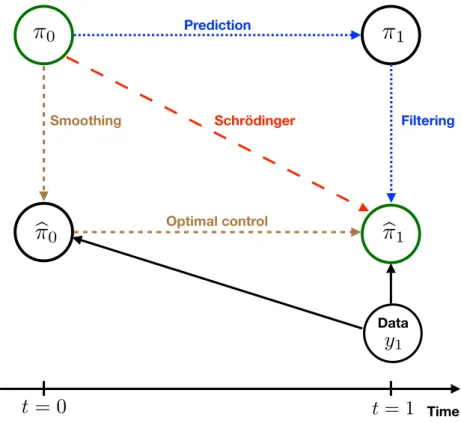
1Figure 2: Schematic illustration of a single data assimilation cycle. The distribution π0 characterises the
distribution of states conditioned on all observations up to and including t0, which we set here to t = 0 for
simplicity. The predictive distribution at timet1= 1, as generated by the model dynamics, is denoted by π1.
Upon assimilation of the data y1 and application of Bayes’ formula, one obtains the filtering distribution bπ1.
The conditional distribution of states at timet0conditioned on all the available data includingy1is denoted by
b
π0. Control theory provides the adjusted model dynamics for transformingπb0intoπb1. Finally, the Schr¨odinger
problem links π0 and πb1 in the form of a penalised boundary value problem in the space of joint probability
measures. Data assimilation scenario (A) corresponds to the dotted lines, scenario (B) to the short-dashed lines, and scenario (C) to the long-dashed line.
Scenario (A) forms the basis of the classical bootstrap particle filter (Doucet et al. 2001, Liu 2001, Bain and Crisan 2008, Arulampalam et al. 2002) and also provides the starting point for many currently used ensemble-based data assimilation algorithms (Evensen 2006, Reich and Cotter 2015, Law et al. 2015). Scenario (B) is also well known in the context of particle filters under the notion of optimal proposal densities (Doucet et al. 2001, Arulampalam et al. 2002, Fearnhead and K¨unsch 2018). Recently there has been a renewed interest in scenario (B) from the perspective of optimal control and twisting approaches (Guarniero, Johansen and Lee 2017, Heng, Bishop, Deligiannidis and Doucet 2018, Kappen and Ruiz 2016, Ruiz and Kappen 2017). Finally, scenario (C) has not yet been explored in the context of particle filters and data assimilation, primarily because the required kernels q+∗ are typically not available in closed form or cannot be easily sampled from. However,
as we will argue in this paper, progress on the numerical solution of Schr¨odinger’s problem (Cuturi 2013, Peyre and Cuturi 2018) turns scenario (C) into a viable option in addition to providing a unifying mathematical framework for data assimilation.
We emphasise that not all existing particle methods fit into these three scenarios. For example, the methods put forward by Van Leeuwen (2015) are based on proposal densities which attempt to overcome limitations of scenario (B) and which lead to less variable particle weights, thus attempting to obtain particle filter implemen-tations closer to what we denote here as scenario (C). More broadly speaking, the exploration of alternative proposal densities in the context of data assimilation has started only recently. See, for example, Vanden-Eijnden and Weare (2012), Morzfeld, Tu, Atkins and Chorin (2012), Van Leeuwen (2015), Llopis, Kantas, Beskos and Jasra (2018), and van Leeuwen, K¨unsch, Nerger, Potthast and Reich (2018).
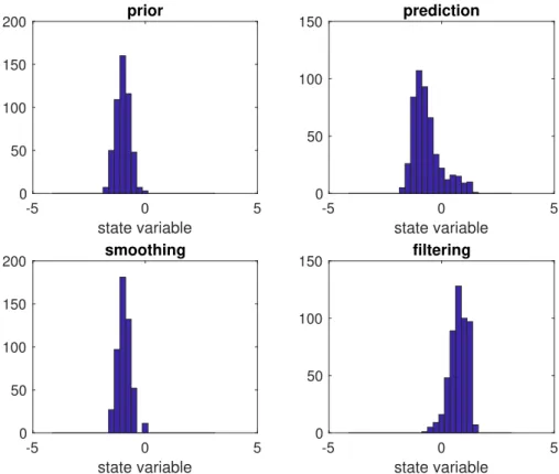
prior
-1 -0.5 0 0.5 1space
0 0.02 0.04 0.06 0.08 0.1 -4 -2 0 2 4space
0 0.1 0.2 0.3 0.4 0.5prediction
smoothing
-1 -0.5 0 0.5 1space
0 0.05 0.1 0.15 0.2 -4 -2 0 2 4space
0 0.5 1 1.5filtering
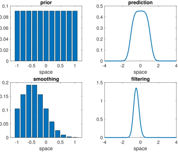
Figure 3: The the initial PDFπ0, the forecast PDF π1, the filtering PDFbπ1, and the smoothing PDFπb0 for a
simple Gaussian transition kernel.
The accuracy of an ensemble–based data assimilation method can be characterised in terms of its effective sample sizeMeff (Liu 2001). The relevant effective sample size for scenario (B) is, for example, given by
Meff = M2 PM i=1(γi)2 = 1 kγk2.
We find that M ≥ Meff ≥ 1 and the accuracy of a data assimilation step decreases with decreasing Meff,
that is, the convergence rate 1/√M of a standard Monte Carlo method is replaced by 1/√Meff (Agapiou,
Papaspipliopoulos, Sanz-Alonso and Stuart 2017). Scenario (C) offers a route around this problem by bridging
π0withbπ1directly, that is, solving the Schr¨odinger problem delivers the best possible proposal densities leading
to equally weighted particles without the need for resampling.1
Example 2.5. We illustrate the three scenarios with a simple example. The prior samples are given byM = 11
equally spaced particleszi
0∈Rfrom the interval[−1,1]. The forecast PDF π1 is provided by
π1(z) = 1 M M X i=1 1 (2π)1/2σexp − 1 2σ2(z−z i 0)2
with varianceσ2= 0.1. The likelihood function is given by
π(y1|z) = 1 (2πR)1/2exp − 1 2R(y1−z)2
1The kernel (13) is called the optimal proposal in the particle filter community. However, the kernel (13) is suboptimal in the
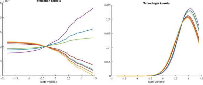
-2 -1.5 -1 -0.5 0 0.5 1 1.5 space 0 0.5 1 1.5 2
2.5 optimal control proposals
-2 -1.5 -1 -0.5 0 0.5 1 1.5 space 0 0.5 1 1.5 2 2.5 Schroedinger proposal
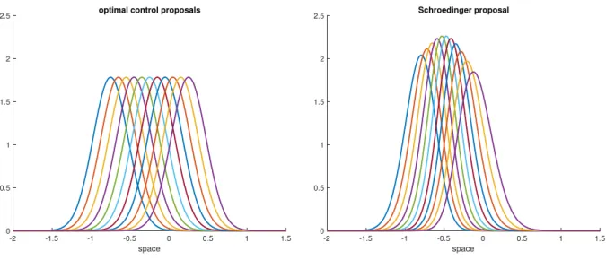
Figure 4: Left panel: The transition kernels (17) for theM = 11 different particleszi
0. These correspond to the
optimal control path in figure 2. Right panel: The corresponding transitions kernels, which lead directly from
π0 toπb1. These correspond to the Schr¨odinger path in figure 2. Details of how to compute these Schr¨odinger
transition kernels,q∗
+(z1|z0i), can be found in Section 3.4.1.
withR= 0.1 andy1=−0.5. The implied filtering and smoothing distributions can be found in Figure 3. Since
b
π1 is in the form of a weighted Gaussian mixture distribution, the Markov chain leading from bπ0 tobπ1 can be
stated explicitly, that is,(13)is provided by
b q+(z1|z0i) = 1 (2π)1/2σbexp − 1 2σb2(¯z i 1−z1)2 (17) with b σ2=σ2− σ4 σ2+R, z¯ i 1=z0i− σ2 σ2+R(z i 0−y1).
The resulting transition kernels are displayed in Figure 4 together with the corresponding transition kernels for the Schr¨odinger approach, which connectsπ0 directly withπb1.
Remark 2.6. It is often assumed in optimal control or rare event simulations arising from statistical mechanics
thatπ0 in(4)is a point measure, that is, the starting point of the simulation is known exactly. See, for example,
Hartmann, Richter, Sch¨utte and Zhang (2017). This corresponds to (6) with M = 1. It turns out that the associated smoothing problem becomes equivalent to Schr¨odinger’s problem under this particular setting since the distribution at t= 0 is fixed.
The remainder of this section is structured as follows. We first recapitulate the pure prediction problem for discrete-time Markov processes and continuous-time diffusion processes, after which we discuss the filtering and smoothing problem for a single data assimilation step as relevant for scenarios (A) and (B). The final subsection is devoted to the Schr¨odinger problem (Leonard 2014, Chen et al. 2014) of bridging the filtering distribution,
π0, at t= 0 directly with the filtering distribution,bπ1, at t= 1, thus leading to scenario (C).
2.1
Prediction
We assume under the chosen computational setting that we have access toM sampleszi
0∈RNz,i= 1, . . . , M,
from the filtering distribution at t = 0. We also assume that we know (explicitly or implicitly) the forward transition probabilities, q+(z1|z0i), of the underlying Markovian stochastic process. This leads to the forecast
PDF, π1, as given by (7).
Before we consider two specific examples, we introduce two concepts related to the forward transition kernel which we will need later in order to address scenarios (B) & (C) from Definition 2.4.
We first introduce the backward transition kernelq−(z0|z1), which is defined via the equation
q−(z0|z1)π1(z1) =q+(z1|z0)π0(z0).
Note thatq−(z0|z1) as well asπ0are not absolutely continuous with respect to the underlying Lebesque measure,
that is, q−(z0|z1) = 1 M M X i=1 q+(z1|z0i) π1(z1) δ(z0−z0i). (18)
The backward transition kernelq−(z1|z0) reverses the prediction process in the sense that
π0(z0) =
Z
q−(z0|z1)π1(z1) dz1.
Remark 2.7. Let us assume that the detailed balance
q+(z1|z0)π(z0) =q+(z0|z1)π(z1)
holds for some PDFπ and forward transition kernelq+(z1|z0). Thenπ1=πforπ0=π(invariance of π) and
q−(z0|z1) =q+(z1|z0).
We next introduce a class of forward transition kernels using the concept of twisting (Guarniero et al. 2017, Heng et al. 2018), which is an application of Doob’s H-transform technique (Doob 1984).
Definition 2.8. Given a non-negative twisting function ψ(z1) such that the modified transition kernel (2) is
well-defined, one can define the twisted forecast PDF
π1ψ(z1) := 1 M M X i=1 q+ψ(z1|zi0) = 1 M M X i=1 ψ(z1) b ψ(zi 0) q+(z1|z0i). (19)
The PDFsπ1 andπ1ψ are related by
π1(z1) πψ1(z1) = PM i=1q+(z1|z0i) PM i=1 ψ(z1) b ψ(zi 0) q+(z1|zi0) . (20)
Equation (20) gives rise to importance weights
wi∝ π1(z i 1) π1ψ(zi 1) (21) for sampleszi
1=Z1i(ω) drawn from the twisted forecast PDF, that is,
Zi 1∼q ψ +(· |zi0) and π1(z)≈ 1 M M X i=1 wiδ(z−zi 1)
in a weak sense. Here we have assumed that the normalisation constant in (21) is chosen such that
M
X
i=1
wi=M. (22)
Such twisted transition kernels will become important when looking at the filtering and smoothing as well as the Schr¨odinger problem later in this section.
Let us now discuss a couple of specific models which give rise to transition kernelsq+(z1|z0). These models
2.1.1 Gaussian model error
Let us consider the discrete-time stochastic process
Z1= Ψ(Z0) +γ1/2Ξ0 (23)
for given map Ψ :RNz →RNz, scaling factorγ >0, and Gaussian distributed random variable Ξ
0 with mean
zero and covariance matrixB∈RNz×Nz. The associated forward transition kernel is given by
q+(z1|z0) = n(z1; Ψ(z0), γB). (24)
Recall that we have introduced the shorthand n(z; ¯z, P) for the PDF of a Gaussian random variable with mean ¯
z and covariance matrixP.
Let us consider a twisting potentialψof the form
ψ(z1)∝exp −1 2(Hz1−d) TR−1(Hz 1−d)
for givenH ∈RNz×Nd,d∈RNd, and covariance matrixR∈RNd×Nd. We define
K:=BHT(HBHT+γ−1R)−1 (25) and ¯ B:=B−KHB, z¯1i := Ψ(z i 0)−K(HΨ(z i 0)−d). (26)
The twisted forward transition kernels are given by
qψ+(z1|z0i) = n(z1; ¯z1i, γB¯) and b ψ(zi 0)∝exp −1 2(HΨ(z i 0)−d)T(R+γHBHT)−1(HΨ(z0i)−d) fori= 1, . . . , M. 2.1.2 SDE models
Consider the (forward) SDE (Pavliotis 2014)
dZt+=ft(Zt+) dt+γ1/2dWt+ (27)
with initial conditionZ0+=z0andγ >0. HereWt+ stands for standard Brownian motion in the sense that the
distribution ofWt+∆t+ , ∆t >0, conditioned onw+t =Wt+(ω) is Gaussian with meanw+t and covariance matrix
∆t I (Pavliotis 2014) and the processZt+ is adapted toWt+.
The resulting time-ttransition kernelsqt+(z|z0) from time zero to timet,t∈(0,1], satisfy the Fokker-Planck
equation (Pavliotis 2014)
∂tq+t(· |z0) =−∇z· q+t(· |z0)ft
+γ
2∆zqt+(· |z0)
with initial conditionq+0(z|z0) =δ(z−z0), and the time-one forward transition kernel q+(z1|z0) is given by
q+(z1|z0) =q+1(z1|z0).
We introduce the operator Ltby
Ltg:=∇zg·ft+γ2∆zg
and its adjointL†t by
L†tπ:=−∇z·(π ft) +γ2∆zπ (28)
(Pavliotis 2014). We callL†tthe Fokker-Planck operator andLtthe generator of the Markov process associated
Solutions (realisations)z[0,1]=Z[0,1]+ (ω) of the SDE (27) with initial conditions drawn fromπ0are continuous
functions of time, that is,z[0,1]∈ C:=C([0,1],RNz), and define a probability measure QonC, that is,
Z[0,1]+ ∼Q.
We note that the marginal distributionsπt ofQ, given by
πt(zt) =
Z
qt+(zt|z0)π0(z0) dz0,
also satisfy the Fokker-Planck equation, that is,
∂tπt=L†tπt=−∇z·(πtft) +γ2∆zπt (29)
for given PDFπ0at time t= 0.
Furthermore, we can rewrite the Fokker–Planck equation (29) in the form
∂πt=−∇z·(πt(ft−γ∇zlogπt))−γ2∆zπt, (30)
which allows us to read off from (30) the backward SDE
dZt−=ft(Zt−) dt−γ∇zlogπtdt+γ1/2dWt−,
=bt(Zt−) dt+γ1/2dW
−
t (31)
with final conditionZ1−∼π1, Wt− backward Brownian motion, and density-dependent drift term
bt(z) :=ft(z)−γ∇zlogπt
(Nelson 1984, Chen et al. 2014). Here backward Brownian motion is to be understood in the sense that the distribution ofWt−−∆τ, ∆τ >0, conditioned onwt−=W
−
t (ω) is Gaussian with meanw
−
t and covariance matrix
∆τ I and all other properties of Brownian motion appropriately adjusted. The processZt− is adapted toW
−
t .
Lemma 2.9. The backward SDE(31)induces a corresponding backward transition kernel from time one to time
t= 1−τ withτ ∈[0,1], denoted byq−
τ(z|z1), which satisfies the time-reversed Fokker–Planck equation
∂τqτ−(· |z1) =∇z· qτ−(· |z1)b1−τ+γ2∆zqτ−(· |z1)
with boundary condition q0−(z|z1) = δ(z−z1) at τ = 0 (or, equivalently, at t = 1). The induced backward
transition kernel q−(z0|z1)is then given by
q−(z0|z1) =q−1(z0|z1)
and satisfies(18).
Proof. The lemma follows from the fact that the backward SDE (31) implies the Fokker–Planck equation (30) and that we have reversed time by introducingτ= 1−t.
Remark 2.10. The notion of a backward SDE also arises in a different context where the driving Brownian
motion is still adapted to the past, that is, Wt+ in our notation, and a final condition is prescribed as for (31).
See (57)below as well as Appendix D and Carmona (2016) for more details.
We note that the mean-field equation, d dtzt=ft(zt)− γ 2∇zlogπt(zt) = 1 2(ft(zt) +bt(zt)), (32) resulting from (29), leads to the same marginal distributionsπtas the forward and backward SDEs, respectively.
It should be kept in mind, however, that the path measure generated by (32) is different from the path measure
Please also note that the backward SDE and the mean field equation (32) become singular ast→0 for the given initial PDF (6). A meaningful solution can be defined via regularisation of the Dirac delta function, that is, π0(z)≈ 1 M M X i=1 n(z;zi 0, I),
and taking the limit→0.
We will find later that it can be advantageous to modify the given SDE (27) by a time-dependent drift term
ut(z), that is,
dZt+=ft(Zt+) dt+ut(Zt+) dt+γ
1/2dW+
t . (33)
In particular, such a modification leads to the time-continuous analog of the twisted transition kernel (2) introduced in Section 2.1.
Lemma 2.11. Let ψt(z)denote the solutions of the backward Kolmogorov equation
∂tψt=−Ltψt=−∇zψt·ft−γ2∆zψt (34)
for given finalψ1(z)>0 andt∈[0,1]. The controlled SDE(33)with
ut(z) :=γ∇zlogψt(z) (35)
leads to a time-one forward transition kernelqψ+(z1|z0)which satisfies
q+ψ(z1|z0) =ψ1(z1)q+(z1|z0)ψ0(z0)−1,
whereq+(z1|z0)denotes the time-one forward transition kernel of the uncontrolled forward SDE (27).
Proof. A proof of this lemma has, for example, been given by Pra (1991) (Theorem 2.1). See also Appendix D for a closely related discussion based on the potentialφtas introduced in (172).
More generally, the modified forward SDE (33) withZ0+ ∼π0 generates a path measure which we denote by
Qu for given functionsu
t(z), t ∈[0,1]. Realisations of this path measure are denoted byz[0,1]u . According to
Girsanov’s theorem (Pavliotis 2014), the two path measuresQ andQu are absolutely continuous with respect
to each other, with Radon–Nikodym derivative dQu dQ|zu [0,1] = exp 1 2γ Z 1 0 kutk2dt+ 2γ1/2ut·dWt+ , (36)
provided that the Kullback–Leibler divergence, KL(Qu||Q), betweenQu andQ, given by KL(Qu||Q) := Z 1 2γ Z 1 0 kutk2dt Qu(dz[0,1]u ), (37)
is finite. Recall that the Kullback–Leibler divergence between two path measuresPQonC is defined by KL(P||Q) =
Z
logdP
dQP(dz[0,1]).
If the modified SDE (33) is used to make predictions, then its solutionszu
[0,1] need to be weighted according
to the inverse Radon–Nikodym derivative dQ dQu |zu [0,1] = exp − 1 2γ Z 1 0 kutk2dt+ 2γ1/2ut·dWt+ (38)
in order to reproduce the desired forecast PDFπ1 of the original SDE (27).
Remark 2.12. A heuristic derivation of equation(36)can be found in subsection 3.1.2 below, where we discuss
the numerical approximation of SDEs by the Euler–Maruyama method. Equation(37)follows immediately from
2.2
Filtering and Smoothing
We now incorporate the likelihoodl(z1) =π(y1|z1)
of the datay1 at timet1= 1. Bayes’ theorem tells us that, given the forecast PDFπ1 at timet1, the posterior
PDFπb1 is given by (8). The distributionbπ1 solves the filtering problem at timet1 given the datay1. We also
recall the definition of the evidence (10). The quantityF=−logβis called the free energy in statistical physics (Hartmann et al. 2017).
An appropriate transition kernel q1(zb1|z1), satisfying (14), is required in order to complete the transition
fromπ0tobπ1following scenario (A) from definition 2.4. A suitable framework for finding such transition kernels
is via the theory of optimal transportation (Villani 2003). More specifically, let Πc denote the set of all joint
probability measuresπ(z1,bz1) with marginals
Z
π(z1,bz1) dzb1=π1(z1),
Z
π(z1,zb1) dz1=bπ1(zb1).
We seek the joint measure π∗(z
1,bz1)∈Πc which minimises the expected Euclidean distance between the two
associated random variablesZ1 andZb1, that is,
π∗= arg inf
π∈Πc
Z Z
kz1−zb1k2π(z1,bz1) dz1dzb1. (39)
The minimising joint measure is of the form
π∗(z
1,zb1) =δ(bz1− ∇zΦ(z1))π1(z1) (40)
with suitable convex potential Φ under appropriate conditions on the PDFs π1 and bπ1 (Villani 2003). These
conditions are satisfied for dynamical systems with Gaussian model errors and typical SDE models. Once the potential Φ (or an approximation) is available, samples zi
1, i = 1, . . . , M, from the forecast PDF π1 can be
converted into samplesbzi
1, i= 1, . . . , M, from the filtering distribution bπ1 via the deterministic transformation
b
zi1=∇zΦ(z1i). (41)
We will discuss in Section 3 how to approximate the transformation (41) numerically. We will find that many of the popular data assimilation schemes, such as the ensemble Kalman filter, can be viewed as approximations to (41) (Reich and Cotter 2015).
We recall at this point that classical particle filters start from the importance weights
wi∝πb1(z i 1) π1(z1i) =l(z i 1) β ,
and obtain the desired sampleszbi by an appropriate resampling with replacement scheme (Doucet et al. 2001,
Arulampalam et al. 2002, Douc and Cappe 2005) instead of applying a deterministic transformation of the form (41).
Remark 2.13. If one replaces the forward transition kernel q+(z1|z0) with a twisted kernel (2), then, using
(20), the filtering distribution(8)satisfies
b π1(z1) π1ψ(z1) = l(z1) PM j=1q+(z1|z j 0) βPMj=1 ψ(z1) b ψ(zj 0) q+(z1|z0j) . (42)
Hence drawing sampleszi
1,i= 1, . . . , M, fromπ ψ
1 instead ofπ1 leads to modified importance weights
wi∝ l(z i 1) PM j=1q+(z1i|z j 0) βPMj=1ψ(zi1) b ψ(zj0) q+(z1i|z j 0) . (43)
We will demonstrate in Section 2.3 that finding a twisting potentialψsuch thatbπ1=π1ψ, leading to importance
The associated smoothing distribution at timet= 0 can be defined as follows. First introduce ψ(z1) := πb1(z1) π1(z1) =l(z1) β . (44) Next we set b ψ(z0) := Z q+(z1|z0)ψ(z1) dz1=β−1 Z q+(z1|z0)l(z1) dz1, (45)
and introducebπ0:=π0ψb, that is,
b π0(z0) = 1 M M X i=1 b ψ(zi 0)δ(z0−zi0) = 1 M M X i=1 γiδ(z 0−zi0) (46) sinceψb(zi 0) =γi withγi defined by (12).
Lemma 2.14. The smoothing PDFs bπ0 andπb1 satisfy
b
π0(z0) =
Z
q−(z0|z1)bπ1(z1) dz1 (47)
with the backward transition kernel defined by(18). Furthermore,
b
π1(z1) =
Z b
q+(z1|z0)bπ0(z0) dz0
with twisted forward transition kernels
b q+(z1|z0i) :=ψ(z1)q+(z1|z0i)ψb(z0i)−1= l(z1) β γiq+(z1|z i 0) (48) andγi,i= 1, . . . , M, defined by (12).
Proof. We note that
q−(z0|z1)bπ1(z1) =π0(z0)
π1(z1)
q+(z1|z0)πb1(z1) = l(z1)
β q+(z1|z0)π0(z0),
which implies the first equation. The second equation follows fromπb0=ψ πb 0and
Z b q+(z1|z0)bπ0(z0) dz0= 1 M M X i=1 l(z1) β q+(z1|z i 0).
In other words, we have defined a twisted forward transition kernel of the form (2).
Seen from a more abstract perspective, we have provided an alternative formulation of the joint smoothing distribution b π(z0, z1) := l(z1)q+(z1|z0)π0(z0) β (49) in the form of b π(z0, z1) = l(z1) β ψ(z1) ψ(z1) q+(z1|z0) b ψ(z0) b ψ(z0) π0(z0) =bq+(z1|z0)bπ0(z0) (50)
because of (44). Note that the marginal distributions ofbπare provided bybπ0 andπb1, respectively.
One can exploit these formulations computationally as follows. If one has generated M equally weighted particles zb0j from the smoothing distribution (46) at time t = 0 via resampling with replacement, then one
can obtain equally weighted sampleszb1j from the filtering distributionbπ1 using the modified transition kernels
(48). This is the idea behind the optimal proposal particle filter (Doucet et al. 2001, Arulampalam et al. 2002, Fearnhead and K¨unsch 2018) and provides an implementation of scenario (B) as introduced in Definition 2.4.
Remark 2.15. We remark that backward simulation methods use(47)in order to address the smoothing problem
(5) in a sequential forward–backward manner. Since we are not interested in the general smoothing problem in this paper, we refer the reader to the survey by Lindsten and Sch¨on (2013) for more details.
Lemma 2.16. Let ψ(z)>0 be a twisting potential such that
lψ(z 1) :=
l(z1)
β ψ(z1)
π0[ψb]
is well-defined with ψbgiven by (3). Then the smoothing PDF(49)can be represented as
b
π(z0, z1) =lψ(z1)q+ψ(z1|z0)π0ψ(z0), (51)
where the modified forward transition kernelqψ+(z1|z0)is defined by(2) and the modified initial PDF by
π0ψ(z0) :=
b
ψ(z0)π0(z0)
π0[ψb]
.
Proof. This follows from the definition of the smoothing PDF bπ(z0, z1) and the twisted transition kernel
qψ+(z1|z0).
Remark 2.17. As mentioned before, the choice (44)implieslψ=const., and leads to the well–known optimal
proposal density for particle filters. The more general formulation (51)has recently been explored and expanded by Guarniero et al. (2017) and Heng et al. (2018) in order to derive efficient proposal densities for the general smoothing problem (5). Within the simplified formulation(51), such approaches reduce to a change of measure from π0 to π0ψ at t0 followed by a forward transition according toq+ψ and subsequent reweighting by a modified
likelihoodlψ att
1and hence lead to particle filters that combine scenarios (A) and (B) as introduced in Definition
2.4.
2.2.1 Gaussian model errors (cont.)
We return to the discrete-time process (23) and assume a Gaussian measurement error leading to a Gaussian likelihood l(z1)∝exp −1 2(Hz1−y1) TR−1(Hz 1−y1) .
We set ψ1 =l/β in order to derive the optimal forward kernel for the associated smoothing/filtering problem.
Following the discussion from subsection 2.1.1, this leads to the modified transition kernels
b
q+(z1|z0i) := n(z1; ¯z1i, γB¯)
with ¯B andK defined by (26) and (25), respectively, and ¯
zi
1:= Ψ(z0i)−K(HΨ(z0i)−y1).
The smoothing distributionbπ0 is given by
b π0(z0) = 1 M M X i=1 γiδ(z−zi 0) with coefficients γi∝exp −1 2(HΨ(z i 0)−y1)T(R+γHBHT)−1(HΨ(zi0)−y1) .
It is easily checked that, indeed,
b
π1(z1) =
Z
q+ψ(z1|z0)bπ0(z0) dz0.
The results from this subsection have been used in simplified form in Example 2.5 in order to compute (17). We also note that a non–optimal, that is, ψ(z1)6=l(z1)/β, but Gaussian choice for ψ leads to a Gaussian lψ
and the transition kernels q+ψ(z1|z0i) in (51) remain Gaussian as well. This is in contrast to the Schr¨odinger
problem, which we discuss in the following Section 2.3 and which leads to forward transition kernels of the form (69) below.
2.2.2 SDE models (cont.)
The likelihoodl(z1) introduces a change of measure over path spacez[0,1]∈ C from the forecast measureQwith
marginalsπtto the smoothing measurePb via the Radon–Nikodym derivative
dbP
dQ|z
[0,1]
=l(z1)
β . (52)
We letπbtdenote the marginal distributions of the smoothing measurePb at timet.
Lemma 2.18. Letψtdenote the solution of the backward Kolmogorov equation(34)with final conditionψ1(z) =
l(z)/β att= 1. Then the controlled forward SDE
dZt+= ft(Zt+) +γ∇zlogψt(Zt+)
dt+γ1/2dWt+, (53)
with Z0+∼bπ0 at timet= 0, impliesZ1+∼πb1 at final timet= 1.
Proof. The lemma is a consequence of Lemma 2.11 and Definition (48) of the smoothing kernelqb+(z1|z0) with
ψ(z1) =ψ1(z1) andψb(z0) =ψ0(z0).
The SDE (53) is obviously a special case of (33) with control law,ut, given by (35). Note, however, that the
initial distributions for (33) and (53) are different. We will reconcile this fact in the following subsection by considering the associated Schr¨odinger problem (F¨ollmer and Gantert 1997, Leonard 2014, Chen et al. 2014).
Lemma 2.19. The solution ψtof the backward Kolmogorov equation (34)with final condition ψ1(z) =l(z)/β
att= 1satisfies
ψt(z) = b
πt(z)
πt(z)
(54)
and the PDFs bπt coincide with the marginal PDFs of the backward SDE(31)with final conditionZ1− ∼πb1.
Proof. We first note that (54) holds at final timet= 1. Furthermore, equation (54) implies
∂tbπt=πt∂tψt−ψt∂tπt.
Since πt satisfies the Fokker–Planck equation (29) and ψt the backward Kolmogorov equation (34), it follows
that
∂tπbt=−∇z·(bπt(f−γ∇zlogπt))−
γ
2∆zbπt, (55) which corresponds to the Fokker–Planck equation (30) of the backward SDE (31) with final conditionZ1−∼bπ1
and marginal PDFs denoted bybπt instead ofπt.
Note that (55) is equivalent to
∂πbt=−∇z·(πbt(ft−γ∇zlogπt+γ∇zlogπbt)) +
γ
2∆zbπt,
which in turn is equivalent to the Fokker–Planck equation of the forward smoothing SDE (53) sinceψt=bπt/πt.
We conclude from the previous lemma that one can either solve the backward Kolmogorov equation (34) with ψ1(z) =l(z)/β or the backward SDE (31) withZ1− ∼bπ1 =l π1/β in order to derive the desired control
lawut(z) =γ∇zlogψtin (53).
Remark 2.20. The notion of a backward SDE used throughout this paper is different from the notion of a
backward SDE in the sense of Carmona (2016), for example. More specifically, Itˆo’s formula
dψt=∂tψtdt+∇zψt· dZt++
γ
2∆zψtdt
and the fact that ψtsatisfies the backward Kolmogorov equation(34)imply that
along solutions of the forward SDE(27). In other words, the quantitiesψtare materially advected along solutions
Zt+ of the forward SDEs in expectation or, in the language of stochastic analysis,ψtis a martingale. Hence, by
the martingale representation theorem, we can reformulate the problem of determiningψt as follows. Find the
solution (Yt, Vt)of the backward SDE
dYt=Vt·dWt+ (57)
subject to the final conditionY1=l/β att= 1. Here(57)has to be understood as a backward SDE in the sense
of Carmona (2016), for example, where the solution(Yt, Vt)is adapted to the forward SDE(27), that is, to the
pasts≤t, whereas the solution Zt− of the backward SDE (31) is adapted to the future s≥t. The solution of
(57)is given by Yt=ψt andVt=γ1/2∇zψt in agreement with (56)(compare Carmona (2016) page 42). See
Appendix D for the numerical treatment of (57).
A variational characterisation of the smoothing path measurebPis given by the Donsker–Varadhan principle
b
P= arg inf
PQ{−P[log(l)] + KL(P||Q)}, (58)
that is, the distributionbPis chosen such that the expected loss,−P[log(l)], is minimised subject to the penalty introduced by the Kullback–Leibler divergence with respect to the original path measureQ. Note that
inf
PQ{P[−log(l)] + KL(P||Q)}=−logβ (59)
with β = Q[l]. The connection between smoothing for SDEs and the Donsker–Varadhan principle has, for example, been discussed by Mitter and Newton (2003). See also Hartmann et al. (2017) for an in-depth discussion of variational formulations and their numerical implementation in the context of rare event simulations for which it is generally assumed thatπ0(z) =δ(z−z0) in (6), that is, the ensemble size is M = 1 when viewed within
the context of this paper.
Remark 2.21. One can choose ψt differently from the choice made in (54) by changing the final condition
for the backward Kolmogorov equation (34) to any suitableψ1. As already discussed for twisted discrete–time
smoothing, such modifications give rise to alternative representations of the smoothing distributionPb in terms of modified forward SDEs, likelihood functions and initial distributions. See Kappen and Ruiz (2016) and Ruiz and Kappen (2017) for an application of these ideas to importance sampling in the context of partially observed diffusion processes. More specifically, let ut denote the associated control law (35) for the forward SDE (33)
with given initial distributionZ0+∼q0. Then
dPb dQ|zu [0,1] = dPb dQu |zu [0,1] dQu dQ|zu [0,1] , which, using(36)and(52), implies the modified Radon–Nikodym derivative
dPb dQu |zu [0,1] = l(z u 1) β π0(z0u) q0(z0u) exp − 1 2γ Z 1 0 kutk2dt+ 2γ1/2ut·dWt+ . (60)
Recall from lemma 2.18 that the control law (35)with ψt defined by(54)together withq0=bπ0 leads toPb=Qu.
2.3
Schr¨
odinger Problem
In this subsection, we show that scenario (C) from definition 2.4 leads to a certain boundary value problem first considered by Schr¨odinger (1931). More specifically, we state the, so-called, Schr¨odinger problem and show how it is linked to data assimilation scenario (C).
In order to introduce the Schr¨odinger problem, we return to the twisting potential approach as utilised in section 2.2 with two important modifications. These modifications are, first, that the twisting potential ψ is determined implicitly and, second, that the modified transition kernelq+ψ is applied toπ0 instead of the tilted
Definition 2.22. We seek the pair of functions ψb(z0) andψ(z1)which solve the boundary value problem π0(z0) =πψ0(z0)ψb(z0), (61) b π1(z1) =πψ1(z1)ψ(z1), (62) πψ1(z1) = Z q+(z1|z0)π0ψ(z0) dz0, (63) b ψ(z0) = Z q+(z1|z0)ψ(z1) dz1, (64)
for given marginal (filtering) distributions π0 and bπ1 at t = 0 and t = 1, respectively. The required modified
PDFs πψ0 and πψ1 are defined by (61) and (62), respectively. The solution (ψ, ψb ) of the Schr¨odinger system
(61)–(64)leads to the modified transition kernel
q+∗(z1|z0) :=ψ(z1)q+(z1|z0)ψb(z0)−1, (65) which satisfies b π1(z1) = Z q∗+(z1|z0)π0(z0) dz0 by construction.
The modified transition kernel q∗
+(z1|z0) couples the two marginal distributions π0 and bπ1 with the twisting
potential ψ implicitly defined. In other words, q∗
+ provides the transition kernel for going from the initial
distribution (6) at timet0 to the filtering distribution at timet1without the need for any reweighting, that is,
the desired transition kernel for scenario (C). See Leonard (2014) and Chen et al. (2014) for more mathematical details on the Schr¨odinger problem.
Remark 2.23. Let us compare the Schr¨odinger system to the twisting potential approach(51)for the smoothing
problem from subsection 2.2 in some more detail. First, note that the twisting potential approach to smoothing replaces(61)with
π0ψ(z0) =π0(z0)ψb(z0)
and(62)with
π1ψ(z1) =π1(z1)ψ(z1),
whereψis a given twisting potential normalised such thatπ1[ψ] = 1. The associatedψbis determined by (64)as
in the twisting approach. In both cases, the modified transition kernel is given by(65). Finally,(63)is replaced by the prediction step (7).
In order to solve the Schr¨odinger system for our given initial distribution (6) and the associated filter distribution
b
π1, we make theansatz
π0ψ(z0) = 1 M M X i=1 αiδ(z 0−z0i), M X i=1 αi=M.
Thisansatztogether with (61)–(64) immediately implies
b ψ(z0i) = 1 αi, π ψ 1(z1) = 1 M M X i=1 αiq+(z1|z0i), as well as ψ(z1) = b π1(z1) π1ψ(z1) =l(z1) β 1 M PM j=1q+(z1|z j 0) 1 M PM j=1αjq+(z1|z0j) . (66)
Hence we arrive at the equations
b ψ(z0i) = 1 αi (67) = Z ψ(z1)q+(z1|z0i) dz1 = Z l(z 1) β PM j=1q+(z1|z j 0) PM j=1αjq+(z1|zj0) q+(z1|z0i) dz1 (68)
fori= 1, . . . , M. These M equations have to be solved for theM unknown coefficients{αi}. In other words,
the Schr¨odinger problem becomes finite-dimensional in the context of this paper. More specifically, we have the following result.
Lemma 2.24. The forward Schr¨odinger transition kernel(65)is given by
q∗+(z1|z0i) = b π1(z1) π1ψ(z1) q+(z1|zi0)αi =α iPM j=1 q+(z1|z0j) PM j=1αjq+(z1|z j 0) l(z1) β q+(z1|z i 0), (69)
for each particle,zi
0, with the coefficientsαj,j= 1, . . . , M, defined by (67)–(68).
Proof. Because of (67)–(68), the forward transition kernels (69) satisfy
Z
q+∗(z1|zi0) dz1= 1 (70)
for alli= 1, . . . , M and
Z q∗+(z1|z0)π0(z0) dz= 1 M M X i=1 q+∗(z1|z0i) = 1 M M X i=1 αiq +(z1|z0i) b π1(z1) 1 M PM j=1αjq+(z1|zj0) =bπ1(z1), (71) as desired.
Numerical implementations will be discussed in Section 3. Note that knowledge of the normalising constant β
is not requireda priorifor solving (67)–(68) since it appears as a common scaling factor.
We note that the coefficients {αj} together with the associated potential ψ from the Schr¨odinger system
provide the optimally twisted prediction kernel (2) with respect to the filtering distribution bπ1, that is, we set
b
ψ(zi
0) = 1/αi in (19) and define the potentialψby (66).
Lemma 2.25. The Schr¨odinger transition kernel (65)satisfies the following constrained variational principle.
Consider the joint PDFs given byπ(z0, z1) :=q+(z1|z0)π0(z0)andπ∗(z0, z1) :=q∗+(z1|z0)π0(z0). Then
π∗= arg inf
e π∈ΠS
KL(eπ||π). (72)
Here a joint PDF eπ(z0, z1)is an element ofΠS if
Z e π(z0, z1) dz1=π0(z0), Z e π(z0, z1) dz0=πb1(z1).
Proof. See F¨ollmer and Gantert (1997) for a proof and Remark 2.31 for a heuristic derivation in the case of discrete measures.
The constrained variational formulation (72) of Schr¨odinger’s problem should be compared to the unconstrained Donsker–Varadhan variational principle
b
π= arg inf{−eπ[log(l)] + KL(eπ||π)} (73) for the associated smoothing problem. See Remark 2.27 below.
Remark 2.26. The Schr¨odinger problem is closely linked to optimal transportation (Cuturi 2013, Leonard 2014, Chen et al. 2014). For example, consider the Gaussian transition kernel(24)with Ψ(z) =z andB =I. Then the solution (69)to the associated Schr¨odinger problem of couplingπ0 andbπ1 reduces to the solutionπ∗ of the
associated optimal transport problem
π∗= arg inf e π∈ΠS Z Z kz0−z1k2πe(z0, z1) dz0dz1 in the limit γ→0.
2.3.1 SDE models (cont.)
At the SDE level, Schr¨odinger’s problem amounts to continuously bridging the given initial PDF π0 with the
PDF bπ1 at final time using an appropriate modification of the stochastic process Z[0,1]+ ∼ Q defined by the
forward SDE (27) with initial distributionπ0att= 0. The desired modified stochastic processP∗ is defined as
the minimiser of
L(eP) := KL(eP||Q)
subject to the constraint that the marginal distributions πet of Pe at time t = 0 and t = 1 satisfyπ0 and bπ1,
respectively (F¨ollmer and Gantert 1997, Leonard 2014, Chen et al. 2014).
Remark 2.27. We note that the Donsker–Varadhan variational principle (58), characterising the smoothing
path measurePb, can be replaced by
P∗= arg inf e P∈Π n −eπ1[log(l)] + KL(Pe||Q) o with Π ={PeQ: eπ1=bπ1,πe0=π0}
in the context of Schr¨odinger’s problem. The associated
−logβ∗:= inf e P∈Π n −eπ1[log(l)] + KL(Pe||Q) o =−bπ[log(l)] + KL(P∗||Q)
can be viewed as a generalisation of (59) and gives rise to a generalised evidence β∗, which could be used for
model comparison and parameter estimation.
The Schr¨odinger process P∗ corresponds to a Markovian process across the whole time domain [0,1] (Leonard 2014, Chen et al. 2014). More specifically, consider the controlled forward SDE (33) with initial conditions
Z0+∼π0
and a given control law ut fort∈[0,1]. Let Pu denote the path measure associated to this process. Then, as
detailed discussed in detail by Pra (1991), one can find time-dependent potentials ψt with associated control
laws (35) such that the marginal of the associated path measurePu at timest= 1 satisfies
π1u=πb1
and, more generally,
P∗=Pu.
We summarise this result in the following lemma.
Lemma 2.28. The Schr¨odinger path measure P∗ can be generated by a controlled SDE (33)with control law
(35), where the desired potentialψt can be obtained as follows. Let(ψ, ψb )denote the solution of the associated
Schr¨odinger system (61)–(64), where q+(z1|z0) denotes the time–one forward transition kernel of (27). Then
Remark 2.29. As already pointed out in the context of smoothing, the desired potentialψtcan also be obtained
by solving an appropriate backward SDE. More specifically, given the solution (ψ, ψb ) and the implied PDF
e
π+0 :=π ψ
0 =π0/ψbof the Schr¨odinger system(61)–(64), leteπt+,t≥0, denote the marginals of the forward SDE
(27)withZ0+∼eπ0+. Furthermore, consider the backward SDE(31)with drift term
bt(z) =ft(z)−γ∇zlogeπt+(z), (74)
and final time condition Z1− ∼ πb1. Then the choice of eπ0+ ensures that Z
−
0 ∼ π0. Furthermore the desired
control in (33)is provided by ut=γ∇zloge πt− e πt+ ,
where eπt− denotes the marginal distributions of the backward SDE(31) with drift term(74)and eπ
−
1 =bπ1. We
will return to this reformulation of the Schr¨odinger problem in Section 3 when considering it as the limit of a sequence of smoothing problems.
Remark 2.30. The solution to the Schr¨odinger problem for linear SDEs and Gaussian marginal distributions
has been discussed in detail by Chen, Georgiou and Pavon (2016b).
2.3.2 Discrete measures
We finally discuss the Schr¨odinger problem in the context of finite-state Markov chains in more detail. These results will be needed in the following sections on the numerical implementation of the Schr¨odinger approach to sequential data assimilation.
Let us therefore consider an example which will be closely related to the discussion in Section 3. We are given a bi-stochastic matrixQ∈RL×M with all entries satisfyingq
lj >0 and two discrete probability measures
represented by vectors p1 ∈RL and p0 ∈RM, respectively. Again we assume for simplicity that all entries in
p1 and p0 are strictly positive. We introduce the set of all bi-stochastic L×M matrices with those discrete
probability measures as marginals, that is,
Πs:=P ∈RL×M : P ≥0, PT1L=p0, P1M =p1 . (75)
Solving Schr¨odinger’s system (61)–(64) corresponds to finding two non–negative vectors u∈RL and v ∈RM
such that
P∗:=D(u)Q D(v)−1∈Πs.
In turns out thatP∗is uniquely determined and minimises the Kullback-Leibler divergence between allP ∈Π
s
and the reference matrixQ, that is,
P∗= arg min
P∈Πs
KL (P||Q). (76) See Peyre and Cuturi (2018) and the following remark for more details.
Remark 2.31. If we make the ansatz
plj =
ulqlj
vj
, then the minimisation problem(76)becomes equivalent to
P∗= arg min
(u,v)>0
X
l,j
plj(logul−logvj)
subject to the additional constraints
P1M =D(u)QD(v)−11M =p1, PT1L =D(v)−1QTD(u)1L =p0.
Note that these constraint determineu >0andv >0 up to a common scaling factor. Hence(76)can be reduced to finding (u, v)>0 such that
uT1L = 1, P1M =p1, PT1L=p0.
Hence we have shown that solving the Schr¨odinger system is equivalent to solving the minimisation problem(76)
for discrete measures. Thus
min
P∈Πs
KL (P||Q) =pT
Lemma 2.32. The Sinkhorn iteration (Sinkhorn 1967)
uk+1:=D(P2k1M)−1p1, (77)
P2k+1:=D(uk+1)P2k, (78)
vk+1:=D(p0)−1(P2k+1)T1L, (79)
P2k+2:=P2k+1D(vk+1)−1, (80)
k= 0,1, . . ., with initialP0=Q∈RL×M provides an algorithm for computing P∗, that is,
lim
k→∞P
k =P∗. (81)
Proof. See, for example, Peyre and Cuturi (2018) for a proof of (81), which is based on the contraction property of the iteration (77)–(80) with respect to the Hilbert metric on the projective cone of positive vectors.
It follows from (81) that
lim k→∞u k=1 L, lim k→∞v k=1 M.
The essential idea of the Sinkhorn iteration is to enforce
P2k+11M =p1, (P2k)T1L=p0
at each iteration step and that the matrixP∗satisfies both constraints simultaneously in the limitk→ ∞. See
Cuturi (2013) for a computationally efficient and robust implementation of the Sinkhorn iteration.
Remark 2.33. One can introduce a similar iteration for the Schr¨odinger system(61)–(64). For example, pick
b
ψ(z0) = 1 initially. Then (61)implies π0ψ =π0 and(63) π1ψ =π1. Hence ψ =l/β in the first iteration. The
second iteration starts withψbdetermined by(64)with ψ=l/β. We again cycle through(61),(63)and(62)in order to find the next approximation toψ. The third iteration takes now this ψ and computes the associated ψb from (64)etc. A numerical implementation of this procedure requires the approximation of two integrals which essentially leads back to a Sinkhorn type algorithm in the weights of an appropriate quadrature rule.
3
Numerical methods
Having summarised the relevant mathematical foundation for prediction, filtering (data assimilation scenario (A)) and smoothing (scenario (B)), and the Schr¨odinger problem (scenario (C)), we now discuss numerical approximations suitable for ensemble-based data assimilation. It is clearly impossible to cover all available methods, and we will focus on a selection of approaches which are built around the idea of optimal transport, ensemble transform methods and Schr¨odinger systems. We will also focus on methods that can be applied or extended to problems with high-dimensional state spaces even though we will not explicitly cover this topic in this survey. See Reich and Cotter (2015), Van Leeuwen (2015), and Asch et al. (2017) instead.
3.1
Prediction
Generating samples from the forecast distributionsq+(· |z0i) is in most cases straightforward. The computational
expenses can, however, vary dramatically, and this impacts on the choice of algorithms for sequential data assimilation. We demonstrate in this subsection how samples from the prediction PDF π1 can be used to
construct an associated finite state Markov chain that transformsπ0into an empirical approximation ofπ1.
Definition 3.1. Let us assume that we haveL≥M independent sampleszl
1 from theM forecast distributions
q+(· |z0j),j= 1, . . . , M. We introduce theL×M matrixQwith entries
qlj:=q+(z1l|z j
0). (82)
We now consider the associated bi-stochastic matrix P∗ ∈RL×M, as defined by (76), with the two probability
vectors in (75)given byp1=1L/L∈RL andp0=1M/M ∈RM, respectively. The finite-state Markov chain
Q+:=M P∗ (83)
More precisely, theith column ofQ+ provides an empirical approximation toq+(·|z0i) and
Q+p0=p1= L11L,
which is in agreement with the fact that thezl
1 are equally weighted samples from the forecast PDFπ1.
Remark 3.2. Because of the simple relation between a bi-stochastic matrix P ∈Πs with p0 in (75) given by
p0 = 1M/M and its associated finite-state Markov chain Q+ = M P, one can reformulate the minimisation
problem(76)in those cases directly in terms of Markov chains Q+∈ΠM with the definition ofΠs adjusted to
ΠM:=Q∈RL×M : Q≥0, QT1L=1M, M1Q1M =p1 . (84)
Remark 3.3. The associated backward transition kernelQ−∈RM×L satisfies
Q−D(p1) = (Q+D(p0))T
and is hence given by
Q−= (Q+D(p0))TD(p1)−1= L MQ T +. Thus Q−p1=D(p0)QT+1L=D(p0)1M =p0, as desired.
Definition 3.4. We can extend the concept of twisting to discrete Markov chains such as (83). A twisting
potentialψ gives rise to a vectoru∈RL with normalised entries
ul= ψ(zl 1) PL k=1ψ(z1k) , l= 1, . . . , L. The twisted finite-state Markov kernel is now defined by
Qψ+:=D(u)Q+D(v)−1, v:= (D(u)Q+)T1L∈RM, (85)
and thus1TLQψ+=1TM, as required for a Markov kernel. The twisted forecast probability is given by
pψ1 :=Q ψ +p0
with p0=1M/M. Furthermore, if we setp0=v thenpψ1 =u.
3.1.1 Gaussian model errors (cont.)
The proposal density is given by (24) and it is easy to produceK >1 samples from each of the M proposals
q+(· |z0j). Hence we can make the total sample sizeL=K Mas large as desired. In order to produceM samples,
e
z1j, from a twisted finite-state Markov chain (85), we draw a single realisation from each of the M associated
discrete random variablesZe1j,j = 1, . . . , M, with probabilities
P[Ze1j(ω) =z1l] = (Q ψ +)lj.
We will provide more details when discussing the Schr¨odinger problem in the context of Gaussian model errors in Section 3.4.1.
3.1.2 SDE models (cont.)
The Euler-Maruyama method (Kloeden and Platen 1992)
Zn+1+ =Zn++ftn(Z
+
n) ∆t+ (γ∆t)1/2Ξn, Ξn∼N(0, I), (86)
n= 0, . . . , N−1, will be used for the numerical approximation of (27) with step-size ∆t:= 1/N,tn=n∆t. In
other words, we replaceZt+n with its numerical approximationZ
+
the whole solution path z[0,1] will be denoted by z0:N =Z0:N+ (ω) and can be computed recursively due to the
Markov property of the Euler-Maruyama scheme. The marginal PDFs ofZ+
n are denoted byπn.
For any finite number of time-steps N, we can define a joint PDF π0:N onUN =RNz×(N+1) via
π0:N(z0:N)∝exp − 1 2∆t NX−1 n=0 kηnk2 ! π0(z0) (87) with ηn :=γ−1/2(zn+1−zn−ftn(zn) ∆t) (88)
andηn= ∆t1/2Ξn(ω). Note that the joint PDFπ0:N(z0:N) can also be expressed in terms ofz0 andη0:N−1.
The numerical approximation of SDEs provides an example for which the increase in computational cost for producingL > M samples from the PDF π0:N versusL=M is non-trivial, in general.
We now extend Definition 3.1 to the case of temporally discretised SDEs in the form of (86).
Definition 3.5. Let us assume that we haveL=M independent numerical solutionszi
0:N of(86). We introduce
anM ×M matrixQn for eachn= 1, . . . , N with entries
qlj=q+(znl|z j n−1) := n(z l n;z j n−1+ ∆tf(z j n−1), γ∆t I).
With each Qn we associate a finite-state Markov chain Q+n as defined by (83)for general transition densities
q+ in Definition 3.1. An approximation of the Markov transition from timet0= 0 tot1= 1is now provided by
Q+:= N Y n=1 Q+ n . (89)
Remark 3.6. The approximation (83) can be related to the diffusion map approximation of the infinitesimal
generator of Brownian dynamics
dZt+=−∇zU(Zt+) dt+
√
2 dWt+ (90)
with potential U(z) = −logπ∗(z) in the following sense. First note thatπ∗ is invariant under the associated
Fokker–Planck equation (29)with (time-independent) operator L† written in the form
L†π=∇z· π∗∇z π π∗ .
Letzi,i= 1, . . . , M, denoteM samples from the invariant PDFπ∗and define the symmetric matrixQ∈RM×M
with entries
qlj = n(zl;zj,2∆t I).
Then the associated (symmetric) matrix(83), as introduced in definition 3.1, provides a discrete approximation to the evolution of a probability vectorp0∝π0/π∗over a time-interval∆tand, hence, to the semigroup operator
e∆tL with the infinitesimal generator L given by
Lg= 1 π∗∇z·(π ∗∇ zg). (91) We formally obtain L ≈ Q+−I ∆t (92)
for∆tsufficiently small. The symmetry ofQ+reflects the fact thatLis self-adjoint with respect to the weighted
inner product
hf, giπ∗=
Z
f(z)g(z)π∗(z) dz.
See Harlim (2018) for a discussion of alternative diffusion map approximations to the infinitesimal generatorL
We also consider the discretisation Zn+1+ =Zn++ ftn(Z + n) +utn(Z + n) ∆t+ (γ∆t)1/2Ξn, (93)
n= 0, . . . , N −1, of a controlled SDE (33) with associated PDFπu
0:N defined by πu 0:N(z u 0:N)∝exp − 1 2∆t NX