Dictionary Integration using 3D Morphable Face Models for
Pose-invariant Collaborative-representation-based Classification
Xiaoning Song, Zhen-Hua Feng
Member, IEEE
, Guosheng Hu
Member, IEEE
, Josef Kittler
Life Member, IEEE
,
and Xiao-Jun Wu,
Abstract—The paper presents a dictionary integration al-gorithm using 3D morphable face models (3DMM) for pose-invariant collaborative-representation-based face classification. To this end, we first fit a 3DMM to the 2D face images of a dictionary to reconstruct the 3D shape and texture of each image. The 3D faces are used to render a number of virtual 2D face images with arbitrary pose variations to augment the training data, by merging the original and rendered virtual samples to create an extended dictionary. Second, to reduce the information redundancy of the extended dictionary and improve the sparsity of reconstruction coefficient vectors us-ing collaborative-representation-based classification (CRC), we exploit an on-line class elimination scheme to optimise the extended dictionary by identifying the training samples of the most representative classes for a given query. The final goal is to perform pose-invariant face classification using the proposed dictionary integration method and the on-line pruning strategy under the CRC framework. Experimental results obtained for a set of well-known face datasets demonstrate the merits of the proposed method, especially its robustness to pose variations.
Index Terms—Collaborative-representation-based classifica-tion, 3D morphable face model, dictionary integraclassifica-tion, face classification, virtual training samples.
I. INTRODUCTION
Sparse Representation based Classification (SRC) and Col-laborative Representation based Classification (CRC) have introduced a new concept in pattern recognition [1]–[9]. The aim of SRC or CRC is to represent a new observation, also known as a signal or a sample, using a minimal number of training samples selected from an existing dictionary that consists of a number of observations across different classes. To achieve this objective, the `1-norm constraint is used as
a regularisation term in SRC to obtain sparse reconstruction coefficient vectors. In contrast, CRC obtains reconstruction coefficient vectors using `2-norm regularisation. It has been
proven that the`2-norm based regularisation of the coefficient
vector in CRC helps to achieve competitive accuracy at much
This work was partially supported by the UK EPSRC program grant (FACER2VM) EP/N007743/1, the National Key Research and Development Program of China (Grant No. 2016YFD0401204), the National Natural Sci-ence Foundation of China (Grant No. 61702226), the Natural SciSci-ence Foun-dation of Jiangsu Province (Grant No. BK20161135), the Six Talent Peaks Project in Jiangsu Province (Grant No. XYDXX-012) and the Fundamental Research Funds for the Central Universities (Grant No. JUSRP51618B).
X. Song and X.-J. Wu are with the School of Internet of Things, Jiangnan University, Wuxi 214122, China (e-mail: [email protected], xiaojun wu [email protected]).
Z.-H. Feng and J. Kittler are with the Centre for Vision, Speech and Signal Processing, University of Surrey, Guildford GU2 7XH, UK (e-mail: z.feng, j.kittler, [email protected]).
G. Hu is with Anyvision, Queens Road, Belfast BT39DT, UK (e-mail: [email protected]).
lower computational cost than that of the`1-norm constraint
in SRC [6].
In SRC and CRC, given a new observation, the task of classification is performed by comparing the capacity of the samples from the individual classes in a training set to repre-sent the new observation. The decision is made by selecting the label of the class yielding the minimum reconstruction error for the new observation. The robustness of classification is based on the assumption that we have an over-complete dictionary, i.e. an arbitrary observation can be approximated well by a linear combination of finite samples in the dictionary. However, in some practical scenarios such as CCTV security systems, only a few or even just a single image of a subject is available. Such a dictionary cannot fully reflect the appearance of a query sample, especially in the presence of illumination, expression, occlusion and pose variations.
Among the aforementioned variation types, pose-invariant facial image analysis is one of the most challenging tasks in the field. To perform pose-invariant face image analysis, a variety of techniques have been explored during the past decades, such as tensor decomposition [10], [11], manifold learning [12]–[14], multi-view models [15]–[17] and the use of 3D face models [18]–[20]. More recently, deep learning has also been widely used for robust face recognition across pose variations and shown very promising results [21]–[23]. However, to use deep neural networks, we usually need a huge amount of training data and extensive computational facilities for model training. Furthermore, in some recent studies, it has been shown that the use of 3D face models is very effective for pose-invariant face recognition and outperforms deep-learning-based approaches across pose variations [20], [24]. In contrast, the performance of deep-learning-based approaches in terms of accuracy degrades rapidly as the degree of human head rotation increases [21], [22], [25]. In this paper, we explore the use of a 3D morphable face model (3DMM) [26]–[28] in generating virtual training samples for pose-invariant CRC-based face classification.
To generate virtual training samples, a widely used method is to perturb original samples to extend the current dataset. For example, Deng et al. proposed the extended sparse-representation-based classification (ESRC) algorithm that im-ports an intraclass variation dictionary for under-sampled face recognition [29]. Ryu et al. exploited the distribution of the samples in a given gallery set to generate virtual training sam-ples for face recognition, by fusing multiple training samsam-ples in the PCA-based feature space [30]. Beymer et al. constructed new face images with different poses using an exemplar-based method and improved the accuracy of face recognition [31].
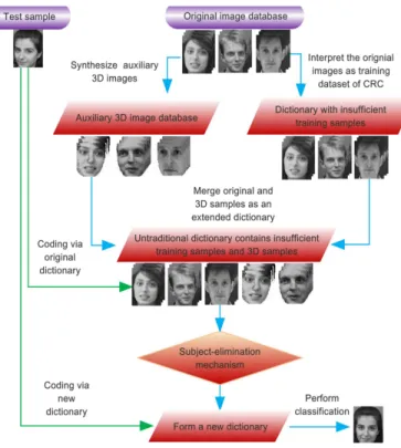
Fig. 1. The schematic diagram of the proposed framework
In facial landmark detection, random perturbations are usually applied to initial landmarks to augment the volume of a training dataset for successful landmark detector training [32]– [34]. As another concept, symmetrical faces have been used for data augmentation in face detection and classification in [35]– [37]. Xu et al. proposed to use symmetrical faces in face recognition with a sparse-representation-based method [38], [39].
Although the methods mentioned above lead to higher accuracy in face recognition or better performance in other computer vision and pattern recognition tasks, the generated virtual samples cannot tackle the problem of pose variations very well. The major drawback of traditional virtual sample generation methods is the inability to represent intra-class pose variations adequately. To be more specific, if the intra-class pose variations of test samples are different from those of the subjects in the gallery set, the information conveyed by the original training samples may not be sufficient to reconstruct them. Even an extended dictionary consisting of both original and virtual samples often lacks the capacity to represent a test face image of arbitrary pose. The traditional virtual sample generation methods used to construct an auxiliary dictionary for the relevant types of variations typically ignore the pose differences between gallery and query sets. Lastly, a large number of generated virtual samples may lead to information redundancy of the extended dictionary and data uncertainty in decision making.
To address the above issues, in this paper, we develop a method to extend an existing dictionary using a generative 3DMM. As compared to 2D generative models such as active appearance models (AAM) [32], [40], a 3DMM is capable of generating diverse face instances with arbitrary pose and illumination variations. It has been already widely used in
some computer vision applications. For example, Feng et al. used a 3DMM to generate a set of virtual faces for a facial landmark detector training and obtained state-of-the-art detection results for faces in the wild, using a cascaded collaborative regression method [41], [42]. R¨atsch et al. gener-ated virtual faces using 3DMM for 2D pose estimation using support vector regression [43]. In this paper, we propose to apply 3DMM to the training images of a given dictionary and synthesise a number of new faces with different pose variations as an auxiliary dictionary. The extended dictionary obtained using 3DMM generated entries is much better in representing different modes of variations than the original training faces alone. Moreover, a hypothesis elimination scheme with the associated on-line dictionary pruning is jointly used with the CRC method to perform face classification. Fig. 1 shows the schematic diagram of the proposed framework. The contribu-tions of our work are three-fold.
• To obtain an extended dictionary, for each 2D training example, we use a 3DMM fitting algorithm to reconstruct the 3D shape and texture information and render addi-tional face images with pose and potentially illumination variations. The original and rendered virtual faces are used to form the extended dictionary.
• To optimise the extended dictionary and address the problem of information redundancy during testing, we exploit an on-line hypothesis elimination scheme to dis-card all the training samples of the classes with inferior representation capabilities.
• We propose a CRC-based method to perform pose-invariant face classification, by mining the most represen-tative classes from the dictionary extended using 3DMM generated faces. In the rest of this paper, we use the term ‘3D Pose Dictionary integration in CRC’ (3DPD-CRC) for the proposed algorithm.
The rest of this paper is organised as follows: Section 2 overviews the relevant classical classification algorithms including SRC and CRC. They are the prerequisites to our method proposed in Section 3. Section 4 presents a theoretical analysis to the proposed method and Section 5 reports the results of comprehensive experiments conducted on the well-known ORL, FERET, PIE, GT, FRGC and LFW face datasets. Lastly, we summarise the paper in Section 6.
II. BACKGROUND
Given a dictionary with K × M training samples
{x1,1, ...,xK,M}, whereKis the number of classes andM is
the number of training samples from each class, a test sample
y∈RP can be approximated by the linear combination of all
these training samples:
y≈ K X k=1 M X m=1 αk,mxk,m, (1)
whereαk,mis the entry of the coefficient vector corresponding
to the mth training sample in thekth classxk,m∈RP, P is
the dimensionality of a sample. The entryαk,m indicates the
potential of the corresponding training sample to represent the test sample y. It should be noted that the number of training
samples of each class can be varied. Here we just use the same number, M, for convenience. In addition, Eq. (1) can compactly be rewritten as:
y≈Xα, (2) where X = [x1,1, ...,xK,M] ∈ RP×KM is the
dictio-nary matrix containing all the training samples and α =
[α1,1, ..., αKM]T is the coefficient vector need to be estimated.
Once the coefficient vector is obtained, we can measure the propensity of the kth class to represent the test sample:
ck= M X
m=1
αk,mxk,m, (3)
where ck is the reconstruction of the test sample using the
training samples merely from the kth class. The test sample reconstruction error for the kth class is obtained by:
E(y)k =ky−ck k2, (4)
and the label of the test sample yis determined using:
Label(y) = argmin
k
{E(y)k}. (5)
As stated above, the key to the classification problem is to obtain the coefficient vector reconstructing the test sample. To solve this problem, in the rest of this section, we briefly overview two algorithms: the sparse-representation-based clas-sification (SRC) [1] and collaborative-representation-based classification (CRC) [6].
1) SRC: The aim of SRC is to obtain a sparse coefficient vector αby minimising the objective function:
minkαk0 (6) s.t. y=Xα.
However, this `0-norm constrained optimisation problem is
NP-hard and difficult to solve. To address this issue, some recent studies [1], [44]–[46] demonstrate that if α is sparse enough, the solution to the above problem is equal to the solution of:
minkαk1 (7) s.t. y=Xα.
This optimisation problem can be solved by standard linear programming methods in polynomial time [47].
2) CRC: In contrast with SRC, CRC finds the coefficient vector by solving the `2-norm minimisation problem:
minkαk2 (8) s.t. y=Xα.
The optimisation of Eq. (8) is a typical least-square problem andα can be obtained by:
α= (XTX+µI)−1XTy, (9) whereµis a small positive constant andIis the identity matrix regularising the solution. It has been shown that in certain conditions the `2-norm based CRC offers competitive face
classification accuracy as compared to the`1-norm constrained
SRC, and has much lower computational complexity [6]. We propose a method that creates these conditions to enhance the performance of the CRC based face recognition.
Input 2D Image
3DMM
Fitting 3D shape and texture -15° +15° -30° +30° Synthetic Images Re nd er in g
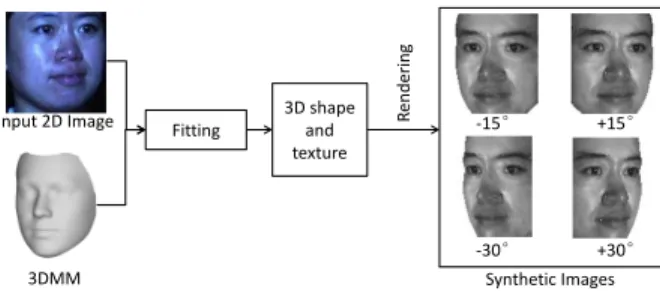
Fig. 2. Some rendered 2D faces from an input 2D image using 3DMM
III. THE PROPOSED METHOD
As discussed in Section I, the problem of existing virtual-sample-generation algorithms is that they build on the intrinsic properties of a dataset, and are unable to cater for all possible appearance variations of a subject,i.e.they are unable to inject new properties into an existing dictionary. The problem of variations in appearance can only be mitigated using an over-complete dictionary that contains training samples covering the full spectrum of appearance variations. This motivates the search for better methods to capture full gamut of appearance variations by synthesising a set of virtual trainings samples using a 3D morphable face model for CRC-based face classi-fication.
A. Synthesising virtual samples with 3DMM
A 3DMM is ideal for generating training samples with pose and illumination variations, and its use for this purpose is the tenet of our proposed method. The 3DMM approach can reconstruct the 3D shape and texture of a 2D face image by fitting a generative 3D face model to the image. To initialise the fitting process of our 3DMM, an automatic cascaded-regression-based facial landmark detection method is used [34]. Then the reconstructed 3D shape and texture are used to render 2D face images with different poses by adjusting the parameters of a camera model. For details of the 3DMM fitting algorithms the reader is referred to [26], [27], [48] and [42], respectively.
We render 2D virtual faces by projecting the reconstructed 3D shape and texture into a 2D image plane, using a perspec-tive camera. More specifically, a vertexv= [x3d, y3d, z3d]T ∈ R3 of a 3D shape is projected to a 2D coordinate s =
[x2d, y2d]T via a camera projection. The projection can be decomposed into two parts: a rigid 3D transformation Tr : R3→R3 and a perspective projection Tp:R3→R2:
Tr:v0=Rv+τ, (10) Tp:s= ox+f v0x v0 z oy−f v0y v0 z , (11)
whereR ∈R3×3 is the rotation matrix, τ ∈R3 is a spatial
translation, f denotes the focal length, and [ox, oy]T is the
optical axis of the camera in the image plane. Therefore, by setting different camera parameters {R,τ, f}, images of different poses can be rendered from the reconstructed 3D shape and texture. Some 2D face images rendered from an input face image using 3DMM are shown in Fig 2.
B. Exploiting representative classes from the extended dictio-nary
To perform dictionary integration, we use the original and synthesised virtual faces to form an extended dictionary. How-ever, this extended training dataset consisting of virtual faces with different poses is redundant and may lead to inaccurate decision making. In addition, due to the use of `2-norm
constraint, a CRC-based method cannot guarantee the sparsity of a reconstruction coefficient vector. We therefore use the extended dictionary as an initial dictionary to be refined in the next step. To this end, we use an elimination scheme that is able to identify and remove the less representative classes with the worse capacity to represent a test sample.
More specifically, we propose an iterative elimination scheme for discarding useless samples of the classes in the extended dictionary for face classification. To this end, the contribution of each class to representing a test sample is measured in terms of reconstruction error. Then all the training samples of the class with the largest reconstruction error are eliminated from the extended dictionary. The coefficient vector of the extended dictionary and the contributions of the remaining classes are then updated. The same process is repeated until the number of classes in the dictionary drops to a predefined level.
This elimination strategy strengthens those classes that are more informative and representative in reconstructing a test sample. In fact, we use Eq. (4) to estimate the reconstruction error between a specific class and a test sample, which is a distance measurement between a test sample and the linear combination of all training samples from the class. A larger value of the reconstruction error means that the training sam-ples of the class make tiny contributions in representing a test sample, and consequently this class should be eliminated from the extended dictionary. A further analysis to the proposed method is presented in the next section. The pipeline of our 3DPD-CRC face classification algorithm is shown in Fig. 3.
IV. ANALYSIS OF THE PROPOSED METHOD
To reveal the nature of the proposed method, in this section, we further analyse our 3DPD-CRC from both theoretical and empirical perspectives.
A. Improvements and the underlying rationale
Let X˜ denote the augmented dictionary, created from the original training setXand the synthesised setXˆ. Further, let
e
αi = [αi1, ..., αiM,αˆi1, ...,αˆiV]T be the vector of CRC
co-efficients reconstructing input pattern y, using the augmented dictionaryX˜. Let us assume that ybelongs to classi.
In order to explain the need for the proposed augmentation of the training set and the on-line dictionary pruning by hypothesis elimination, we shall consider a few examples:
Case 1: Suppose the synthesised training samples are not available. Then, ideally, only the coefficients for class i
associated with the original training samples should be non-zero, i.e. α ≈[0, ...,0, αi1, ..., αiM,0, ...,0]T. However, this
assumption only holds when the test sample y is exactly the same as one of the training samples of the ith class in
1: inputA dictionary consisting of a set of training samples
X= [x1,1, ...,xK,M] and a test sampley;
2: A 3DMM is applied to all the samples in the training set to obtain their reconstructed 3D facesX3D= [x31D, ...,x3KD];
3: For each reconstructed 3D face scanx3kD, we renderV 2D virtual faces {xˆk,1, ...,ˆxk,V}. This results in an auxiliary
dataset Xˆ = [ˆx1,1, ...,ˆxK,V]that consisting of all the 2D
virtual faces rendered from their reconstructed 3D face scans.
4: An extended dictionary X˜ = [X,Xˆ] is constructed us-ing both the original 2D images and their virtual faces rendered from their reconstructed 3D face scans;
5: forl= 1 toL(a pre-defined parameter)do
6: Encode the test sample using CRC and obtain the coefficient vector, as described in Eq. (9);
7: Compute the reconstruction error of each class using Eq. (4) and eliminate all the training samples of the class achieving the largest reconstruction error to update the dictionary;
8: end for
9: return The label of the test sample using Eq. (5).
Fig. 3. The proposed 3DPD-CRC algorithm
the dictionary. In practical applications, both the samples in the dictionary X and the test sample y may contain image degradation caused by appearance variations or noises. In such a case, the coefficients of unrelated training samples will be increased and that of the samples of the ith class will be decreased. As the data set does not contain enough samples to represent different poses, theithclass fitting error ||y−Xiαi||2 will be quite high, causing misclassification.
Case 2: Suppose we have injected (by means of syn-thesised samples) dictionary items which represent sample
y very well. This will be reflected in coefficients αij
tak-ing higher values (responses) for synthesised samples and lower values (responses) for original samples. Ideally, the coefficients of the original samples would be close to zero,
i.e. αei ≈ [0, ...,0,αˆi1, ...,αˆiV]T. However, pose variation
may bring larger appearance variations than the variations in identity in terms of Euclidean distance. If at the same time we have injected redundancy that is enabling samples from other classes to contribute actively to the reconstruction of patterny, this will create an opportunity for CRC to dilute the strength of coefficientsαˆij and distribute their weight over samples from
the other classes,i.e. over coefficients αˆkj,∀k6=i. As these
samples furnish similar information, their impact is that the total weight needed for the reconstruction is divided between them. To be more specific, this will reduce the value of an element in αei and increase the values of the elements in e
αk associated with the synthesised faces that have the same
pose of y. For the same approximation error, the `2 norm
minimisation will prefer this weight-diluting solution, as the sum of many small values squared is much smaller than the sum of a few larger weights squared. The reconstruction of
y in the presence of redundancy will reduce the weights of samples from class i, increasing the approximation error, and potentially leading to misclassification.
0 5 1 0 1 5 2 0 2 5 3 0 3 5 4 0 0 . 2 0 . 3 0 . 4 0 . 5 0 . 6 0 . 7 0 . 8 0 . 9 1 . 0 1 . 1 R e s id u a l e rr o r ( a ) O r i g i n a l t r a i n i n g s e t
(a) The original dictionary
0 5 1 0 1 5 2 0 2 5 3 0 3 5 4 0 0 . 2 0 . 3 0 . 4 0 . 5 0 . 6 0 . 7 0 . 8 0 . 9 1 . 0 1 . 1 R e s id u a l e rr o r ( b ) O r i g i n a l t r a i n i n g s e t
(b) The original dictionary with the elimina-tion strategy 0 5 1 0 1 5 2 0 2 5 3 0 3 5 4 0 0 . 2 0 . 3 0 . 4 0 . 5 0 . 6 0 . 7 0 . 8 0 . 9 1 . 0 1 . 1 R e s id u a l e rr o r ( c ) E x t e n d e d t r a i n i n g s e t w i t h 3 D s a m p l e s
(c) The extended dictionary
0 5 1 0 1 5 2 0 2 5 3 0 3 5 4 0 0 . 2 0 . 3 0 . 4 0 . 5 0 . 6 0 . 7 0 . 8 0 . 9 1 . 0 1 . 1 R e s id u a l e rr o r ( d ) E x t e n d e d t r a i n i n g s e t w i t h 3 D s a m p l e s
(d) The extended dictionary with the elimina-tion strategy
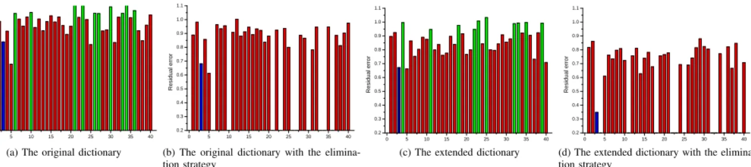
Fig. 4. Reconstruction errors of a test image using: (a) the original dictionary; (b) the original dictionary with the elimination strategy; (c) the extended dictionary consisting of virtual faces generated by 3DMM; and (d) the extended dictionary with the elimination strategy. The blue bars indicate the correct label for the test sample, and the green bars indicate the classes should be discarded from the dictionary using the proposed elimination scheme.
Case 3: If a systematic on-line elimination of the training samples from the clutter hypotheses (classes with high approx-imation error) is carried out, the redundancy is suppressed. The pruning process will increase the weight of coefficients αˆij
and enhance their ability to reconstruct the input pattern with low error, thus leading to correct identification of the class membership ofy. The hypothesis elimination process induces sparsity in a manner similar to the Iterative Hard Thresholding algorithm [49].
B. An empirical explanation of the proposed method
In this section, we present an empirical explanation of the proposed 3DPD-CRC algorithm. To demonstrate how the proposed method works, Fig. 4 shows the reconstruction error of a test sample using the training samples of each class in the dictionary, evaluated on the ORL face dataset that has 40 subjects and each subject has 10 face images. We used the first two face images per subject as training samples and the remaining 8 images as test samples. Fig. 4 shows the reconstruction errors of a randomly selected test sample from the 3rd subject. The reconstruction errors of the test sample by the correct class are highlighted using blue bars. Green bars indicate the classes with higher reconstruction errors and should be discarded during the elimination scheme.
The reconstruction errors of the selected test sample using the classical CRC algorithm by 40 classes of the original dictionary without elimination are shown in Fig. 4(a). The 3rd class does not have the minimal reconstruction error and the label of the test sample is assigned to the 5th class that pro-vides best representation to the test sample. According to the underlying assumption of the proposed elimination scheme, a larger error indicates that the corresponding class (with green bar) in the dictionary has tiny effects on representing a test sample hence should be eliminated from the dictionary. Hence, we iteratively discard some classes from the original dictionary and re-calculate the reconstruction error of the test sample by each class, as shown in Fig. 4(b). The reconstruction error of the test sample by the third class is reduced when using fewer classes in the original dictionary, but it is still higher than that of the 5th class and lead to inaccurate decision making.
To demonstrate the merit of the proposed data augmentation method, we repeated the above procedure using the extended dictionary with 3DMM synthesised virtual training faces.
The results are shown in Fig. 4(c) (without elimination) and Fig. 4(d) (with elimination). The single use of the extended dictionary also reduces the reconstruction error of the test sample by the correct class, i.e. the 3rd class, as shown in Fig. 4(c). However, the reconstruction error of the 5th class is still the minimal one thereby leading to an incorrect face classification result. But, as shown in Fig. 4(d), the reconstruction error of the test sample from the 3rd class is greatly reduced and the correct classification result can be achieved by jointly using the extended dictionary and the elimination scheme.
From this experiment, we can suggest that the joint use of virtual training samples and the elimination scheme in our 3DPD-CRC improves the accuracy of face classification. Moreover, the proposed method results in a dictionary learned from a dynamic optimisation process, which increases the sparsity of the reconstruction coefficient vectors obtained by CRC.
V. EXPERIMENTALRESULTS
In this section, we evaluate the proposed 3DPD-CRC algo-rithm on six face datasets: ORL [50], FERET [51], PIE [52], GT [53], LFW [54] and FRGC [55].
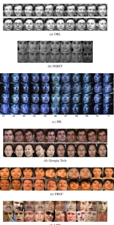
The ORL dataset contains 40 subjects and each subject has 10 face images. The images were captured at different time in-stances, with slightly varying lighting conditions, expressions, and artefacts. Some examples of ORL are shown in Fig. 5a.
The FERET dataset is a result of the FERET program, which was sponsored by the U.S. Department of Defence through the DARPA program [51]. It has become a very popu-lar benchmarking dataset for the evaluation of face recognition techniques. The proposed algorithm was evaluated on a subset of FERET, which includes 1400 images of 200 individuals with 7 different images per subject. Some examples of the FERET dataset are shown in Fig. 5b.
The CMU PIE dataset consists of 41,368 images of 68 individuals with mixed variations in pose, expression and illumination. The images of each subject were captured under 13 poses, 43 illuminations and 4 expressions. The proposed algorithm was evaluated on a subset of the PIE dataset, which includes 2992 images of 68 subjects. Each subject has all the 11 pose variations and 4 illumination variations, as shown in Fig. 5c. The selected images are with the camera id of c22,
(a) ORL (b) FERET (c) PIE (d) Georgia Tech (e) FRGC (f) LFW
Fig. 5. Example faces of the ORL, FERET, PIE, Georgia Tech, FRGC and LFW datasets
c25, c02, c37, c05, c27, c29, c11, c31, c14 and c34, which are relabelled as pose 01-11.
The Georgia Tech face database [53] was collected by the Georgia Institute of Technology. This database has the face images of 50 subjects, captured over two or three sessions. Each subject in the dataset has 15 colour images with a cluttered background. The images show frontal and/or tilted faces with expression and illumination variations. All the images were resized to 40 by 30 in our experiments. Some example images from the Georgia Tech face database are shown in Fig. 5d.
The Face Recognition Grand Challenge (FRGC) version 2 database [55] consists of controlled and uncontrolled colour face images. The controlled images present good image qual-ity, whereas the uncontrolled images of poor image quality
are taken under complex backgrounds. In this paper, we select 100 individuals with 30 different images of each subject from FRGC to construct our experimental subset. We resize each face image in this subset to 80 by 80. Some images from the FRGC database are shown in Fig. 5e.
LFW [54] is one of the most challenging unconstrained datasets and consists of face images characterised by abundant variations, including pose, illumination and expression varia-tions. The LFW database has 13,233 images of 5749 subjects. The proposed algorithm is evaluated on a subset of the LFW database, which includes 1580 images of 158 individuals with 10 different images of each subject. We resized each face image in the LFW database to 64 by 64. Some images from the LFW database are shown in Fig. 5f.
A. Results on ORL
For the ORL face dataset, we followed the evaluation protocol that has been widely used in previous studies [29], [56], [57]. We randomly selected θ(θ = 2,3,4) samples of each subject for training and the remaining ones were used for test. Thus, a training set of 40×θ images and a test set with40×(10−θ)images were created in each experiment. We repeated our experiment 10 times and measured the accuracy of different face classification algorithms in terms of recognition rate. Meanwhile, we applied 3DMM fitting to each training sample and synthesised 10 virtual faces with ±4◦, ±8◦, ±12◦, ±16◦ and ±20◦ yaw rotations. The elimination scheme presented in Section 3.2 was performed in classification.
The classification results of SRC [1], CRC [6] and the proposed 3DPD-CRC on ORL with 2, 3 and 4 training samples are presented in Table I, Table II and Table III, respectively. In these tables, the term ‘elimination proportion’ indicates the proportion of the removed classes in the elimination phase. It should be noted that the elimination strategy was used for all these three algorithms. As shown in Table I, II and III, the proposed 3DPD-CRC method using the extended hybrid dictionary outperforms the classical CRC and SRC in terms of accuracy, regardless of the proportion of the eliminated classes and the number of training samples. The results validate the effectiveness of the proposed method of jointly using synthesised virtual faces and the elimination scheme. However, it is hard to determine the best value of the elimination proportion because different methods perform best at different proportions of the eliminated classes. One practical solution to this issue is to tune this parameter using cross validation for a specific face recognition task.
Table IV presents the recognition rates achieved by a set of traditional face classification methods including SRC [1], CRC [6], LRC [58], L21SDA [59], TPTSR [56], ESRC [29], CFFR [57] and SFRC [38], as well as the proposed 3DPD-CRC method, using 2 or 3 training samples of each class in the original dictionary. The proposed 3DPD-CRC method achieves 88.0% and 92.8% recognition rates when using only 2 and 3 samples per subject as training samples. These results are better than those achieved by all the other methods.
TABLE I
FACE RECOGNITION RATES(%)OF DIFFERENT METHODS WITH2RANDOMLY SELECTED TRAINING SAMPLES ONORL
Method Elimination Proportion
10% 20% 30% 40% 50% 60% 70% 80% 90%
3DPD-CRC 85.5±0.06 86.3±0.05 86.3±0.05 86.7±0.06 87.0±0.08 87.0±0.05 87.2±0.07 87.3±0.07 88.0±0.05
SRC [1] 52.2±2.99 79.2±1.53 83.7±2.24 85.4±2.51 85.4±2.47 84.7±2.26 85.7±2.29 83.7±2.32 82.6±2.07 CRC [6] 82.8±2.48 83.4±2.37 83.9±2.16 84.5±2.62 85.4±2.65 85.9±1.93 86.2±2.12 85.6±2.49 84.1±2.47
TABLE II
FACE RECOGNITION RATES(%)OF DIFFERENT METHODS WITH3RANDOMLY SELECTED TRAINING SAMPLES ONORL
Method Elimination Proportion
10% 20% 30% 40% 50% 60% 70% 80% 90%
3DPD-CRC 91.6±0.11 91.3±0.08 92.5±0.11 92.5±0.11 93.4±0.14 93.1±0.12 93.1±0.11 92.8±0.11 92.8±0.12 SRC [1] 79.5±1.90 89.4±1.66 90.0±1.37 91.0±1.17 90.5±1.42 89.8±1.54 91.1±0.95 89.0±1.70 88.7±1.72 CRC [6] 88.1±1.79 88.3±2.08 89.0±1.76 89.1±1.59 90.3±1.64 91.2±1.21 91.3±1.35 91.6±0.89 90.6±1.60
TABLE III
FACE RECOGNITION RATES(%)OF DIFFERENT METHODS WITH4RANDOMLY SELECTED TRAINING SAMPLES ONORL
Method Elimination Proportion
10% 20% 30% 40% 50% 60% 70% 80% 90%
3DPD-CRC 96.5±0.02 96.9±0.02 97.1±0.02 97.1±0.02 96.9±0.02 96.8±0.02 96.8±0.02 96.9±0.02 97.2±0.02
SRC [1] 91.1±1.26 92.3±1.68 92.9±1.51 92.8±1.25 92.2±1.20 92.2±1.24 93.7±1.30 91.8±1.80 91.0±1.39 CRC [6] 90.1±1.60 91.0±1.87 91.4±1.89 91.9±1.52 92.0±1.51 92.5±1.26 93.0±1.05 93.8±0.94 92.7±0.93
TABLE IV
FACE RECOGNITION RATES(%)OF DIFFERENT METHODS ONORL Method Number of training samples
2 3 SRC [1] 85.7 91.1 CRC [6] 86.2 91.6 LRC [58] 84.6 90.2 SDA-L2 [59] 80.5 82.1 TPTSR [56] 83.4 87.8 ESRC [29] 87.1 89.6 CFFR [57] 83.2 88.4 SFRC [38] 87.7 91.3 3DPD-CRC 88.0 92.8 B. Results on FERET
For the FERET dataset, the same procedure as in ORL was used to split the original dataset into training and test sets. This evaluation protocol is compliant with that used in similar experiments reported in the literature. The number of training samples per subject was set to θ(θ= 2,3,4), which resulted in a training set with200×θimages and a test set with200×
(7−θ) images. To obtain the extended dictionary, we used 3DMM to fit each training sample and rendered 10 virtual samples with the same pose variations as in the last section.
The face classification results of SRC, CRC, and our 3DPD-CRC on FERET are shown in Table V, Table VI and Table VII using 2, 3 and 4 training samples per subject in the original dictionary. The elimination strategy was used for all these three methods. As shown in these tables, in conjunction with the elimination scheme, the proposed 3DPD-CRC method consistently achieves better classification results than SRC and CRC, regardless of the elimination propotion and the number of training samples.
The face classification results of SRC [1], CRC [6],
pose-01(c22) pose-09(c31)pose-10(c14) 0 0.1 0.2 0.3 0.4 0.5 0.6 0.7 0.8 0.9 1 CRC SRC LRC 3DPD-CRC
Fig. 6. A comparison of different methods in face recognition on the PIE face dataset, partitioned by different pose variations.
LRC [58], L21SDA [59], TPTSR [56], ESRC [29], CFFR [57], SFRC [38], PCA+LDA [60] and our 3DPD-CRC on the FERET dataset are presented in Table VIII. The table presents the face recognition rates of different algorithms using both 2 and 3 randomly selected training samples per class in the original dictionary. We repeated our experiment 10 times and report the average recognition rate. According to this table, the proposed 3DPD-CRC method achieves much better results than other methods in terms of recognition rate.
C. Results on PIE
To verify the robustness of the proposed method in pose variations, we design a specific experiment to perform sensi-tivity analysis across different pose variations. To this end, the
TABLE V
FACE RECOGNITION RATES(%)OF DIFFERENT METHODS WITH2RANDOMLY SELECTED TRAINING SAMPLES ONFERET
Method Elimination Proportion
10% 20% 30% 40% 50% 60% 70% 80% 90%
3DPD-CRC 77.7±0.36 79.4±0.34 80.6±0.29 81.1±0.25 81.1±0.26 81.5±0.17 81.4±0.15 81.3±0.16 81.0±0.19
SRC [1] 48.6±12.27 49.5±12.14 50.1±11.88 50.7±11.77 51.7±11.87 52.5±11.74 53.3±11.32 54.1±11.15 55.4±10.67 CRC [6] 45.7±10.08 46.6±10.27 47.9±9.95 48.9±10.03 50.6±9.69 52.2±10.08 54.0±10.0 55.1±10.14 55.6±9.96
TABLE VI
FACE RECOGNITION RATES(%)OF DIFFERENT METHODS WITH3RANDOMLY SELECTED TRAINING SAMPLES ONFERET
Method Elimination Proportion
10% 20% 30% 40% 50% 60% 70% 80% 90%
3DPD-CRC 93.0±0.34 93.6±0.26 94.0±0.24 93.5±0.25 93.5±0.26 93.4±0.19 93.4±0.22 93.0±0.22 92.6±0.19
SRC [1] 65.7±10.33 65.7±10.08 65.8±10.31 66.2±10.21 66.5±10.44 67.0±10.38 67.2±10.22 67.5±10.32 68.0±10.28 CRC [6] 58.7±9.82 59.6±9.99 60.6±10.18 61.7±10.31 62.7±9.91 64.3±10.56 65.6±10.14 67.8±10.08 68.7±9.45
TABLE VII
FACE RECOGNITION RATES(%)OF DIFFERENT METHODS WITH4RANDOMLY SELECTED TRAINING SAMPLES ONFERET
Method Elimination Proportion
10% 20% 30% 40% 50% 60% 70% 80% 90%
3DPD-CRC 96.5±0.29 96.9±0.25 97.1±0.25 97.1±0.27 96.9±0.19 96.8±0.20 96.8±0.19 96.9±0.17 96.5±0.20
SRC [1] 72.0±13.49 72.1±13.51 72.3±13.35 72.2±13.42 73.1±13.91 73.8±13.74 74.1±13.48 74.4±13.38 74.8±12.45 CRC [6] 62.2±12.68 62.9±12.73 64.5±13.13 65.7±13.90 67.5±13.50 68.9±13.65 70.3±13.43 72.5±13.10 74.5±11.93
TABLE VIII
FACE RECOGNITION RATES(%)OF DIFFERENT METHODS ONFERET Method Number of training samples
2 3 SRC [1] 55.4 68.0 CRC [6] 55.6 68.7 LRC [58] 66.0 74.0 TPTSR [56] 59.9 68.7 ESRC [29] 58.7 69.5 CFFR [57] 56.4 66.8 SFRC [38] 67.9 74.2 PCA+LDA [60] 52.5 62.6 3DPD-CRC 81.5 94.0
PIE face dataset was used. Specifically, the proposed algorithm and three classical representation-based classification methods, i.e.CRC, SRC and LRC, were evaluated on a subset of the PIE dataset. The subset has 2992 images of 68 individuals with 11 pose variations, including0◦ (pose 06),±22.5◦(pose 05, 07),
±45◦ (pose 04, 08),±67.5◦ (pose 02, 03, 09, 10) and ±90◦ (pose 01, 11) in yaw rotations, and 4 illumination variations per subject, as shown in Fig.5c. In the experiment, four frontal images (pose 06) of each subject were used to create the gallery dictionary and all the remaining images were used for test. In the proposed 3DPD-CRC approach, we rendered 18 virtual face images for each example in the dictionary to perform dictionary augmentation. The virtual face images were synthesised from ±10◦ to ±90◦ in yaw with the interval of 10◦.
The results of SRC, CRC, LRC and our 3DPD-CRC are shown in Fig. 6. According to this figure, the proposed 3DPD-CRC method performs much better than SRC, 3DPD-CRC and LRC in terms of face classification accuracy across all different head rotations. It should be noted that the improvements achieved by the proposed method on PIE are much higher than that on the other datasets. The main reason is that this PIE subset
TABLE IX
FACE RECOGNITION RATES(%)OF DIFFERENT METHODS ONGT Method Number of training samples
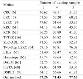
3 4 5 CRC [6] 46.62 48.51 51.75 LRC [58] 53.53 57.20 60.22 ESRC [29] 47.67 51.64 53.85 RRC [61] 44.13 43.44 45.70 RCR [62] 36.25 37.89 41.20 TPTSR [56] 58.50 65.82 75.82 SLC-ADL [63] 41.53 49.09 52.83 Two-Step LSRC [64] 59.16 67.81 76.08 L1LS [65] 51.40 52.47 61.66 Homotopy [66] 45.74 49.64 52.46 DALM [67] 52.75 57.61 61.30 FISTA [68] 48.93 51.99 53.05 DSRL2 [69] 54.12 56.66 61.82 Our method 67.26 71.45 77.63
contains much more variations in appearance than the others. In such scenarios, the superiority of our algorithm is more dramatic.
D. Results on GT database
As in the previous experiments, we repeat our experi-ments 10 times and report the average recognition rate as the final result. In each round of the experiment on the GT database, θ (θ = 3, 4, 5) per subject were randomly chosen for training, and the remaining images were used for testing. A comparison of the recognition rates of the various methods, including CRC [6], LRC [58], ESRC [29], RRC [61], RCR [62], TPTSR [56], SLC-ADL [63], Two-Step LSRC [64], L1LS [65], Homotopy [66], DALM [67], FISTA [68] and DSRL2 [69], is presented in Table IX.
From the experimental results reported in Table IX, we can see that our method achieves the best recognition rates of 67.26
TABLE X
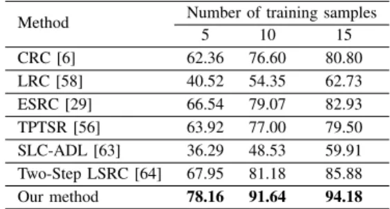
FACE RECOGNITION RATES(%)OF DIFFERENT METHODS ONFRGC Method Number of training samples
5 10 15 CRC [6] 62.36 76.60 80.80 LRC [58] 40.52 54.35 62.73 ESRC [29] 66.54 79.07 82.93 TPTSR [56] 63.92 77.00 79.50 SLC-ADL [63] 36.29 48.53 59.91 Two-Step LSRC [64] 67.95 81.18 85.88 Our method 78.16 91.64 94.18
%, 71.45%, and 77.63%withθ(θ= 3,4,5)training samples. The proposed approach outperforms all the other typical sparse (or collaborative) representation-based classification methods.
E. Results on FRGC database
For the FRGC database, θ(θ= 5,10,15) training samples of each class were selected to construct the training set and the remaining ones were used for test. The face classification results of CRC [6], LRC [58], ESRC [29], TPTSR [56], SLC-ADL [63], Two-Step LSRC [64] and our method are presented in Table X. We repeated our experiment 10 times and report the average recognition rate. As shown in Table X, the proposed method achieves 78.16%, 91.64% and 94.18% recognition rates across different sizes of training samples, which are all better than those achieved by the other methods. This is attributed to the fact that the collaborative representa-tion is performed based on the augmented dicrepresenta-tionary and the proposed elimination scheme.
F. Results on LFW database
In each round of the experiment on the LFW database, we randomly selected θ(θ = 1,2,3,4) training samples per subject for training, and the remaining samples were used for test. We measured the accuracy of different face classification algorithms in terms of recognition rate. The recognition rate of the proposed method is compared to CRC [6], LRC [58], ESRC [29], TPTSR [56], SLC-ADL [63] and Two-Step LSRC [64]. We repeated our experiment 10 times and report the average recognition rate.
As shown in Table XI, the proposed method performs much better than the other methods in terms of face classification accuracy across all different sizes of training sets. It should be noted that the improvements achieved by the proposed method on the PIE and LFW datasets are much higher than those on the ORL, FERET, GT and FRGC datasets. This is mainly because the LFW and PIE datasets contain more variations in appearance than the other datasets. In such scenarios, the superiority of our algorithm is more evident compared to other sparse (or collaborative) representation-based methods.
In light of the experimental results achieved by the different datasets mentioned above, we can conclude that the proposed method achieves more effective and stable performance in terms of recognition rate, regardless of the number of training samples per subject.
TABLE XI
FACE RECOGNITION RATES(%)OF DIFFERENT METHODS ONLFW Method Number of training samples
1 2 3 4 CRC [6] 8.34 11.58 14.03 15.63 LRC [58] 4.67 7.87 10.89 13.01 ESRC [29] 9.06 14.16 17.23 19.97 TPTSR [56] 10.09 17.79 19.59 23.81 SLC-ADL [63] 3.86 7.69 10.84 13.82 Two-Step LSRC [64] 11.17 18.35 21.42 25.40 Our method 20.02 33.75 43.81 51.96 G. Experiment on different datasets using VGG-CNN-based features
In recent years, deep neural networks have been successfully used for a variety of pattern recognition and computer vision tasks and have become the main streams in the areas. A deep network has strong capability in extracting robust image features supporting accurate classification of images with appearance variations. With such robust image features, even a very simple classifier, e.g. the nearest neighbour classifier, can work well. The proposed approach does not aim at beating deep neural networks for robust feature extraction. In fact, the proposed approach should be treated as a more powerful classifier that can be jointly used with deep neural networks. Note that, all the experiments reported in the last few sub-sections were conducted on raw image intensities. To validate the effectiveness of the proposed approach when using deep-neural-networks-based image features, we compare the proposed method with Support Vector Machine (SVM) for the task of face classification, using VGG-CNN features. To be more specific, we use the pre-trained VGG face model [70] to extract CNN features, rather than the use of original image intensity features. The 4096-D vector output from the second fully connected layer of VGG is used as the features of an input face image. To use VGG in the proposed 3DPD-CRC method, the VGG face model is applied to the test image and all the images in the augmented dictionary with both original and synthesised faces. This step was conducted between Step 3 and Step 4 in the classical 3DPD-CRC algorithm (Fig. 3). For SVM, we directly applied the VGG face model to all the training and test images to extract CNN-based facial features. Then the extracted VGG-CNN features were used for face classification with the SVM classifier.
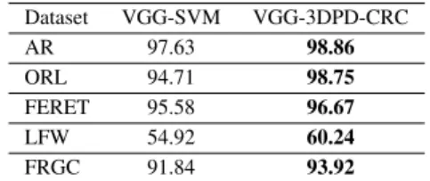
We have conducted experiments on the AR, ORL, FERET, LFW and FRGC datasets. For each subject of different dataset, a single image is randomly selected for training and the remaining images are used for test. We repeated our exper-iment 10 times and measured the performance of different face classification algorithms in terms of recognition rate. The face recognition rates are reported in Table XII. The proposed method consistently outperforms the SVM classifier on all the datasets in terms of face recognition accuracy, when using robust deep-learning-based facial features. This further validates the effectiveness of the proposed classification approach.
TABLE XII
EXPERIMENT ON DIFFERENT DATASETS USINGVGG-CNN-BASED FEATURES. Dataset VGG-SVM VGG-3DPD-CRC AR 97.63 98.86 ORL 94.71 98.75 FERET 95.58 96.67 LFW 54.92 60.24 FRGC 91.84 93.92 VI. CONCLUSION
In this paper, we proposed a dictionary integration algorithm using 3D morphable face models for pose-invariant CRC-based face classification. The key innovation of the proposed method is to accomplish face recognition by utilizing 3DMM for training data augmentation, which makes CRC robust to pose variations. The strength of the technique lies in successfully generating virtual faces with pose variations using 3DMM, and thereby enhancing the capacity of the dictionary to reconstruct input signals faithfully. Moreover, the extended dictionary is optimised on-line using an elimination scheme, which further improves the accuracy of the proposed face classification algorithm. We believe that our promising results will encourage more work on synthesising an informative dictionary and lead to successful solutions for other application domains in the future.
REFERENCES
[1] J. Wright, A. Y. Yang, A. Ganesh, S. S. Sastry, and Y. Ma, “Robust face recognition via sparse representation,”IEEE Transactions on Pattern Analysis and Machine Intelligence, vol. 31, no. 2, pp. 210–227, 2009. [2] E. G. Ortiz, A. Wright, and M. Shah, “Face recognition in movie trailers
via mean sequence sparse representation-based classification,” inIEEE International Conference on Computer Vision., 2013.
[3] D. Chen, X. Cao, F. Wen, and J. Sun, “Blessing of dimensionality: High-dimensional feature and its efficient compression for face verification,” inIEEE International Conference on Computer Vision, 2013. [4] M. Yang, L. Zhang, J. Yang, and D. Zhang, “Metaface learning for sparse
representation based face recognition,” inIEEE International Conference on Image Processing, 2010.
[5] C.-G. Li, J. Guo, and H.-G. Zhang, “Local sparse representation based classification,” in International Conference on Pattern Recognition, 2010.
[6] L. Zhang, M. Yang, X. Feng, Y. Ma, and D. Zhang, “Collaborative representation based classification for face recognition,”arXiv preprint arXiv:1204.2358, 2012.
[7] D. Zhang, M. Yang, and X. Feng, “Sparse representation or collabo-rative representation: Which helps face recognition?” inInternational Conference on Computer Vision, 2011.
[8] X. Song, Z.-H. Feng, G. Hu, X. Yang, J. Yang, and Y. Qi, “Progressive sparse representation-based classification using local discrete cosine transform evaluation for image recognition,” Journal of Electronic Imaging, vol. 24, no. 5, pp. 053 010–053 010, 2015.
[9] X. Song, Z.-H. Feng, X. Yang, X. Wu, and J. Yang, “Towards multi-scale fuzzy sparse discriminant analysis using local third-order tensor model of face images,”Neurocomputing, vol. 185, pp. 53–63, 2016. [10] H. S. Lee and D. Kim, “Tensor-based aam with continuous
varia-tion estimavaria-tion: applicavaria-tion to variavaria-tion-robust face recognivaria-tion.”IEEE Transactions on Pattern Analysis and Machine Intelligence, vol. 31, no. 6, pp. 1102–16, 2009.
[11] S. Yan, D. Xu, Q. Yang, L. Zhang, X. Tang, and H. J. Zhang, “Multi-linear discriminant analysis for face recognition,”IEEE Transactions on Image Processing, vol. 16, no. 1, pp. 212–20, 2007.
[12] S. T. Roweis and L. K. Saul, “Nonlinear dimensionality reduction by locally linear embedding,”Science, vol. 290, no. 5500, p. 2323, 2000. [13] M. Belkin and P. Niyogi, “Laplacian eigenmaps for dimensionality
reduction and data representation,”Neural Computation, vol. 15, no. 6, pp. 1373–1396, 2006.
[14] X. He and P. Niyogi, “Locality preserving projections,” Advances in Neural Information Processing Systems, vol. 16, no. 1, pp. 186–197, 2003.
[15] S. Z. Li, L. Zhu, Z. Zhang, A. Blake, H. Zhang, and H. Shum, “Statistical learning of multi-view face detection,” in European Conference on Computer Vision, 2002, pp. 67–81.
[16] Z.-H. Feng, J. Kittler, M. Awais, P. Huber, and X.-J. Wu, “Face detection, bounding box aggregation and pose estimation for robust facial landmark localisation in the wild,” inThe IEEE Conference on Computer Vision and Pattern Recognition Workshops (CVPRW), 2017, pp. 160–169. [17] Z.-H. Feng, J. Kittler, W. Christmas, P. Huber, and X.-J. Wu, “Dynamic
attention-controlled cascaded shape regression exploiting training data augmentation and fuzzy-set sample weighting,” inThe IEEE Conference on Computer Vision and Pattern Recognition, 2017, pp. 2481–2490. [18] V. Blanz and T. Vetter, “Face recognition based on fitting a 3D
morphable model,”IEEE Transactions on Pattern Analysis and Machine Intelligence, vol. 25, no. 9, pp. 1063–1074, 2003.
[19] X. Chai, S. Shan, X. Chen, and W. Gao, “Locally linear regression for pose-invariant face recognition,”IEEE Transactions on Image Process-ing, vol. 16, no. 7, pp. 1716–1725, 2007.
[20] P. Koppen, Z.-H. Feng, J. Kittler, M. Awais, W. Christmas, X.-J. Wu, and H.-F. Yin, “Gaussian mixture 3d morphable face model,” Pattern Recognition, vol. 74, pp. 617–628, 2018.
[21] Z. Zhu, P. Luo, X. Wang, and X. Tang, “Deep learning identity-preserving face space,” inIEEE International Conference on Computer Vision, 2013, pp. 113–120.
[22] ——, “Multi-view perceptron: a deep model for learning face identity and view representations,” inInternational Conference on Neural Infor-mation Processing Systems, 2014, pp. 217–225.
[23] J. Yim, H. Jung, B. I. Yoo, C. Choi, D. Park, and J. Kim, “Rotating your face using multi-task deep neural network,” inIEEE Conference on Computer Vision and Pattern Recognition, 2015, pp. 676–684. [24] G. Hu, F. Yan, C. H. Chan, W. Deng, W. Christmas, J. Kittler, and N. M.
Robertson, “Face recognition using a unified 3d morphable model,” in
European Conference on Computer Vision, 2016, pp. 73–89.
[25] W. Deng, J. Hu, Z. Wu, and J. Guo, “Lighting-aware face frontalization for unconstrained face recognition,” Pattern Recognition, vol. 68, pp. 260–271, 2017.
[26] J. T. Rodriguez, “3D Face Modelling for 2D+3D Face Recognition,” Ph.D. dissertation, Surrey University, Guildford, UK, 2007.
[27] G. Hu, P. Mortazavian, J. Kittler, and W. Christmas, “A facial symmetry prior for improved illumination fitting of 3D morphable model,” in2013 International Conference on Biometrics, 2013, pp. 1–6.
[28] T. Vetter, “Synthesis of novel views from a single face image,”IJCV, vol. 28, no. 2, pp. 103–116, 1998.
[29] W. Deng, J. Hu, and J. Guo, “Extended SRC: Undersampled face recognition via intraclass variant dictionary,” IEEE Transactions on Pattern Analysis and Machine Intelligence, vol. 34, no. 9, pp. 1864– 1870, 2012.
[30] Y.-S. Ryu and S.-Y. Oh, “Simple hybrid classifier for face recognition with adaptively generated virtual data,” Pattern recognition letters, vol. 23, no. 7, pp. 833–841, 2002.
[31] D. Beymer and T. Poggio, “Face recognition from one example view,” inInternational Conference on Computer Vision, 1995.
[32] T. F. Cootes, G. J. Edwards, C. J. Tayloret al., “Active appearance mod-els,”IEEE Transactions on pattern analysis and machine intelligence, vol. 23, no. 6, pp. 681–685, 2001.
[33] X. Cao, Y. Wei, F. Wen, and J. Sun, “Face alignment by explicit shape regression,”International Journal of Computer Vision, vol. 107, no. 2, pp. 177–190, 2014.
[34] Z.-H. Feng, P. Huber, J. Kittler, W. Christmas, and X.-J. Wu, “Random cascaded-regression copse for robust facial landmark detection,”IEEE Signal Processing Letters, vol. 1, no. 22, pp. 76–80, 2015.
[35] M.-C. Su and C.-H. Chou, “Application of associative memory in human face detection,” inIJCNN, 1999.
[36] S. Saha and S. Bandyopadhyay, “A symmetry based face detection technique,” inWieNSET, 2007.
[37] E. Saber and A. M. Tekalp, “Frontal-view face detection and facial fea-ture extraction using color, shape and symmetry based cost functions,”
Pattern Recognition Letters, vol. 19, no. 8, pp. 669–680, 1998. [38] Y. Xu, X. Zhu, Z. Li, G. Liu, Y. Lu, and H. Liu, “Using the original
and ‘symmetrical face’training samples to perform representation based two-step face recognition,”Pattern Recognition, vol. 46, no. 4, pp. 1151– 1158, 2013.
[39] Y. Xu, X. Li, J. Yang, Z. Lai, and D. Zhang, “Integrating conventional and inverse representation for face recognition,”IEEE Trans. on Cyber-netics, vol. 44, no. 10, pp. 1738–1746, 2014.
[40] Z.-H. Feng, J. Kittler, W. Christmas, X.-J. Wu, and S. Pfeiffer, “Auto-matic face annotation by multilinear aam with missing values,” in21st International Conference on Pattern Recognition (ICPR). IEEE, 2012, pp. 2586–2589.
[41] Z.-H. Feng, G. Hu, J. Kittler, W. Christmas, and X.-J. Wu, “Cascaded collaborative regression for robust facial landmark detection trained using a mixture of synthetic and real images with dynamic weighting,”
IEEE Transactions on Image Processing, vol. 24, no. 11, pp. 3425–3440, 2015.
[42] J. Kittler, P. Huber, Z.-H. Feng, G. Hu, and W. Christmas, “3D Morphable Face Models and Their Applications,” in9th International Conference on Articulated Motion and Deformable Objects, vol. 9756, 2016, pp. 185–206.
[43] M. R¨atsch, P. Huber, P. Quick, T. Frank, and T. Vetter, “Wavelet Reduced Support Vector Regression for Efficient and Robust Head Pose Estimation,” inIEEE Ninth Conference on Computer and Robot Vision, 2012, pp. 260–267.
[44] D. L. Donoho, “For most large underdetermined systems of linear equations the minimal`1-norm solution is also the sparsest solution,”
Communications on pure and applied mathematics, vol. 59, no. 6, pp. 797–829, 2006.
[45] E. J. Candes, J. K. Romberg, and T. Tao, “Stable signal recovery from incomplete and inaccurate measurements,”Communications on pure and applied mathematics, vol. 59, no. 8, pp. 1207–1223, 2006.
[46] E. J. Candes and T. Tao, “Near-optimal signal recovery from random projections: Universal encoding strategies?”IEEE Trans. on Information Theory, vol. 52, no. 12, pp. 5406–5425, 2006.
[47] S. S. Chen, D. L. Donoho, and M. A. Saunders, “Atomic decomposition by basis pursuit,”SIAM journal on scientific computing, vol. 20, no. 1, pp. 33–61, 1998.
[48] P. Huber, Z.-H. Feng, W. Christmas, J. Kittler, and M. R¨atsch, “Fitting 3d morphable face models using local features,” inIEEE International Conference on Image Processing, 2015, pp. 1195–1199.
[49] T. Blumensath and M. E. Davies, “Iterative hard thresholding for compressed sensing,”Applied and Computational Harmonic Analysis, vol. 27, no. 3, pp. 265–274, 2009.
[50] T. Heap and F. Samaria, “Real-time hand tracking and gesture recogni-tion using smart snakes,”Proc. Interface to Human and Virtual Worlds, Montpellier, France, p. 50, 1995.
[51] P. J. Phillips, H. Moon, S. A. Rizvi, and P. J. Rauss, “The FERET evaluation methodology for face-recognition algorithms,”IEEE Trans-actions on Pattern Analysis and Machine Intelligence, vol. 22, no. 10, pp. 1090–1104, 2000.
[52] T. Sim, S. Baker, and M. Bsat, “The CMU pose, illumination, and ex-pression database,”IEEE Transactions on Pattern Analysis and Machine Intelligence, vol. 25, no. 12, pp. 1615–1618, 2003.
[53] A. Nefian, “Georgia tech face database,” 2013.
[54] M. M. B. T. Huang, G. B and E. Learned-Miller, “Labeled faces in the wild: A database for studying face recognition in unconstrained environments,” inMonth, 2008.
[55] P. J. Phillips, P. J. Flynn, T. Scruggs, K. W. Bowyer, J. Chang, K. Hoffman, J. Marques, J. Min, and W. Worek, “Overview of the face recognition grand challenge,” inIEEE Conference on Computer Vision and Pattern Recognition, 2005, pp. 947–954.
[56] Y. Xu, D. Zhang, J. Yang, and J.-Y. Yang, “A two-phase test sample sparse representation method for use with face recognition,” IEEE Transactions on Circuits and Systems for Video Technology, vol. 21, no. 9, pp. 1255–1262, 2011.
[57] Y. Xu, Q. Zhu, Z. Fan, D. Zhang, J. Mi, and Z. Lai, “Using the idea of the sparse representation to perform coarse-to-fine face recognition,”
Information Sciences, vol. 238, pp. 138–148, 2013.
[58] I. Naseem, R. Togneri, and M. Bennamoun, “Linear regression for face recognition,”IEEE Transactions on Pattern Analysis and Machine Intelligence, vol. 32, no. 11, pp. 2106–2112, 2010.
[59] X. Shi, Y. Yang, Z. Guo, and Z. Lai, “Face recognition by sparse discriminant analysis via joint L 2, 1-norm minimization,” Pattern Recognition, vol. 47, no. 7, pp. 2447–2453, 2014.
[60] J. Yang and J.-y. Yang, “Why can LDA be performed in PCA trans-formed space?”Pattern recognition, vol. 36, no. 2, pp. 563–566, 2003. [61] M. Yang, L. Zhang, J. Yang, and D. Zhang, “Regularized robust coding for face recognition,”IEEE Transactions on Image Processing, vol. 22, no. 5, pp. 1753–1766, 2013.
[62] M. Yang, L. Zhang, D. Zhang, and S. Wang, “Relaxed collaborative rep-resentation for pattern classification,” inIEEE Conference on Computer Vision and Pattern Recognition, 2012, pp. 2224–2231.
[63] J. Wang, Y. Guo, J. Guo, M. Li, and X. Kong, “Synthesis linear classifier based analysis dictionary learning for pattern classification,”
Neurocomputing, vol. 238, pp. 103–113, 2017.
[64] C. Shao, X. Song, Z. H. Feng, X. J. Wu, and Y. Zheng, “Dynamic dictionary optimization for sparse-representation-based face classifica-tion using local difference images,”Information Sciences, vol. 393, pp. 1–14, 2017.
[65] K. Koh, S. Kim, S. Boyd, and Y. Lin, “l1 ls: A simple matlab solver for`1-regularized least squares problems,”URL: http://www. stanford.
edu/˜ boyd/l1 ls/(Last viewed 11/4/2008), 2007.
[66] A. Y. Yang, S. S. Sastry, A. Ganesh, and Y. Ma, “Fast 1-minimization algorithms and an application in robust face recognition: A review,” in
IEEE International Conference on Image Processing, 2010.
[67] A. Y. Yang, Z. Zhou, A. G. Balasubramanian, S. S. Sastry, and Y. Ma, “Fast `1-minimization algorithms for robust face recognition,” IEEE Transactions on Image Processing, vol. 22, no. 8, pp. 3234–3246, 2013. [68] A. Beck and M. Teboulle, “A fast iterative shrinkage-thresholding algo-rithm for linear inverse problems,”Siam Journal on Imaging Sciences, vol. 2, no. 1, pp. 183–202, 2009.
[69] Y. Xu, Z. Zhong, J. Yang, J. You, and D. Zhang, “A new discriminative sparse representation method for robust face recognition via l{2}
regularization,” IEEE transactions on neural networks and learning systems, vol. 28, no. 10, pp. 2233–2242, 2017.
[70] O. M. Parkhi, A. Vedaldi, and A. Zisserman, “Deep face recognition,” inBritish Machine Vision Conference, 2015.
Xiaoning Songreceived the B.S. degree in computer science from Southeast University, Nanjing, China, in 1997, the M.S. degree in Computer Science from Jiangsu University of Science and Technology, Zhenjiang, China, in 2005, and the Ph.D. degree in pattern recognition and intelligence system from the Nanjing University of Science and Technology, Nan-jing, in 2010. He was a Visiting Researcher with the Centre for Vision, Speech, and Signal Processing, University of Surrey, Guildford, U.K., from 2014 to 2015. He is currently an Associate Professor with the School of Internet of Things Engineering, Jiangnan University, Wuxi, China. His current research interests include pattern recognition, machine learning and computer vision.
Zhen-Hua Feng (S’13-M’16) received the Ph.D. degree from the Centre for Vision, Speech and Signal Processing, University of Surrey, Guildford, U.K. in 2016. He is currently a research fellow at the University of Surrey. His research interests include pattern recognition, machine learning and computer vision. He has publications in major conferences and journals including CVPR, TIP, PR, etc. He has received the European Biometrics Industry Award 2017 from the European Association for Biometrics.
Guosheng Hu (S’13-M’16) is a senior scientist in AnyVision. Prior to that, he worked as a research fellow in THOTH group, INRIA. He received the PhD degree from the University of Surrey, UK, in 2015. His research interests include pattern recogni-tion, biometrics, machine learning and graphics.
Josef Kittler (M’74-LM’12) received the B.A., Ph.D., and D.Sc. degrees from the University of Cambridge, in 1971, 1974, and 1991, respectively. He is Professor of Machine Intelligence at the Centre for Vision, Speech and Signal Processing, University of Surrey, Guildford, U.K. He conducts research in biometrics, video and image database retrieval, medical image analysis, and cognitive vision. He published the textbook Pattern Recognition: A Sta-tistical Approach and over 600 scientific papers. He serves on the Editorial Board of several scientific journals in pattern recognition and computer vision.
Xiao-Jun Wureceived the B.Sc. degree in math-ematics from Nanjing Normal University, Nanjing, China, in 1991. He received the M.S. degree and the Ph.D. degree in pattern recognition and intelligent systems from Nanjing University of Science and Technology, Nanjing, China, in 1996 and 2002, respectively. He is currently a Professor in artificial intelligent and pattern recognition at Jiangnan Uni-versity, Wuxi, China. His current research interests include pattern recognition, computer vision, fuzzy systems, neural networks, and intelligent systems.