Implied Calibration of Stochastic Volatility Jump Diffusion
Models
S. Galluccio
∗, Y. Le Cam
‡∗
BNPParibas, London,
‡Université d’Evry Val d’Essonne
First version: July 2005
This version: September 2005
Abstract
In the context of arbitrage-free modelling of financial derivatives, we introduce a novel cal-ibration technique for models in the affine-quadratic class for the purpose of contingent claims pricing and risk-management. In particular, we aim at calibrating a stochastic volatility jump diffusion model to the whole market volatility surface at any given time. We numerically im-plement the algorithm and show that the proposed approach is both stable and accurate.
∗Corresponding author: Stefano Galluccio, BNP Paribas Fixed Income, 10 Harewood Avenue, London NW1 6AA, United Kingdom. stefano.galluccio@bnpparibas.com.
Keywords: Linear-Quadratic models, Option pricing, Model calibration
JEL classification: G12, G13.
Acknowledgments: We are grateful to M. Jeanblanc, M. Yandle, O.Scaillet, and to the participants at the 2005 Financial Modelling Workshop at the Newton Institute (Cambridge), the 2005 ICBI Global Derivatives Conference (Paris), the 2005 Risk-Management Conference (Rome) and the 2005 Derivatives RISK Conference (London) for helpful comments.
1
Introduction
A number of studies have demonstrated that the simple Black-Scholes (BS) paradigm of lognormality of asset returns distribution is in contrast with empirical observations. The simplistic assumption of asset dynamics being driven by a Gaussian process must indeed be rejected in favour of more general processes like, for instance, those driving stochastic volatility (SV) models.
One stream of research focuses on the statistical properties of asset returns. In this context, empirical evidence seems to reject SV models since they are not capable of reproducing the observed conditional kurtosis of returns. The presence of jumps is often advocated as a solution to this problem. In fact, evidence of presence of jumps in the asset, in the volatility or in both is reported in Bates (1996), Bakshi et al. (1997), Chernov et al. (1999), Andersen et al.(2002), Pan (2002), Bates (2000), Erakeret al. (2003) and Chernovet al. (2003), among others.
In another set of studies, departures from the BS model are advocated in relation to the implied volatility smile phenomenon. Deterministic volatility extensions of the BS model were first due to Dupire (1994) and Derman and Kani (1994). These are usually referred to as local volatility (LV) models. Although LV models provide a simple mechanism for smile generation, they are pledged by a number of shortcomings. On the empirical side, they require the knowledge of option prices over a continuum of strikes and maturities, a situation never encountered in practice. On the theoretical side, it is well-known (Rebonato (2000), Andersen and Andreasen (2000)) that models whose volatility evolves deterministically with the underlying state variables generate smiles at future times that are inconsistent with historical observations: while historical smile surfaces display a high degree of time-stationarity, model-implied smiles in LV models tend to flatten very quickly as time goes by. In addition, by imposing a deterministic relationship between volatility and underlying, one is implicitly making a strong assumption on their relative movements, with implications on the risk-management side (Di Graziano and Galluccio (2005)). Empirical literature rejects local volatility models on their impact on hedging, Dumas et al. (1997). In a different line of thought, Hull and White (1987), Stein and Stein (1991) and Heston (1993), account for the smile phenomenon through SV models. Finally, modelling the smile through mixed jump-diffusion (JD) processes is proposed in Andersen et al. (2000) (for LV models with jumps) and Duffie et al. (2000) (for SV models with jumps). However, to force a SV or a JD model to be consistent with the whole set of smiles at different maturities (the so-called “implied volatility surface”), model coefficients must be heavily (and unrealistically) time-dependent. In particular, SV models tend to underestimate smile convexity at short maturities while a JD model suffers from the same drawback at large maturities (Section 3).
reject SV, JD and LV models in favour of stochastic volatility jump-diffusion models (SVJD) thanks to their superior market explicative power.
A fundamental problem in the applications (e.g. for derivatives pricing and hedging) is the esti-mation of latent parameters in SVJD models. Estiesti-mation based on statistical analysis from historical data series has been given extensive coverage in the past. In particular Bates (2000), Chernov et al. (1999), Craine, Lochstoer and Syrtveit (2000) and Deelstra et al. (2002) use simulation-based estimators and/or Efficient Methods of Moments in models with jumps and stochastic volatility. Erakeret al. (2003) employ Markov Chain Monte Carlo methods to provide evidence of jumps in both asset and volatility. Finally, extensive empirical studies across several models are conducted in Chernovet al. (2003).
As long as option pricing and hedging is concerned, a model must be made consistent with the available market quotations of liquid vanilla options in order to avoid arbitrage opportunities. In this respect statistical estimations must be replaced or, at least, complemented by a reverse engineering process (model calibration) that consists of determining model parameters to reproduce the observed vanilla option prices1. Despite the importance of having a fast, robust and accurate
model calibration, the literature on the subject is scarce. In this respect, calibration based on short-term asymptotics is studied in Medvedev and Scaillet (2004). Backuset al. (1997) and Zhang and Xiang (2005) use an interesting mapping to infer a term structure of market implied cumulants directly from market smiles at different maturities. Unfortunately, this approach does not provide an estimation of the coefficients of a single model that is consistent with the whole volatility surface since different models are needed to match different smiles. Bakshiet al. (1997) and Andersen and Andreasen (2000) suggest to calibrate a model by minimizing the sum of the squared errors of all available options across all strikes and maturities. This simple non-linear least squares optimization is usually not convergent and not statistically robust, as shown in Cont and Tankov (2004) and Detlefsen (2005). Cont and Tankov point out that the information contained in the set of available option prices is not sufficient to remove the coefficients degeneracy that is associated to a SVJD process and suggest that calibration can only be achieved provided one adds exogenous information in addition to the available option prices. For, they introduce a calibration algorithm (in the context of exponential-Lévy processes) where the objective function contains a convex functional that is meant to stabilize the (non-convex) optimization problem. The authors are mainly interested in calibrating a single smile at the time, but a straight generalization of Cont-Tankov’s approach to more general processes or to cope with the calibration of the whole volatility surface remains, as of
1When market is complete, model calibration identifies (at least in principle) the unique risk-neutral measure and avoids the problem of determining the market price of risk. This contrasts the case when estimation is conducted from a statistical perspective. When market is incomplete, calibration allows selecting the “market” measure among the infinite set of possible risk-neutral measures.
today, an open issue.
In our paper, inspired by Cont and Tankov (2004) results, we attempt to take the next step in this direction and introduce a novel implied calibration methodology for some SVJD models with time-dependent coefficients in the affine-quadratic class (Piazzesi (2003), Peng and Scaillet (2004)). We recall that the affine-quadratic class contains the affine one as a special case. Our approach, aimed at calibrating the whole volatility surface at any given time, retains (at a qualitative level) some of the interesting features contained in Cont and Tankov’s method, namely the regularization of least-squares optimization through addition of a number of constraints to the problem. However, we depart from Cont and Tankov method in both the nature of the problem (we aim at calibrating the whole volatility surface as opposed to a single smile curve) and in the type of dynamics (we don’t restrict ourselves to Lévy processes). We apply our method to one of the simplest (yet non-trivial) SVJD model with jumps in the asset and we show that an accurate and financially meaningful calibration to the whole volatility surface is possible and the algorithm is robust. However, our study strongly suggests that the algorithmic complexity is such that generalizing the present approach to more complex models might result impossible to achieve. This is the case, for instance, when jumps in volatility are also present or for more general local volatility forms .2 These shortcomings expose
an intrinsic limitation of SVJD models and clearly indicate that, despite their mathematical and financial appeal, further theoretical developments are needed.
The rest of the paper is organized as follows. In section 2 we introduce model and notations, and we determine closed-form formulae for European options. In Section 3 we analyze the different role played by jumps and stochastic volatility in explaining the market smile. This results in identifying two separate regimes which are instrumental in solving the calibration problem. Section 4 gathers some general ideas about calibration in models mixing jumps and stochastic volatility while Section 5 is devoted to a detailed description of the calibration methodology. Numerical results are presented in Section 6 and Section 7 contains conclusions and prospects for future research.
2
Mathematical setup and option pricing
2.1
The model
Let(Ω,A,P) be a probability space. We shall denote bySt the price of the Equity asset at time
t and rt the spot rate of interest assumed deterministic. A probability measure P∗, equivalent to the historical probability measure P, is said to be the risk-neutral measure if the relative price
Ste−rttfollows a local martingale process underP∗.
2One important exception being hybrid (Equity-IR) modelling with no jumps in volatility since in that case the approach we present here can be applied without major modifications, as shown in Galluccio and LeCam (2005).
We stipulate that the asset dynamics follows a jump-diffusion process under any equivalent risk-neutral measureP∗,3 dSt St− = (rt−dt−µt)dt+ηtdB 1 t +dJt dηt=λ(at−ηt)dt+αtdB2t, (1)
where B1 and B2 are two Brownian motions with dB1, B2
t = ρ1,2(t)dt; λ is a constant and
dt, αt, atare deterministic functions of time. Here,J is a compound Poisson process with stochastic intensityξ(t, St). We shall writeJt=n≥1
eYn
−11{Tn≤t} (Ti are the jump arrival times), and denote byGthe law of the jumps (aiidsequence). More precisely, the jump diffusionZ = (S, η)is a Feller process with infinitesimal generatorAdefined by
Aϕ(t, x) = ∂tϕ+∂xϕ(t, x)ζ(t, x) + 1 2tr ∂x,xϕ(t, x)Σ(t, x)Σ(t, x) (2) +ξ(t, x) R [ϕ(t, x1+u)−ϕ(t, x)]dG(u),
whereζ is the drift vector andΣthe volatility matrix of the diffusion. Letµt=ξ(t, St)E∗(Y)be its associated compensator. An equivalent representation considers state variables driven by a two dimensional vector of independent Wiener processesW1, W2
dS t St− = (r−dt−µt)dt+ηtdW 1 t +dJt dηt=λ(at−ηt)dt+αtρ1dWt1+ρ2dWt2 (3)
where{ρi:=ρi(t), i= 1,2}are deterministic functions of time. We will alternate between the first and the second representation depending on the circumstances, if no confusion arises. The relation between the two representations is provided byρ1=ρ1,2, ρ2
1+ρ22= 1.
As it is well known, the above model is arbitrage-free but is not complete. Model calibration will then be used to select the risk-neutral measure. We also remind that the model defined by Eqs. (1) and(3)does not belong to the affine class, in the sense of Duffieet al. (2000), since it corresponds the jumps-augmented version of the Stein-Stein model, (Stein and Stein (1991)). The equivalent of(1) within the affine framework (when (Yn)n≥1 are Gaussian r.v.’s) is in fact the Bates (1996) model which is obtained by assuming thatη2
t follows a one-dimensional CIR-like process.
Our choice is motivated by a number of reasons. First, empirical literature (Jones (2003), Aït-Sahalia and Kimmel (2004)) demonstrates that simple affine models must be rejected in favor of more general processes. Indeed, our model belongs to the so called “linear-quadratic” class (Piazzesi (2003), Peng and Scaillet (2004)), which includes the affine as a special case. Second, our calibration
3For sake of simplicity, we will thoroughout assume that the divident processdtis deterministic and that relative dividends are payed continuously in time. Note also that in our formulation no restriction must be imposed on the r.v. Y to ensure thatStstays positive.
algorithm (Sections 4 and 5) applies without major changes to affine models as well. Finally, SVJD linear-quadratic models can be easily generalized to include quanto and cross-currency features as well as the effect of stochastic interest rates (for the purpose of hybrids modelling) while this is not possible in affine models (Galluccio and Le Cam (2005)). At an intuitive level, the presence of quanto effects or stochastic interest rates induces non-linear terms in the drift of the process. As a consequence, apart from rather unrealistic situations (for instance when some correlations are artificially set to zero so to force these non-linear additional terms to identically vanish, see Galluccio and Le Cam (2005)) the CCY or stochastic interest rates extended SVJD models are not affine.
In the applications, it is useful to recast all equations in a more convenient form by introducing the auxiliary vector diffusion processXt :=
X1
t = ln (St), Xt2=ηt
and the jump process Nt :=
n≥1Yn1{Tn≤t}.In the new setting, the system reads as: dX1 t = r−1 2 X2 t 2 −dt−µt dt+X2 tdWt1+dNt dX2 t =λ at−Xt2 dt+αt ρ1dW1 t +ρ2dWt2 . (4)
The model can be efficiently handled mathematically. In fact, if we assume that the intensity process takes the form ξ(t, x) := ξ0t+ ξ1tX1
t+ ξ2tXt2+ξ3t
X2
t 2
, the jump diffusion vector-valued process
dXt=ς(Xt, t)dt+ Σ(t, Xt)dWt+dNt is a semimartingale associated to a triplet of characteristics that are affine-quadratic functions of the state variables, as in Peng and Scaillet (2004).
The presence of jumps in the dynamics is well supported by historical time series analysis, as mentioned in the introduction. Also, Bates (1996) and (2000) suggests that jumps are needed in addition to stochastic volatility to allow matching both long and short-maturity smiles within a single model. Strong evidence in support of this claim (and its implications on calibration) are given in the next Section.
2.2
Option Pricing
To ensure market consistency in pricing and hedging, a model must be “calibrated” to a set of vanilla options. The availability of closed or quasi-closed form formulae for simple European derivatives is of crucial importance to improve speed and avoid numerical convergence problems. This can be easily achieved in our framework. The path we follow is similar to the one adopted in Peng and Scaillet (2004) in the general context of affine-quadratic models.
We introduce two objects. One is the Green functionψ(u, Xt;t, T)from the risk-neutral expec-tation ψ(u, Xt;t, T) :=E∗ exp − T t R(s, Xs)ds eu·XT Gt , (5)
where R(t, Xt) = r is the spot interest rate which, for simplicity, is assumed constant. The other is the Laplace transform of the law ofY fromLf(x) = euxdG(u), under the usual conditions of existence and convergence. Next define the functionsΦi
t(x) = ξit(Lf(x)−1). Then, the following result holds (where time dependency has been omitted to lighten notation)
Proposition 1 There exist four functionsγ(t, T), β1(t, T), β2(t, T),andδ(t, T)such that ψ can be represented as ψ(u, Xt;t, T) =eγ(t,T)+β(t,T)·Xt+δ(t,T)(X 2 t) 2 foru= (u1, u2),β(t, T) := (β1(t, T), β2(t, T)), and Xt:=
Xt(1), Xt(2). Moreover the four func-tions satisfy the following system of ODE’s:
∂β1 ∂t = −Φ1(β1), ∂β2 ∂t = −Φ2(β1)−2λaδ− ρ1αβ1+ 2α2δβ 2, ∂δ ∂t = −Φ4(β1) +12 β1−β21+ 2 (λ−αρ1β1)δ−2α2δ2 ∂γ ∂t = −Φ0(β1) + (d+µ−r)β1−λaβ2−α2 δ+1 2β 2 2 (6)
with final conditionsβ(T, T) =u, δ(T, T) =γ(T, T) = 0
Proof. See Appendix A.
To allow analytical tractability of the ODE’s, avoid model overparametrization and to simplify the calibration without compromising the quality of the result we will assume, from now on, that the stochastic intensity of the compound Poisson process takes a simple form, i.e. ξ(0)t = 0, ξ(1)t =ξ(2)t =
ξ(3)t = 0. Despite this simplification, the above system contains non-linear second order Riccati equations and cannot be solved in closed form, in general. However, since only a finite set of options at different times to expiry are quoted in the market, we consider a particular specification of the ODE’s coefficients. Be(T1,· · ·, TN)the set of expiry times associated to the quoted vanilla options. Accordingly, if θ(t) is a generic time-dependent coefficient in the ODE’s system, we will assume that θ(t) is defined through piecewise constant functions as follows: θ(t) = θi, if t ∈ [Ti−1, Ti),
i = 2,· · ·, N. With this specification, on every interval [Ti−1, Ti), Riccati equations are defined in terms of constant coefficients and then solvable. On every subinterval, terminal conditions are
β(Ti) = (u1i, u2i), δ(Ti) = u3i, γ(Ti) =u4i. We then arrive at the following result, where we have definedΨi(t, x) =x−1
1−expx(Ti−t)
Proposition 2 Assume that αt, at, kt, ξt are piecewise constant on the intervals [Ti−1, Ti), i = 2,· · ·, N and that ξ(0)t = 0, ξ(1)t = ξ(2)t =ξ(3)t = 0. Then the solution of the system of ODE’s is
given, on each[Ti−1, Ti), by β(t) = u1i, M(t)u2i −K(t), δ(t) = 1 α2 i −(Bi+ Γi)− 2ΓiCi e4Γi(Ti−t) −Ci , γ(t) = u4i −d+ Φ0t(1)u1i −Φ0t(u1i)(Ti−t)−(Bi+ Γi)(Ti−t), −12ln1−Cie− 4Γi(Ti−t) 1−Ci + T t λai+1 2α 2 iβ2(s) β2(s)ds, where pi = −2λai, Ai =u1i(1−u1i)/4, Bi = αρ1u1i −λ/2, Γi2=Bi2+α2iAi, Ci= α2ui 4+Bi+ Γi α2ui 4+Bi−Γii M(t) = 1−Ci 1−Cie−4Γi(Ti−t)e −πi(Ti−t); π i= 2(Bi+ Γi)−u1ρ1αi; K(t) = 1 1−Ci −piyiΨi(t, πi) + (piyiCi−pizi) Ψi(t, πi−4Γi) zi = −2ΓiCi/α2i; yi=−Bi+ Γi/α2i.
Proof. See Appendix B.
We remark that jumps now appear in the expression of γ(t) through the Laplace transform
Lf(u1i). With a proper choice of the distribution of the r.v. Y, the transform can be analytically computed. This applies, for instance, when Y ∼ N(q, v2) is a Gaussian variable so thatL
f(x) = expqx+x2v2/2. This choice provides a simple and intuitive jumps parametrization and, as we
show below, it offers great flexibility in the calibration process.4
Our goal is the evaluation of a vanilla call option expiring at T and struck at K written onS, whose arbitrage price at time t is Callt(St, K, t, T) = E∗
exp−tTR(s, Xs)ds (ST −K)+|Gt . To this aim, we use the knowledge of the Green function
G(y, ς, ϕ, Xt;t, T) =E∗ exp − T t R(s, Xs)ds eς·XT χ(ϕ·XT≤y)|Gt , (7)
and a number of well-known results on Fourier transforms for option pricing. In fact, as the following Proposition shows,G(y, ς, ϕ, Xt, t, T) can be determined from the knowledge of ψ(u, Xt;t, T)and the pricing problem is then solved.
4In theory, a simpler solution would be to assume thatY follows a symmetric Laplace distribution with probability densityp(x) =ζexp (−ζ|x|), defined by a single parameterζ. This choice, however, does not provide enough flexibility to match the observed smiles.
Proposition 3 The price of the call option is given byCallt(St, K, t, T) =G1−KG2, with G1 = G(−lnK, ζ1, ν1, Xt, t, T), (8) withζ1 = (1,0,0), ν1= (−1,0,0), Xt= (lnSt, ηt, rt) G2 = G(−lnK, ζ2, ν2, Xt, t, T), withζ1 = (0,0,0), ν1= (−1,0,0), Xt= (lnSt, ηt, rt) and G(y, ς, ϕ, Xt, t, T) = 1 2ψ(ς, Xt, t, T)− 1 π (Rd)+ 1 kIm e−ikyψ(ς+ikϕ, X t, t, T) dk (9)
Proof. Duffie et al. (2000).
3
Gamma and Vega regimes
In this section we study the relationship between the dynamics Eq.(1) and the associated shape of the volatility surface. The goal is to provide evidence about the different role played by jumps and by stochastic volatility in explaining the observed smile in different portions of the time to expiry dimension. This result is instrumental in understanding the calibration methodology that will be introduced in Section 4.
The analysis of the moments of the asset distribution and their link with the shape of the smile has been already addressed in the literature. In particular, Backuset al. (1997) and (in a similar context) Zhang and Xiang (2005) show that if the smile is parametrized through a quadratic polynomial in the “modified moneyness”m= Σln(F/K)
atm√T−t+ Σatm
2 , whereF is the option’s underlying,Σatm is the
at the money (ATM) BS volatility andKis the strike then, approximately, the BS implied volatility at varyingmreads as σ(m, τ)Σatm√τ 1−ζ1(τ) 3! m− ζ2(τ) 4! 1−m2 , (10)
whereζ1(t)andζ2(t)are the skewness and the kurtosis of the logarithm of the underlying process, and τ = T−t is the time to expiry. This results from a Edgeworth expansion of the law of the log-asset price and holds for small values ofΣatm. Formula(10)shows the tight link existing between shape of the smile and moments of the underlying asset process. In particular, when skewness and kurtosis are zero, the smile is flat atΣatm(as in the BS model). In addition, skewness (through the linear term inm) and kurtosis (through the quadratic term in m) act by respectively tilting and bending the smile.
For the sake of simplicity, we will assume in this section that dividends dt vanish and that all model coefficients are constant since all conclusions are preserved (at a qualitative level) in the general
setup. Even in this simplified scenario the mathematical expression of the characteristic function Φt(x) :=EteixlnSTof the log-asset price (anda fortiori, that of the associated cumulants) is quite involved. For this reason, we provide explicit formulae in the pure jump case and analyze the general case numerically. When only jumps are present, Eq.(1)reduces to the Merton jump-diffusion model and the characteristic functionΦMer
t (x)reads as
ΦMert (θ) = exp (tϕ(θ)) with ϕ(θ) = ir−η2/2−µθ−η2θ2/2 +ξexpiθq
−θ2v2/2−1. In Appendix C we re-derive
this formula and show that the first four cumulants ofZt:= ln(St)are given by
E(Zt) = Π1= r−η22 t, (12) E(Zt−E(Zt))2 = Π2=V ar(Zt) =η2t+ξtq2+v2, E(Zt−E(Zt))3 = Π3=ξtqq2+ 3v2, E(Zt−E(Zt))4−3V ar(Zt)2 = Π4=ξtq4+ 6q2v2+ 3v4.
By recalling the expression of the skewnessζ1(t) = Π3Π2−3/2 and the kurtosis ζ2(t) = Π4Π−22, we
finally arrive at ζ1(t) = √1 t ξqq2+ 3v2 [η2+ξ(q2+v2)]3/2, ζ2(t) = 1 t ξq4+ 6q2v2+ 3v4 [η2+ξ(q2+v2)]2 . (13)
These equations, in conjunction with Eq.(10),show that the impact of jumps on the volatility smile is restricted at very short times. In particular the jumps-induced smile convexity decays linearly with the time to expiry while smile skewness decays ast−1/2. In a similar context to ours, Backus et al.
(1997) demonstrate that, on the opposite, the impact of stochastic volatility persists on long-term smiles.
In order to provide quantitative support to this claim and to the different roles played by jumps and stochastic volatility, in Fig.1a we show the term structure of ”butterfly spread” prices observed in the market on a generic trading day. A butterfly spread option with expiryT is a combined position in three call options and is usually measured byH= ΣBS(Katm−∆)−2ΣBS(Katm)+ΣBS(Katm+∆) where ΣBS(K) is the BS implied volatility at K. Butterfly spreads provide the simplest trading strategy to take a position in the smile’s convexity. This is due to the fact that (apart from a multiplicative factor)H is the second derivative of the smile (thought of as a function ofK) taken at Katm. Thus, the higher H the larger the convexity and viceversa. In Fig.1a we compare the market butterfly with the one generated by our model Eq.(1)in the particular case where no jumps
are present and when all coefficients are time-homogeneous.5 We see that at intermediate and at long
maturities a stochastic volatility model explains the term structure of the smile convexity reasonably well (if mean reversion is carefully chosen) but it fails to do so at short maturities. This fact has a simple and intuitive explanation. Eq.(10)shows that the smile convexity is typically associated to the excess kurtosis of the log-asset returns distribution. Since in our case this is entirely generated by a diffusion process (the volatilityηt), it normally takes time to accumulate enough kurtosis starting from 0 at inception. This implies that a simple diffusive dynamics is not consistent with the market implied smile at short maturities. These observations suggest that jumps and stochastic volatility must be combined together since jumps have a big impact on short term convexity (Eq. (13)) and stochastic volatility on long term one.
These findings can be also interpreted from a different perspective. From a trading point of view, short-term and long-term smiles have a very different origin. Short term convexity is mainly associated to investors risk aversion to unexpected economic and sociopolitical events that might result in sudden jumps in the asset price. On the other side, long-term convexity is usually driven by the law of offer/demand induced by large investors, institutions and hedge/pension funds buying and selling in and out of the money options as a form of leveraged investment. Traders refer to these two regimes as “Gamma” and “Vega” trading, since the option Gamma (resp. Vega) risk is predominant at short (resp. long) maturities and in presence of large (resp. small) asset variations. These considerations indicate that the market smile is implicitly pricing the risk of large fluctuations (indeed, jumps) in the asset dynamics in the short term and of that of unpredictable (indeed, stochastic) asset volatility in the long end. The threshold between the two regimes will be denoted byT∗.This regime “switching” is therefore an intrinsic market characteristic and plays a
fundamental role in our calibration approach.
4
SVJD models: the calibration problem
As above mentioned, model calibration consists of solving a multi-dimensional reverse engineering problem. As discussed by many authors it is impossible, in general, to determine a set of parameters such that market prices are exactly reproduced by any model.6 Throughout this paper, by “model
calibration” we then mean a methodology such that
1. The difference between market and model option prices is within the bid/ask spread.
2. The calibrated solution is statistically robust.
5In this case we recover the Stein and Stein (1991) model.
6Even from a pure financial point of view this is impossible to achieve. In fact, market imperfections and ineffi-ciencies do not allow to identify option prices exactly (a bid/ask spread is always present).
Following Cont and Tankov (2004), ideally one would attempt to perform a model calibration by solving the following general non-linear optimization problem (NS =n. of strikes, NE=n. of option expires): {ςi}∗= arg min {πi} NS j=1 NE k=1 wjk ΣTk, Kj(k);{πi} −ΣBSTk, Kj(k) 2 +ψF({πi}), (14) where {πi} is a set of free model parameters, Σ is the model-implied Black-Scholes volatility, ΣBS is the market-implied Black-Scholes volatility,ψand w
jk are weighting constants,Kj(k) is the
j-th. strike for options expiring atTk andF({πi})is a convex regularization functional. The above minimization problem provides in theory a set of “optimal” free parameters{πi}∗.
Formally, the methodology we introduce here shares some features in common with that proposal. In our case, however, because of the nature of our problem and because we aim at making the calibrated solution meaningful from a trading perspective, we add a number of additional constraints driven by statistical and risk-management criteria.
First, (condition C1) the influence of the jumps in the dynamics is confined at short times while stochastic volatility mainly acts at medium and long expiries to reflect the transition between “Gamma” and “Vega” regimes, as previously discussed. In this way we enforce smile to be generated by jumps for short maturities and by stochastic volatility for long maturities, allowing for a perfect disentanglement between the two noise sources. This assumption is crucial in the calibration process we address here but it is also beneficial in numerical implementations of PDE’s for option pricing, as extensively discussed in Galluccio and LeCam (2005). Second, (condition C2) we favour solutions where the transition between the two regimes is smooth once the model has been calibrated to liquid instruments in order to guarantee a robust risk-management. In particular, jumps will be gradually “switched off” to avoid unreasonable discontinuities in across the two regimes. Third, (condition C2) we enforce solutions where the term structure of the calibrated coefficients is as time-homogeneous as possible. From a statistical point of view, such models are more robust and realistic than those models where all parameters are heavily time-dependent. In addition, when parameters are constant the dynamics of the volatility surface is closer to stationarity and then consistent with empirical observations. This is also beneficial on the risk-management side (Rebonato (2000)).
4.1
Constrained optimization
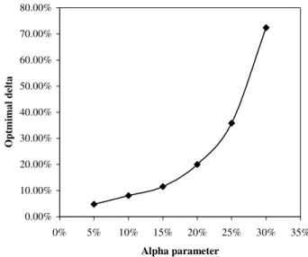
In our empirical study we consider options up to 5 years time to expiry since the market is rather illiquid at longer maturities.7 In our empirical tests we consider data from the EuroStoxx 50 equity
index, whose ATM volatility matrix is given in Fig 1b. 8 Similar studies conducted on other indeces
(S&P 500, FTSE 100, DAX and CAC40) provide similar results to the ones presented here and are available upon request. Two well-known features can be noticed. First, smile convexity is a decreasing function of time to maturity and is extremely high for short maturities. Second, the smile shape is not symmetric around the at-the-money (ATM) strike. In other words, the smile is both convex and “skewed”.
In any time interval[Ti−1, Ti)between two consecutive option expires our model is specified by a set of 7 independent constant coefficients: the volatility mean reversion levela(t), the volatility of volatility (volvol)α(t), the constant volatility mean reversion rate λη, the asset-volatility corre-lationρ1,2(t), the stochastic jumps intensity ξ(0)(t), the jumps average q(t) and, finally, the jumps variancev2(t), with t∈ [Ti−1, Ti). Obviously, any attempt to perform a global calibration on this 7-dimensional manifold is doomed to failure.9 Understanding the impact of each single parameter
on the shape of the smile is instrumental to the problem’s solution. To simplify our discussion in the beginning we will not consider the presence of jumps.
In a pure stochastic volatility framework, the role of coefficients a(t), α(t) and ρ(t) is indeed well established (Hagan et al. (2002)). For reader’s convenience, we briefly summarize the main points here. At the leading order in the volvolα(t), the at-the-money (ATM) volatility is completely specified bya(t). Thus,a(t)mainly affects the global level of the smile but has little impact on its overall shape. The Equity-IR correlationρ(t)affects the asymmetry of the smile (or “skew”) around the ATM point. Increasing correlation means that assets prices tend to increase when volatility increases and viceversa. Then, out-of-the money call and in-the-money put options become more expensive. The net effect is that implied Black volatilities at high strikes increase while Black volatilities at low strikes decrease, so that the smile takes a positively skewed shape. Similarly, the more negative the correlation, the more negatively skewed the smile. Finally, the volatility of volatility (or “volvol”) α(t)rules smile convexity: the higher α(t) the more convex the smile and viceversa. As a secondary effect, the volvol influences the total variance of the process and (just like
a(t)) it impacts the global level of the smile.10 Results displayed in Fig.2 (where the influence of 8The smooth surface has been obtained by using a BNP Paribas propietary arbitrage-free volatility interpolation algorithm that is capable of matching quoted market prices within their bid-ask spread. Alternative parametrizations have been tried, like the one proposed by Fengler (2005), but results are not significantly affected by this choice. Data correspond to Feb 2nd 2004.
9The causes for this are: i)the non-linear optimization problem is not strictly convex and,ii)some of the model parameters are quasi-degenerate. This implies that: i) the objective function has many local minima and,ii) it is almost flat in the maximum gradient direction so that both convergence and robustness are at risk (see Cont and Tankov (2004)).
10As shown in Fig. 2, by increasing the level of αthe ATM volatility increases, as one would intuitively expect. On the opposite, in affine models (Heston) the ATM volatility is inversely proportional to the volvol coefficient. This
the three parameters on the smile are compared) support this view. The picture shows that any amonga(t), α(t), ρ(t)plays a different role from the others in explaining possible smile movements. As shown below, this is a fundamental property in the calibration process.
A fundamental role is played by the mean reversionλwhich is assumed constant in our model. A mean reverting Ornstein-Uhlenbeck process converges to its ergodic measure after a “characteristic time” τ = 1/λ. The quadratic variation of the asset process in Eq.(1) is given by Qt = η2tSt2. Conditionally to any volatility path,Qtevolves like the square of a lognormal process, so it increases indefinitely on average as times goes to infinity. Becauseηis an ergodic process, its variance converges to an asymptotic value after a timet τ . Therefore, unconditionally to any realization ofηt, the average ofQtis asymptotically dominated byS2t and the effect of the stochastic volatility becomes negligible at large times. This shows that the presence of the volatility mean reversionλprovides a simple and effective tool to “fine tune” the rate of decrease of the smile convexity at long maturities, as observed in the market (see Fig. 1a, 1b). In models whereλ= 0, like the one proposed in Hagan et al. (2002), it is necessary to artificially impose a decreasing term structure of the volvol to ensure market consistency. We also remind thatλcannot be statistically inferred from historical time series since it is not measure change invariant.
When also jumps are present, the picture becomes much more complex. In fact, although jump parameters ξ(0)(t), q(t) and v(t) play altogether a role similar to a(t), α(t) andρ(t) in explaining possible smile deformations, their influence on the smile shape cannot be as nicely identified as before since, differently from above, any parameter now plays a “mixed” role. The reason for this can be best understood in the simplified scenario provided by the Merton model. In this case, the cumulants ofZt:= ln(St)are given by Eq.(12). In a BS setting we have ξ= 0, so that only mean and variance are different from zero, as expected. In this case the implied smile would be flat and equal toη. Whenξ= 0second, third and fourth cumulant play altogether a decisive role in moving the implied volatility away from its BS level. Eq. (12)and Eq. (10)show that smile deformations around the BS level can be attributed to either the stochastic intensityξ, the jumps averageqor the jumps standard deviationv. Since different triplets{ξ, q, v}can in this case be associated to almost identical smile curves the inverse problem (i.e. determining a unique triplet from a given smile or a set of smiles) is in general ill-defined (see also Cont and Tankov (2004)). When this happens we will refer to the associated parameters as being “degenerate”. This identification problem affects a number of studies, including Andersen and Andreasen (2000) and Bakshiet al. (1997). A first step towards the problem solution consists of imposing the above mentioned constraints on the problem. This goes as follows.
1. First (condition C1) we split the calibration problem in two consecutive steps. Initially, the
term structure of diffusion coefficients is kept at a (trial) constant level{a0, α0, ρ0}att < T∗,
while the smile is calibrated by only adjusting the jump coefficients as shown below. Thus, at
t < T∗, stochastic volatility does not play any role and the smile is almost entirely generated
by jumps. Once jumps calibration has been achieved, we calibrate the remaining smiles by adjusting {a(t), α(t), ρ(t)} at t ≥ T∗ while keeping the jump parameters “frozen” at their
previously calibrated levels. In this way jumps and stochastic volatility are not “mixed up” in the optimization procedure and some degeneracies (like those described in Cont and Tankov (2004) are eliminated.
2. Second, (condition C2) we impose that the switch between the two regimes at t < T∗ and t≥T∗is smooth. To meaningfully achieve this, we assume that the stochastic intensityξ(t)
is a continuous (possibly differentiable) strictly decreasing function, i.e. i) ξ(T∗) ∈ C0, ii)
ξ(T∗) = 0, iii) ξ(t)> ξ(t)fort < t. Also, the initial set{a0, α0, ρ
0}is adjusted to minimize
the jump in the value between the two regimes.
3. Third, (condition C3) the volatility mean reversionλis adjusted to ensure that the calibrated set{a(t), α(t), ρ(t)}is as time-homogeneous as possible.
5
Numerical implementation
5.1
Data set
Empirical tests on calibration are performed by using EuroStoxx 50 data on Feb, 2nd 2004. These data correspond to: a) a set of EuroStoxx forward prices for maturities up to 5Y; b) The whole EuroStoxx volatility surface for times to expiry up to 5 years. Both sets correspond to mid-market quotations and have been provided by internal BNP Paribas proprietary systems according to the market information prevailing at that time.
5.2
Jumps calibration
In the paper above mentioned, Cont and Tankov (2004) show that in Merton’s model the market-implied calibration of stochastic intensity and diffusion’s volatility from a single smile is impossible since the two parameters are degenerate. In addition, the optimization problem is not convex and many different minima exist. Although we never attempt to simultaneously calibrate jumps and
diffusion, Cont and Tankov remark equally applies if one attempts to calibrate a single smile in a Merton model.11
Unfortunately, Cont and Tankov (2004) regularization procedure for generic Lévy processes can-not be directly applied to our problem for two reasons. First, we aim at making the model consistent with the whole volatility surface and in doing so we need a term structure of model coefficients. Sec-ond, more fundamentally, the process defined by Eq. (1)is not a Lévy process since its increments are independent but not stationary.
Instead of attempting a calibration to each smile individually, we propose an alternative ap-proach aimed at calibrating the whole set of smiles up to (and including)T∗ by assuming a suitable
parametric form forξ(t)for given (constant) jumps averageqand standard deviationv.
More precisely, we aim at calibrating the three smiles corresponding to options of 1 month, 3 months and 6 months expiry, so that T∗ = 1
2 and introduce a specific form of ξ(t) according to
condition C2. We find convenient to defineξ(t) fromξ(t) = ω−ω t
δ
thanks to the fact that (as shown below) it provides excellent calibration results with a minimal number of free parameters,ω
andδ. In the applications,ξ(t)must be discretized as follows
ξ(t) =ξ(t, ω, δ) = ξ1(t, ω, δ) =ω−12ω 1 δ for t∈T0,121 ξ2(t, ω, δ) =ω−12ω 3 δ for t∈ 1 12,14 ξ3(t, ω, δ) =ω−12ω 6 δ for t∈1 4,12 , ξ(t) = 0, ift > 1 2.
With this parametrization, ξ(t) is completely specified once the two constantsω and δ have been assigned.
Initially, suppose thatδis given and that coefficients{a0, α0, ρ0}have been fixed to a trial level.
Then, the objective function
Gω,δ(q, v) := NS j=1 NE k=1 wjk ΣTk, Kj(k);q, v, ω, δ −ΣBSTk, Kj(k) 2
can be plotted as a function of(q, v)for different values of ω and the results are shown in Fig.3. Two things are worth noticing. First, the functionGω,δ(q, v)is strictly convex around a minimum independently of the chosenω (i.e. independently of the level of the jumps intensity - similar results hold at varyingδ). Second, Gω,δ(q, v)is not just locally convex around the (single) minimum but, instead, its convex portion extends to a wide region in the(q, v)space where no other local minima exist.
Table 1 provides a more rigorous argument to support this intuitive picture. There, we show the results of a simple Levenberg-Marquardt numerical minimization algorithm onGω,δ(q, v)for different
choices of the initialization set(qinit, vinit). In other words we solve the problem (q∗(ω), v∗(ω)) =
arg minq,v Gω,δ(q, v)withωgiven (in this exampleω=−0.3andδ= 1). We note that the method is very accurate for a wide range of initial conditions, although the low convexity of the surface around the minimum demands a good level of numerical accuracy. The optimization algorithm drifts away from the convex region (and provides no sensible result) only when qinit is very badly chosen at inception.
These results have been obtained by fixing the stochastic intensity to a given value. One would be tempted to try estimating the optimalω jointly with q andv, as a solution of the global least-squares problem (q∗, v∗, ω∗) = arg min
q,v,ω Gω,δ(q, v), for a given δ. This way of proceeding was suggested, for instance, in Andersen and Andreasen (2000) and Bakshiet al. (1997). Unfortunately, this direct method is not usually viable because in general{q, v, ω}is a degenerate triplet. Table 2 shows that, no matter howωis selected, it always exists an optimal couple(q∗(ω), v∗(ω))such that
the objective functionGω(q∗(ω), v∗(ω))attains the same minimum value. Thus, Gω(q∗(ω), v∗(ω)) is almost flat inω and the inverse (minimization) problem onω is ill-posed.
To overcome this potential issue, we introduce a convex penalization term, as in Cont and Tankov (2004). In the present case, however, the relative-entropy (or Kullback-Leibler distance) method used by the authors cannot be applied since ours is not a Lévy process. We then introduce a quadratic penalization term so that the whole inverse problem reads in general as
(q∗(ω), v∗(ω)) = arg min (q,v) NS j=1 NE k=1 wjk ΣTk, Kj(k);q, v, ω, δ −ΣBSTk, Kj(k) 2 , (15) (ω∗, q∗, v∗) = arg min ω (qP−q∗(ω))2+ (vP−v∗(ω))2. (16) Simply stated, the problem consists of determining ω∗ such that the couple (q∗, v∗)is as close as
possible to a “prior” couple qP, vP arbitrarily chosen. A good criterion is to estimate jumps average and standard deviation from historical data series and to assignqP, vPaccordingly. This choice has the advantage that the optimal solution(ω∗, q∗, v∗)is a guarantee that the market-implied
model stays “close” (in the probability measure space) to the historically estimated one. 12
Although the above methodology provides a unique and stable solution, the resulting errors between market and model implied smiles can sometimes be beyond the typical volatility bid/ask spread (i.e., 1% in lognormal units) if δ is badly chosen. In fact, calibration accuracy sensibly depends on the choice ofξ(t). Whenδ= 1, the simple hyperbolic shape associated toξ(t)does not
1 2As an important remark, we note that the request that couplesqP
, vP
and(q∗, v∗)are close is a well defined problem in probabilistic terms. In fact, this is equivalent to enforce that the market-implied jumps probability distri-bution is as close as possible to the historical (ob jective) one. Girsanov theorem ensures that the jumps distridistri-bution is indeed invariant under changes of probability measure (in our case from the objective to the risk-neutral and viceversa).
provide good results while precision can be improved by modifyingδ(i.e., by changing the speed of convergence ofξ(t)to 0ast→T∗).
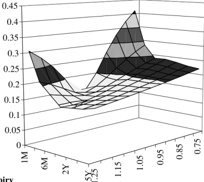
The main question is how does the choice ofδimpact the above picture and whether any complex interplay between the choice ofδ and that ofω exists destroying the above picture. To study this problem in Fig. 4a we report the results of an optimization performed on δ, i.e., for a given set
{a0, ρ0, α0, ω}we solve the problem
δ∗= arg min
δ Gω,δ(q, v), (17)
and we look at how this optimal solution is affected by changes in the trial set{a0, ρ0, α0, ω}. Let
G∗=Gω,δ∗(q, v)be the minimum of the objective function. We consider a typical set of parameters
as our base case scenario (Series 1). All other curves in Fig.4a are obtained from the base one by applying a large shock in one single parameter among those in the set{a0, ρ0, α0, ω}. Results can be
summarized as follows,i)δ∗ andG∗ are not sensibly affected by a shock inω anda0,ii) a shock in ρ0 affects calibration accuracy (G∗) but has almost no impact on the optimalδ∗,iii) a shock inα
0
affects the optimalδ∗but has almost no impact on the calibration accuracy (G∗). In addition, Fig4b
further investigates the dependency ofδ∗ onα0. The picture shows that the functional relationship
betweenδ∗andα0 is linear only for small values ofα0.
These results indicate that the choice of the optimalδ∗is almost entirely dependent on the chosen value of α0. in other words, once the initial volvol parameter has been set at inception, one can
determine an optimalδ∗ for any given set of{a0, ρ0, ω}by solving problem(17).Even though after
calibration to the smileω will be different, δ∗ is guaranteed to stay very close to the new optimal value. The conclusion is that, once the initial volvolα0assigned, jumps can be efficiently calibrated
to the market.
5.3
Stochastic volatility calibration
In the last section we showed that it is possible to calibrate the jumps once an initial set{a0, ρ0, α0}
of SV parameters has been assigned. We now address the issue of how optimally select the triplet
{a0, ρ0, α0}. In general, unfortunately, there is no unique answer to this, i.e., there is no obvious
way to decide how to fix a priori the triplet before any calibration is attempted. Despite finding a unique set is impossible, we introduce a constructive approach that allows calibrating the model efficiently. The good news is that, once this “pre-calibration” study has been carried out, the initial set{a0, ρ0, α0}can be taken as granted and one can avoid readjusting it too often (see Section 6 on
this point).
The approach we use is based on the intuitive observation that if {a0, ρ0, α0} has been badly
impossible to calibrate the remaining smiles for options expiring afterT∗. To better understand the
link between{a0, ρ0, α0}and terminal variance, skewness and kurtosis we have performed a number
of tests. As an illustration, we consider three sets of parameters a0, ρ0, α(0i)
, with i = 1,2,3 corresponding to α(1)0 = 10%, α(2)0 = 30%, α(3)0 = 50%. For each given set, the model is then calibrated to all smiles up to 6 months expiry as previously explained. Finally, all smiles with expiry beyond 6 months are generated. This test is aimed at measuring the terminal variance, skewness and kurtosis generated by the initial set {a0, ρ0, α0} (and by jumps) and to check whether they
are compatible with the market prices. Table 3 gathers the results. There, we show the difference between market and model implied volatility for smiles at 1Y, 2Y, 3Y and 5Y induced by the calibration at shorter maturities. Results show that, as one might expect, if α0 is assigned a too
high value at the beginning, model-implied smiles at 1Y expiry are inconsistent with the market. In our case, ifα0 = 50%the terminal variance at 1Y is too high: no matter how {a(t), ρ(t), α(t)}
are selected in the time interval [6M,1Y] hitting the market smile is impossible. In theory, this could still be achievable by allowinga(t)to take large negative values but this solution is financially meaningless.
We can formally define, for a givena0, a “critical” valueα0 of the volvol coefficient as follows:
α0= sup{α0:all smiles are calibrated within the bid/ask spread;a(t)>0, α(t)>0}.
In other words, α0 is the maximum value of the volvol such that, other parameters being given,
all smiles can be matched by means of a sequence{a(t), ρ(t), α(t)}by keeping botha(t)and α(t) positive. In the next section we show that calibration can be achieved for a wide range of α0 by
performing a full volatility surface calibration (i.e.,α0 is normally very high). We finally remark
that the above picture is not significantly altered by ρ0 once its sign has been properly assigned (smiles are usually negatively skewed implyingρ0should be always negative). These two properties are extremely important since they indicate that{a0, ρ0, α0}can be assigned with great flexibility
without compromising the quality of the calibration.
We now assume that{a0, ρ0, α0}has been fixed and that an optimal set{ω∗, q∗, v∗, δ∗}has been
determined accordingly. The next step consists of keeping these parameters fixed and calibrate the remaining part of the volatility surface att≥T∗by adjusting the stochastic volatility coefficients a(t), α(t)andρ(t). In other words, starting from the first smile afterT∗, we proceed recursively and
at each interval in between consecutive smiles we attempt solving the following problem
(α∗(t), ρ∗(t), a∗(t)) = arg min a(t),α(t),ρ(t) NS j=1 ujk ΣTk, Kj(k);α(t), ρ(t), a(t) −ΣBSTk, Kj(k) 2 , (18) fort ∈ [Tk, Tk+1), k= 1,· · ·, L−1, T1=T∗, (19)
whereL−1is the number of smiles with expiry strictly larger thanT∗. As above anticipated, this
problem is well posed since{α∗(t), ρ∗(t), a∗(t)}are not degenerate.
Finally,λcan be fine tuned so that the calibrated term structure of the volvola∗(t)is as constant
as possible. Finding the optimal λ∗ can be easily achieved by solving the following least squares optimization, λ∗= arg min λ L−1 j=1 α∗j(λ)−α∗j+1(λ)2 , (20) where vector (α∗
1(λ), α∗2(λ),· · ·, α∗L(λ)) comprises the piecewise constant term structure of α∗(t), for a given value of λ. In short, λ∗ is the volatility mean reversion that corresponds to the least oscillating calibrated term structure a∗(t). As before, the good news is that once optimization
problem(20)has been solved it is possible to keepλ∗fixed without significantly altering the result in future calibrations. In this way, we empirically established that optimal values forλare in the interval[0.4,0.7],independently on the chosen market.
6
Calibration algorithm and numerical results
6.1
The algorithm
In our example, we calibrate the model on a set of increasing time to expiry options, corresponding toT1= 1 month,T2=3 months, T3=6 months, T4=1 year, T5=2 years, T6=3 years, T7=5
years. T0 is the observation date. We define a thresholdT∗ between the two regimes. In our test
we fixT∗= 0.5, but similar results can generally be found by fixingT∗ anywhere between 3 months
and 1 year. We callT< the set of option expiries shorter thanT∗, that is T<:={T :T ≤T∗}, with
|T<|=M<. Similarly,T>:={T :T > T∗}, with|T>|=M>. The calibration algorithm is based on a recursive procedure that, starting from the shortest expiryT1,proceeds as follows.
1. Choose a “trial” value for λ. Then run a “pre-calibration” test as described in the previous section to determine, for a given a0, the critical volvol coefficientα0. Finally, determine an
initial set{a0, ρ0, α0}by fixingα0<α0.
2. Assign a value toω and determineδ∗ such that the calibration errors inT< are minimal by solving(17), while{a0, ρ0, α0}are kept fixed at their initial values.
3. Withδ∗ fixed, calibrate the jumps coefficients inT< by solving the two optimization problems (15)and (16). In other words, for a given ω solve (15)so thatω∗ corresponds to the single ω such that the quadratic distance betweenqH, vHand(q∗, v∗)is minimal. This procedure
4. Next, determine the diffusion coefficients by calibrating the smile in the intervalT>. Keep jump parameters frozen at the previously calibrated values, then proceed recursively by sequentially calibrating the remaining smiles starting from the one associated to options with the shortest maturity in T>. This is done by solving the problem (18) and provides an optimal term structure of SV coefficients{α∗(t), ρ∗(t), a∗(t)}fort≥T∗.
5. If the prior mean reversion rateλ(0)has been badly chosen, step 4) might provide a too rapidly increasing or decreasing term structure{α∗(t), ρ∗(t), a∗(t)}, as previously discussed. We then
proceed (condition C3) by solving the problem(20): choose a new λ(1) and restart from step 1). Then proceed recursively until the optimalλ∗ has been found.
As already discussed, it is not necessary to perform all five steps at any new calibration. For instanceδ∗andλ∗are very stable with time and, once estimated, can be occasionally readjusted. In addition, if one is not interested in ensuring that couple(q∗, v∗)is close to the historically estimated
one, step 3) can be neglected in the algorithm.
Extensive empirical studies performed on S&P and EuroStoxx data in the time period spanning the years 2002 - 2005 (not reported here) suggest that the optimalλ∗must lie in the interval[0.4,0.7],
as above mentioned. Interestingly, this is in contrast with the most recent findings of λbased on historical data series (Erakeret al. (2000)) that assign to the mean reversion rate much lower values:
λ∈[0.013,0.025]. This indirectly indicates that the market price of volatility risk is significant in SVJD models.
6.2
Numerical results
In all our tests we calibrate each smile by selecting three liquid options (i.e.,NS = 3) struck atKi,
i = 1,2,3. These correspond to the at-the-money forward option (K2), one in-the-money option
(K1), and one out of-the-money option(K3). All results are however independent fromNS.To ensure selection of liquid (and meaningful) points, for every expiryTiwe fixK1(resp. K3) to a fixed number
lof standard deviations from the ATM strike, i.e. K1=K0−lσAT M
√
T, K3 =K0+lσAT M
√ T. Here,σAT M is the at-the-money Black implied volatility13. Scale parameterlis fixed to 1, although
larger values can be considered in case one needs to calibrate wider portions of the smile. Fixingl
to a too large value must be avoided since far out of the money or in the money options are illiquid. Spot interest rate is0.033and dividends are 0. All weightsujk, wjk are fixed to 1.
Tables 4 and 5 show results of a typical calibration on the EuroStoxx volatility matrix for
α0 = 10% and α0 = 30%, while a0 = 6% is given. We see that (given two quite different values
1 3Alternatively one could selectK
1(resp. K3) as the strike corresponding to 25% (resp. 75%) of the ATM option’s
of the initial volvol coefficient) the model is capable of efficiently calibrating the whole volatility surface since all errors are within the bid ask spread (typically around 1%). However, when α0 is
set to10%, the resulting term structure ofα(t)is much more irregular than in the second case with
α0 = 30%. In particular, a jump in α(t) exists between the 6 month and the 1Y smile. When
this happens, adjusting λcan help in partially reducing the oscillations ofα(t), but to completely remove the jumps it is usually necessary to adjustα0,as Table 5 demonstrates. Interestingly, the
term structure ofa(t)is very regular and smooth in all cases. In addition, the choice ofξ(t)ensures that the jumps gradually vanish in approachingT∗ (condition C1), so that the transition between the two regimes is smooth (condition C2).
Statistical robustness of the calibrated solutions is addressed next. Table 6 shows the output of a calibration withα0 = 10% after a shock of 1% has been applied uniformly across the whole
volatility matrix. This is the order of magnitude of the shocks occurring between two consecutive days in the market. In order to determine whether our algorithm is robust, we keep all parameters at the same level before the shock (in particular we do not revaluatea0,ρ0,α0, λand ω). Results
show that the calibration accuracy is unaffected by the shock and, more importantly, that the new set of calibrated coefficients is extremely close to the old one. This clearly demonstrates that the optimal solution is stable and that meaningful risk-management is possible is this framework.
In Fig 5 we plot the calibrated volatility surface. A comparison with Fig.1b (the original market volatility surface) shows that the calibration errors are always very small respect to the market bid/ask spread.
As an important final remark, we note that the calibrated correlation term structureρ(t)tends to converge to -1 at large maturities. This clearly indicates that the market-implied skewness is larger than the one predicted by a SVJD model and is in contrasts with correlation estimations based on historical data.14 For instance, Eraker et al. (2000) report that ρvaries typically in [−0.4,−0.5]
for the S&P 500 and in[−0.3,−0.4]for the Nasdaq 100 based on statistical estimations. To take into account these features, dynamics Eq.(1)must be generalized. From a statistical point of view there is strong evidence of presence of jumps in volatility (Erakeret al. (2000)). Alternatively, these effects could be accounted for by an extension of the present model to include more complex forms of local volatility (Haganet al. (2002)).
1 4Although the tests presented here refer to the EuroStoxx 50, the same conclusion applies to other indices, including S&P 500 and FTSE 100.
7
Conclusions
In this paper we have introduced a market-implied calibration technique that can be used for certain classes of stochastic volatility jump diffusion models. In particular, we focused on a model within the linear-quadratic class since generalizations to include stochastic interest rates and multi-currency markets are viable in this setting. We have demonstrated that calibration of the entire volatility surface is possible in this framework and we have studied both precision and stability of the algorithm. Our empirical study indicates, at the same time, that the algorithmic complexity associated to the calibration of more general SVJD models might represent a major problem in the applications. Further theoretical and numerical developments in this direction are left to future research.
References
[1] Aït-SahaliaY. and R. Kimmel (2004) “Maximum likelihood estimation od stochastic volatility models”, Working Paper, Princeton University.
[2] Andersen L. and Andreasen J. (2000), “Jump-Diffusion Processes: Volatility Smile Fitting and Numerical Methods for Option Pricing” ,Review of Derivatives Research, 4, 231-262.
[3] Andersen T., Benzoni, L. and Lund, J., (2002), “An Empirical Investigation of continuous-time equity return models”,Journal of Finance,57, 1239-1284.
[4] Backus D., Foresi S., Li K. and Wu L. (1997) “Accounting for Biases in Black Scholes”, Working Paper, Stern School of Business, New York University.
[5] Bakshi G., Cao C. and Chen Z. (1997) “Empirical Performance of Alternative Option Pricing models”,Journal of Finance,52, 2003 - 2049.
[6] Bates, D. (1996), “Jumps and Stochastic Volatility: Exchange Rates Processes Implicit in Deutsche Mark Options”,Review of Financial Studies, 9, 69-107.
[7] Bates D.S. (2000), “The crash of ’87: was it expected ? The evidence from option markets”, Journal of Finance, 46, 1009-1044.
[8] Chernov M., Gallant R., Ghysels E. and Tauchen G, (1999) “A New Class of Stochastic Volatility Models with Jumps: Theory and Estimation”, Working Paper, Pennsylvania State University.
[9] Chernov M., Gallant R., Ghysels E. and Tauchen G (2003), “Alternative Models for Stock Price Dynamics”,Journal of Econometrics, 116.
[10] Cont. R., Tankov. P., (2004), “Non-parametric calibration of jump-diffusion option pricing models”,Journal of Computational Finance, 7, 1-43.
[11] Craine R, Lochstoer L.A. and Syrtveit K., “Estimation of a Stochastic-Volatility Jump-Diffusion model”, Working Paper, University of California at Berkeley (2000).
[12] Deelstra, G., Ezzine, A. and Janssen J. (2003) “Option Valuation in a Non-Affine Stochastic Volatility Jump-Diffusion Model”, Working Paper, University of Bruxelles.
[13] Detlefsen K., (2005), “Hedging Exotic Options in Stochastic Volatility and Jump Diffusion Models”, Working Paper, Humboldt University Berlin.
[15] Di Graziano G., and Galluccio, S., (2005), “Evaluating Tracking Hedging Errors for General Processes: Theory and Experiments”, Working Paper, BNP Paribas and University of Cam-bridge.
[16] Duffie D., Pan J. and Singleton K. (2000) “Transform Analysis and Asset Pricing for Affine Jump-Diffusions”,Econometrica,68, 1343 - 1376.
[17] Dumas B., Fleming J. and Whaley R.E. (1997), “Implied Volatility Functions: Empirical Tests”, Journal of Finance,53, 2059 - 2106.
[18] Dupire, B. (1994), “Pricing with a Smile”,Risk Magazine, January, 18-20.
[19] Eraker B., Johannes M. and Polson M., (2003) “The Impact of Jumps in Volatility and Returns”, Journal of Finance,58, 1269 - 1300.
[20] Fengler M., (2005) “Arbitrage-free smoothing of the implied volatility surface”, Working Paper, Humboldt University Berlin.
[21] Galluccio, S., and Le Cam, Y., (2005), “Modelling Hybrids with Jumps and Stochastic Volatil-ity”, Working Paper, BNP Paribas and University of Evry.
[22] Hagan, P., Lesniewski, A., Kumar, D., Woodward, D., (2002) “Managing Smile Risk”,Wilmott Magazine, September, 84-108.
[23] Heston S., (1993) “Closed-form Solutions for Options with Stochastic Volatility, with Applica-tions to Bond and Currency OpApplica-tions”,Review of Financial Studies, 6, 327-343.
[24] Hull, J, and White A., (1987), “The Pricing of Options on Assets with Stochastic Volatilities”, Journal of Finance,42, 281- 300.
[25] Jones C.S., (2003) “The Dynamics of Stochastic Volatility: Evidence from Underlying and Option Markets”,Journal of Econometrics 116, 181-224.
[26] Merton, R., Theory of Rational Option Pricing, (1973),Bell Journal of Economics and Man-agement Science, 4, 141-183.
[27] Medvedev, and Scaillet, O., (2005), Working Paper, University of Geneva and FAME.
[28] Pan J., (2002), “The Jump Risk Premia Implicit in Options: Evidence from an Integrated Time Series Study”,Journal of Financial Econometrics,63, 3-50.
[29] Peng, C. and Scaillet O. (2004), “Linear-Quadratic Jump-Diffusion Modelling with Application to Stochastic Volatility”, Working Paper, University of Geneva and FAME.
[30] Piazzesi, M., (2003), “An Econometric Model of the Yield Curve with Macroeconomic Jump Effects”, NBER Working paper 8246.
[31] Rebonato, R., (2000), Volatility and Correlation, John Wiley and Sons, NewYork.
[32] Stein E.M. and Stein J.C., (1991), “Stock Price Distributions with Stochastic Volatility: An Analytic Approach”, Review of Financial Studies, 4, 727-752.
[33] Zhang, J.E., and Xiang, Y., (2005), “Implied Volatility Smirk”, Working Paper, University of Hong Kong.
A
Appendix
The proof is similar to Duffie et al. (2000) and Peng and Scaillet (2004). We start by identifying the coefficients of the dynamics Eq.(4). In a more compact notation we have dXt = ζ(Xt, t)dt+ Σ(Xt, t)dWt+dZt.The triplet of characteristics of this semimartingale are quadratic functions of the state variables since, by direct inspection,
ζ(x, t) =K0(t) +K1(t)x+ k,l=1,2 K2(k,l)(t)x(k)x(l) with K0(t) = r−dt−µt ληa(t) , K1(t) = 0 0 0 −λη , K2(2,2)(t) = 0 if (k, l)= (2 ,2), and K2(2,2)(t) = −1 2 0 0 0 .
Similarly, the quadratic variation reads as
Σ(x, t)Σ(x, t)T =H0(t) + k=1,2 H1(k)(t)x(k)+ k,l=1,2 H2(k,l)(t)x(k)x(l) since Σ(x, t)Σ(x, t)t= x2 2 ρ1αtx2 ρ1αtx2 (ρ1α2t+ρ2α2t) and H0= 0 0 0 (ρ2 1α2t+ρ22α2t) , H1(2)(t) = 0 ρ1αt ρ1αt 0 , H1(2,2)(t) = 1 0 0 0 , H1(1)(t) =H1(3)(t) =H2(1,1)(t) =H2(1,2)(t) =H2(2,1)(t) = 0. We remark that e−t 0rsdsψ(u, X
t, t, T)is a P∗-martingale. Equivalently, the processh(t, Xt) =
eYt+γ(t,T)+β(t,T)·Xt+δ(t,T)(Xt2)
2
is a P∗-martingale where Ys =−t
0rsdsis a deterministic process.
Since the predictable finite variation process of this semi martingale must be equal to zero, appli-cation of Itô formula to h(t, Xt) allows identifying the drift term which results into the following equation 0 = ∂tf(t, x, y) + i=1,2 ∂xih(t, x, y)ζi(t, x)−rt.h(t, x, y) +1 2 i,j=1,2 (ΣΣt)i,j(t, x)∂i,j2 h(t, x, y).+Ah(t, x, y),