Robust linear regression

(1)

ROBUST LINEAR REGRESSION

by

XUE BAI

B.S., Mathematics and Applied Mathematics, China, 2010

A REPORT

submitted in partial fulfillment of the

requirements for the degree

MASTER OF SCIENCE

Department of Statistics

College of Arts and Sciences

KANSAS STATE UNIVERSITY

Manhattan, Kansas

2012

Approved by:

Major Professor Weixin Yao

(2)

Copyright

Xue Bai

(3)

Abstract

In practice, when applying a statistical method it often occurs that some observations deviate from the

usual model assumptions. Least-squares (LS) estimators are very sensitive to outliers. Even one single

atypical value may have a large effect on the regression parameter estimates. The goal of robust regression

is to develop methods that are resistant to the possibility that one or several unknown outliers may occur

anywhere in the data. In this paper, we review various robust regression methods including: M-estimate,

LMS estimate, LTS estimate, S-estimate, τ-estimate, MM-estimate, GM-estimate, and REWLS estimate.

Finally, we compare these robust estimates based on their robustness and efficiency through a simulation

study. A real data set application is also provided to compare the robust estimates with traditional least

squares estimator.

(4)

List of Figures

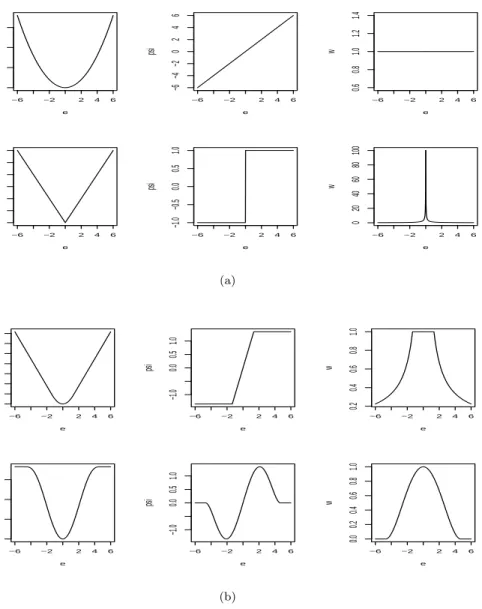
2.1 Figure (a) shows the objective,ψ, and weight functions for the least-squares(top) and LAD (bottom) estimators. Figure (b) shows the objective,ψ, and weight functions for the Huber (top) and bisquare (bottom) estimators. The tuning constants for these graphs are k=1.345 for the Huber estimator and k=4.685 for the bisquare. (One way to think about this scaling is that the standard deviation of the errors,σ, is taken as 1.) . . . 8

2.2 Least squares estimate (solid line) and M-estimate with Huber function (dashed line) for a dataset contains 20 observations two of which are high leverage outliers. . . 10

3.1 Plot of MSE of slope estimates vs. different cases for LMS, LTS, S, MM, and REWLS, for model 1 whenn= 20. . . 20

3.2 Plot of MSE of intercept estimates vs. different cases for LMS, LTS, S, MM, and REWLS, for model 1 whenn= 20 . . . 21

(6)

List of Tables

3.1 Breakdown Points and Asymptotic Efficiencies of Various Regression Estimators . . . 19

3.2 MSE of Point Estimates for Model 1 withn= 20 . . . 22

3.6 Cigarettes data . . . 27

(7)

Acknowledgments

First and foremost, I would like to express my appreciation to my major professor, Dr. Weixin Yao, for all his encouragement, guidance and suggestions.

I would also like to thank Dr. Leigh Murray and Dr. Abigail Jager for their willingness to serve on my committee and for their valuable insight.

My gratefulness extends to everyone who supported me in any respect during the completion of the report.

(8)

Chapter 1

Introduction

1.1 Least Squares estimate

The most basic method to estimate the parameters of linear regression models is theLeast Squares method

(LS method). The idea of least-squares analysis was independently formulated by Gauss (1777-1855) and Legendre (1752-1833), though it was first proposed in 1805 by Legendre (for more details, see Stigler, 1981). Since it was the only method of estimation that could be effectively computed before the advent of electronic computers, the LS method found immediate and lasting success.

Suppose the linear regression model is

y=Xβ+e, (1.1)

where yis a n×1 response variable vector,X is an×pdesign matrix, β is ap×1 unknown parameter vector andeis the random error vector. The LS estimate ofβis the ˆβ which can minmize

ky−Xβk2

Let

Q(β) =ky−Xβk2= (y−Xβ)0(y−Xβ). We can get

Q(β) =y0y−2y0Xβ+β0X0Xβ. Differentiating with respect toβyields

X0Xβ=X0y. (1.2)

The matrix equation (1.2) is called the ‘normal equations’. IfXhasf ull rankthen the solution is unique and is given by

ˆ

(9)

IfXis not of full rank, then we have what is calledcollinearity. In this situation, we will have an infinite number of solutions, which all yield the same predicted values and hence the same residuals.

The least squares estimate is optimal among the class of linear unbiased estimates and it is also the most efficient unbiased estimate under the assumption that errors in regression models are normally distributed (ei ∼IIDN(0,σ2)). However, in reality, errors do not usually exactly follow a normal distribution. Outliers

often exist in a data set or errors may follow another distribution (e.g. t-distribution which has a heavier tail than the normal distribution). Here outliers are observations which do not follow the pattern of the other observations. In either case, the LS estimator will diverge strongly from the real value, no matter how big the sample size is.

Since the LS estimate is so sensitive to outliers, the easy and popular way to improve the estimate is by modifying or deleting outliers and applying LS to the modified data. Classical methods for outlier detection are based on initial LS fit and using numerical or graphical procedures (or both) calledregression diagnostics

to detect influential observations. These include the familiar Q-Q plots of residuals, plots of residuals vs. fitted values, Cook’s distance, leverages, “leave-one-out” approach and so on. Since all of these methods are based on the initial LS fit, the residuals, standard deviations, and leverages may be largely influenced by outliers. Therefore, the above methods can be fooled by the combined action of several outliers, an effect that is referred to as masking, so these methods may even fail to recognize a single outlier.

Because of the above mentioned problems with the LS estimate, we want to develop new procedures that give a good fit to the unusual data without being perturbed by a small proportion of outliers and that do not require deciding and removing outliers. This leads torobust regression.

1.2 Robust Method

1.2.1 Background

Robust linear regression is designed to circumvent some limitations of traditional parametric methods. Ordinary least squares played an important role in the estimation field since they have favorable properties if their underling assumptions are true. Unfortunately, those assumptions are often not met in practice. When people realized this, they started to seek methods which could remedy this problem. The idea of robust methods developed at the beginning of nineteenth century, with the rapid development of electronic technology. Robust statistics have attracted increasing attention from the 1960s. Now this is a very popular research area in statistics and a large number of articles have been published. There is still considerable work that needs to be done in this research area. This paper will review some popular robust regression methods and discuss their properties.

(10)

Robust regression tries to seek a model which represents the information in the majority of the data. Usually we use the properties of efficiency, the breakdown point (Donoho, 1983), and the influence function (Hampel, 1974) to measure the performance of robust techniques. The breakdown point and influence function will be described in the next section. The efficiency tells us how well the robust method works compared to LSE when data exactly follow a normal distribution. Because LSE is the best estimation method when data are normal, we want the robust estimator to perform as closely to LSE as possible. Thus, high efficiency is desired for robust estimation.

Historically, robust regression techniques mainly deal with three classes of problems:

1) Outliers only in the response direction (y−direction)

2) High leverage outliers (outliers in both thex−spaceandy−direction) 3) Distribution with heavier tail than normal distribution

Many methods have been developed for these problems. In the last chapter of this paper, we will discuss the properties of some robust methods based on these three kinds of problems by simulation studies.

1.2.2 Measuring Robustness

The goal of robust methods is to develop estimates which have ‘good’ behavior in an approximately normal model. The most common method to measure robustness is the breakdown point. The breakdown point (BP) is the largest proportion of the contaminations that the data can contain before the estimate fails. Thus the higher the BP of an estimator, the more robust it is. A common practical definition is the BP for a finite sample (FBP). The finite sample version of this concept is given by Donoho and Huber (1983) and is defined as the following.

LetZ={(xi, yi) :i= 1,2, . . . , n} and the corresponding ˆβ=T(Z). Then the breakdown-point ofTat

Zis defined by

ε∗(T,Z) =min{m/n: sup

Z∗

kT(Z∗)−T(Z)k=∞},

where k · k denotes the Euclidean norm and the supremum is taken over all choices of Z∗ consisting of (n−m) points fromZandmarbitrary points.

It is obvious that the BP of a sample mean and LSE is _n1, since even one outlier will lead to a big change in the estimation. For a similar reason, the BP of the sample median is 1₂, which is the highest value of BP. Intuitively, a BP cannot exceed 1

2 because if more than half of the data are outliers, it is impossible to

distinguish between the “good” and “bad” distributions. Therefore, the maximum BP is 0.5 which is the goal of robust estimation. Although the sample median can achieve the best BP value, its efficiency is very low.

(11)

Another popular measurement of robustness is the influence function (Hampel, 1974). Let ˆβ be the estimate of βbased on the original data and ˆβ₀ be the estimate based on the data which has removed all outliers. Then we call ˆβ−βˆ₀thesensitivity curveof ˆβ. The influence function (IF) is an asymptotic version of the sensitivity curve. When the sample contains a small fractionεof identical outliers, it is defined as

IF_βˆ(x0, F) = lim

ε→0+ ˆ

β_∞((1−ε)F+εδx0)−βˆ∞(F)

ε ,

wherex0is the outlier, δx0 is a point mass atx0, and ˆβ∞(F) is theasymptotic value of the estimate atF. The IF is a measure of the rate at whichβresponds to a small amount of contamination atx0. Loosely

speaking, it tells us how much a single outlier affects the estimate. For a robust estimator, we want to ensure the IF does not go to infinity asxbecomes arbitrarily large. Therefore, a bounded influence function is desired.

(12)

Chapter 2

Review of Robust Regression

Methods

2.1 M-estimate

The most common general robust method is estimates, introduced by Huber (1973). The M in M-estimates stands for “maximum likelihood type”. That is because M-estimation is a generalization of maximum likelihood estimates (MLE). Suppose the regression model is

yi=x0iβ+εi, (2.1)

whereεi has a density 1_σf(_σe) andσis a scale parameter. Thenyi0shave density functions

1

σf( yi−x0iβ

σ ) and

thelikelihood function forβ andσis

L(β, σ) = n Y i=1 1 σf( yi−x0iβ σ ) = 1 σn n Y i=1 f(yi−x 0 iβ σ ). (2.2)

Based on this, the log likelihood is given by:

l(β, σ) =−nlogσ+ n X i=1 logf(yi−x 0 iβ σ ).

Setting ρ(x) =−logf(x), and lettingei(β) =yi−x0iβ, we have

l(β, σ) =−[nlogσ+ n X i=1 ρ(ei(β) σ )].

To maximize this equation is equivalent to minimizing

logσ+1 n n X i=1 ρ(ei(β) σ ). (2.3)

(13)

Assumingσis a fixed value, the M-estimator minimizes theobjective function n X i=1 ρ(ri) = n X i=1 ρ(ei(β) σ ), (2.4) where ri = ei(β)

σ are called standardized residuals. Letψ(x) = ρ

0_{(x) =}₋_f0_(x)/f_{(x), differentiating (2.4)} with respect toβ, assumingσis fixed, and setting the partial derivatives to 0, we get the normal equations

n X

i=1

ψ(ei(β)

σ )xi=0. (2.5)

To solve (2.5) we define theweight function

W(x) =    ψ(x)/x, ifx6= 0; ψ0(0), if x=0. (2.6)

and letwi=W(ri). Then equations (2.5) can be written as n

X

i=1

wi(yi−x0iβ)xi=0. (2.7)

Note that if wi is known, the above equation generates the weighted least squares estimate. For robust

estimate, usually ψ(·) is bounded. Therefore, the weights wis will be small if the standardized residuals

ris are large and thus downweight the effects of outliers. The solution of (2.7) can be found by iterating

betweenwi andβ:

1. Set an initial estimatesβ(0), for example LSEs.

2. Calculate standardized residuals r(_ik−1)and weightsw_i(k−1)=W(r_i(k−1)) at each iterationk from the previous iteration.

3. Update βby

βk = [X0W(k−1)X]−1X0W(k−1)y,

whereW(k−1)=diag{w(_ik−1)} is the current weight matrix. Repeat step 2 and step 3 until the estimated coefficients converge.

In equation (2.4), a reasonableρshould satisfy the following properties:

• ρ(e)≥0 (nonnegative);

• ρ(e) =ρ(−e) (symmetric);

• ρ(0) = 0;

(14)

Several choices of ρ have been proposed. If ρ(x) = 1

2x

2_{, then the solution of the normal equations is the}

LSE which we introduced in chapter 1. Ifρ(x) =|x|, then the objective function becomes:

n X

i=1

|ei( ˆβ)|=min.

This is known as the L1 estimate, which is also called the Least Absolute Deviation (LAD) estimate or

median regression estimate. Another two popular choices of ρ are the Huber function and the Tukey

bisquare (orbiweight) function. For the Huber function,

ρH(e) =    1 2e 2_, _for_|_e_{| ≤}_k; k|e| − 1 2k 2_, _for_|_e_|_{> k.}

The corresponding weight function is

wH(e) =    1, for|e| ≤k; k/|e|, for|e|> k. ,

where kis called atuning constant. Smaller values ofk produce more resistance to outliers, but comes at the price of loss in efficiency under the normal distribution. Usually, the tuning constant is picked to give reasonably high efficiency in the normal case, for example,k= 1.345σproduces 95% efficiency and can still offer some protection against outliers. For the Tukey bisquare function,

ρB(e) =    k2 6{1−[1−( e k) 2_]3_}_, _for_|_e_{| ≤}_k; k2_/6, _for_|_e_|_{> k.}

The corresponding weight function is

wB(e) =    [1−(e k) 2_]2_, _for_|_e_{| ≤}_k; 0, for|e|> k. Generally,k= 4.685σis used to produce 95% efficiency .

Figure 2.1 compares theρ(·),ψ(·) and weight functionsw(·) for the above four M-estimators: the familiar least squares estimate; the least absolute deviation estimate; the Huber estimate; and the Tukey bisquare estimate. The objective functions for least squares, LAD, and Huber increase without bound ase departs from 0, but the least squares objective function increases more rapidly. In contrast, the objective function for Tukey bisquare eventually levels off (for |e| > k). For weight functions, least squares assigns equal weight to each observation; the weights for the Huber estimate decline when |e|> k; and the weights for the LAD and Tukey bisquare estimators decline as soon asedeparts from 0, but LAD declines more rapidly.

(15)

−6 −2 2 4 6 0 5 10 15 e rho −6 −2 2 4 6 −6 −4 −2 0 2 4 6 e psi −6 −2 2 4 6 0.6 0.8 1.0 1.2 1.4 e w −6 −2 2 4 6 0 1 2 3 4 5 6 e rho −6 −2 2 4 6 −1.0 −0.5 0.0 0.5 1.0 e psi −6 −2 2 4 6 0 20 40 60 80 100 e w (a) −6 −2 2 4 6 0 1 2 3 4 5 6 7 e rho −6 −2 2 4 6 −1.0 0.0 0.5 1.0 e psi −6 −2 2 4 6 0.2 0.4 0.6 0.8 1.0 e w −6 −2 2 4 6 0 1 2 3 e rho −6 −2 2 4 6 −1.0 0.0 0.5 1.0 e psi −6 −2 2 4 6 0.0 0.2 0.4 0.6 0.8 1.0 e w (b)

Figure 2.1: Figure (a) shows the objective, ψ, and weight functions for the least-squares(top) and LAD (bottom) estimators. Figure (b) shows the objective,ψ, and weight functions for the Huber (top) and bisquare (bottom) estimators. The tuning constants for these graphs are k=1.345 for the Huber estimator and k=4.685 for the bisquare. (One way to think about this scaling is that the standard deviation of the errors,σ, is taken as 1.)

(16)

The above calculations are based on the assumption thatσis known. However, in reality, σis usually unknown. In this situation, we can compute it simultaneously by adding a scale M-estimating equation to equation (2.5). Differentiating (2.3) with respect to σcan get 1_nPn

i=1ρscale( ei(β)

ˆ

σ ) = 1, where ρscale(t) =

tψ(t). Thus, in general, an M-estimate of scale is the estimate which satisfies an equation of the form

1 n n X i=1 ρ(ei(β) ˆ σ ) =δ,

whereρis a ρ-function andδis a positive constant.

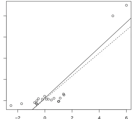
M-estimators with Huber function or Tukey bisquare function are robust to outliers in the response variable with high efficiency. However, M-estimators are just as vulnerable as least squares estimates to high leverage outliers. In fact, the BP (breakdown point) of M-estimates is 1/n → 0 (Rousseeuw and Yohai 1984). Figure 2.2 illustrates an effect of high leverage outliers on the least squares estimator and M-estimators. It shows that both methods are very sensitive to high leverage outliers.

2.2 Least Median of Squares estimate

Since M-estimators are not robust to high-leverage outliers, we want to find some methods that can have high BP. Siegel (1982) defined theleast median of squares (LMS) estimator as

min β medi {e

2

i}, (2.8)

which replaced the sum by the median in the LSE. This proposal is essentially based on an idea by Hampel (1975).

The advantage of LMS estimate is that it is very robust to outliers in both the y direction and the leverage points and it has been shown that LMS has the highest possible BP of 0.5. Unfortunately, it has a very low efficiency and it can be unstable. Moreover, due to its slow convergence rate ofn−13, LMS estimate does not have a well-defined influence function. Because of these properties, LMS estimate is usually used as the initial estimate of the residuals for other more efficient methods such as MM-estimators (Yohai, 1987).

2.3 Least Trimmed Squares estimate

Another regression estimator that has BP of nearly 50 percent is theleast trimmed squares (LTS) estimator proposed by Rousseeuw and Yohai (1984). This estimator chooses the regression coefficientsβto minimize the sum of the smallesthof the squared residuals and is defined as:

ˆ β_{LT S} = arg min β h X i=1 e2₍_i₎(β), (2.9)

(17)

● ● ● ● ● ● ● ● ● ● ●● ● ● ● ● ● ● ● ● −2 0 2 4 6 0 10 20 30 40 x y

Figure 2.2: Least squares estimate (solid line) and M-estimate with Huber function (dashed line) for a dataset contains 20 observations two of which are high leverage outliers.

where e2

(i)(β) represents the i−th ordered squared residuals e 2

(1)(β) ≤. . . ≤e 2

(n)(β) and h is called the

trimming constant which has to satisfyn₂ < h≤n. This constanthdetermines the BP of the LTS estimator. Typically, h=bn/2c+b(p+ 1)/2ccan attain the maximum BP = (b(n−p)/2c+ 1)/n, where b cmeans rounding down to the next smallest integer. Whenh=n, LTS is exactly equivalent to LS estimator whose BP is 0. Like LMS, LTS has a high BP but low efficiency. Although its convergence rate ofn−12 (Rousseeuw 1983) makes it asymptotical normal which is better than LMS, it still suffers a very low efficiency of only 7%. The reason that LTS estimator is discussed in this paper is that LTS is often suggested as the starting point for more efficient procedures.

(18)

2.4 S-estimate

To find a simple high-breakdown regression estimator which shares the flexibility and nice asymptotic properties of M-estimator, Rousseeuw and Yohai (1984) introduced the estimator. They called it S-estimator because it is derived from the M-scale estimate equation:

1 n n X i=1 ρ(ei(β) ˆ σ ) =δ. (2.10)

In M-estimates, when σ is unknown, we use this equation with equation (2.5) to get the scale parameter and regression parameter simultaneously. Letδ=EΦ[ρ(x)], where Φ represents the standard normal, and

let

d(e) = #{i: 1≤i≤n, ei= 0}/n.

When d(e)<1−δ/a (wherea is the upper bounded of ρand a ∈(0,∞)), equation (2.10) has a unique positive solution; ifd(e) = 1−δ/a, equation (2.10) may have infinite solutions which includeσ= 0; and if d(e)>1−δ/a, then no solution for equation (2.10) exists. To avoid indeterminacies, we combine the last two situations together and define wheneverd(e)≥1−δ/a,σ(e) = 0.

To define S-estimator we letρsatisfy (A1):

(i) symmetric, continuously differentiable andρ(0) = 0;

(ii) there existsc >0 such thatρscaleis strictly increasing on [0, c] and constant on [c,∞).

For each vector β, using (2.10) we can calculate the dispersion of residuals ˆσ(e1(β), . . . , en(β)), where ρ

satisfies (A1). Then the S-estimator ˆβis defined by

arg min

β σ(eˆ 1(β), . . . , en(β)). (2.11) The breakdown point of S-estimator can be made to obtain 0.5 with an appropriateρ-function. A popular choice of ρ-function is the bisquare (or biweight) function:

ρ(x) =    x2 2 − x4 2k2 + x6 6k4, for|x| ≤k; k2 6, for|x|> k. (2.12)

Whenk = 1.547, BP is equal to 0.5 but at the cost of low efficiency which is only 28.7%. Hossjer (1992) proved that there exists a trade-off between efficiency and robustness. In other words, S-estimator cannot achieve simultaneously high breakdown point and high efficiency under the normal model. To make up this, we chose the S-estimator with high breakdown point as the initial estimator for the one-step M-estimator (Bickel 1975), so that the resulting one-step M-estimator has high efficiency and also inherits the 0.5 BP from the first stage (more details in Chapter 2.7).

(19)

2.5 τ

-estimate

As shown above, some estimates might have a high breakdown point, but at the cost of low efficiency under normal errors. To solve this problem, Yohai and Zamar (1988) defined a broader class of scale estimates, called τ-estimate, and singled out a subclass that can achieve a high BP and high efficiency at the same time.

Letρandρ1be two bounded continuousρ-function, and let ˆσ(e) be a robust M-scale estimate based on

ρ. Then lete= (e1, . . . , en) and define the scaleτ as

τ2(e) = ˆσ2(e)1 n n X i=1 ρ1( ei ˆ σ(e)). (2.13)

Then the regressionτ-estimate ˆβis defined by

arg min

β τ(e(β)). (2.14)

Yohai and Zamar (1988) showed that the BP depends only onρ. Therefore, we choose an appropriate ρ satisfying all the assumptions so that the τ estimator has a high BP, and at the same time, choose a ρ1 so that the τ estimator has arbitrarily high efficiency under the normal model. It is also shown that

by adequately choosing ρand ρ1, the estimate can attain the maximum BP (0.5) for regression estimates

and arbitrarily efficient at the normal distribution (close to 1). For example, when the bisquare family ofρ function (2.12) is used, if we take k= 1.56 andEΦ(ρ) = 0.203 for ρand k1 = 6.08 for ρ1, the resultingτ

estimator has simultaneously a breakdown point of 0.5 and an efficiency of 0.95 under normal distribution. The computing algorithm of this estimate is a modification of the iterative weighted least squares algo-rithm for M estimates (see Yohai and Zamar, 1988). And in that paper, they also showed that aτ estimate is asymptotical equivalent to an M estimate with a ψ function given by a linear combination of ρ0 andρ0₁ with coefficients depending on the data.

2.6 M M-estimate

Another class of robust estimates which have high breakdown point and high efficiency under normal error is MM-estimates. Yohai (1987) introduced the MM-estimates for robust regression. This estimate is defined in three stages:

STAGE 1. Compute an initial consistent robust estimate ˆβ₀with high BP, possibly 0.5, but not necessarily efficient.

STAGE 2. Compute the M-scale ˆσ of the residuals ei( ˆβ0) using equation (2.10), using a function ρ0

satisfying (A1) and choosing a constant δ such that δ/a = 0.5, where a = supρ0(e). Thus, the

(20)

STAGE 3. Letρ1be anotherρ-function satisfying (A1) and such that

supρ1(e) = supρ0(e) =a, (2.15)

ρ1(e)≤ρ0(e). (2.16) Letψ1=ρ01,L(β) = Pn i=1ρ1( ei(β) ˆ

σ ), andρ1(0/0) = 0. Then the MM-estimate ˆβ1 is defined as any

solution to the equation

n X i=1 ψ1( ei(β) ˆ σ )xi =0, (2.17)

that also satisfies

L( ˆβ₁)≤L( ˆβ₀). (2.18)

Yohai (1987) showed that any value ofβwhich satisfies (2.17) and (2.18), e.g., a local minimum, will have the same efficiency as the global minimum and its BP is not less than that of ˆβ₀. Thus, although the absolute minimum ofL(β) exists, it is not necessary to find it.

In the first stage, the robust initial estimate ˆβ₀should satisfy regression, scale and affine equivalent and also have a high BP. LMS-, LTS-, and S-estimates are possible candidates. For stage 2, one way of choosing ρ0andρ1 is as follows. Letρbe a function satisfying (A1) and letρ0(e) =ρ(e/k0) andρ1(e) =ρ(e/k1). In

order to satisfy (2.16), we must have 0 < k0 < k1. The value of k0 should be chosen such thatδ/a= 0.5

holds. It has also been proven that the asymptotic variance of MM-estimate depends only onk1: the larger

k1, the higher the efficiency at the normal distribution. Therefore, similarly toτ-estimate, MM-estimate can

attain high efficiency by choosing an appropriatek1 without affecting its breakdown point, which depends

only on the choice ofk0. For example, letρbe theρ-function of bisquare family (2.12) andk0= 1.56 which

can hold the equations in stage 2, the correspondingδ= 0.0833 andk1= 4.68 which gives efficiency 0.95 for

normal errors. However, Maronna, Martin, and Yohai (2006) showed that there is a basic trade-off between normal efficiency and bias under contamination and Yohai (1987) also indicated that MM-estimates with larger values of k1 are more sensitive to outliers than the estimates corresponding to smaller values of k1.

It is therefore important to choose the efficiency to balance these. Maronna, Martin, and Yohai (2006) recommended the efficiency of 0.85 which gives a small bias while retaining a sufficiently high efficiency. And for the above example, this requirek1= 3.44 which is a smaller value compare to 4.86.

The numerical computation of MM-estimate is a modified version of the IRWLS (iterated weighted least-squares) algorithm used for computing M-estimate. First we define the weight function fort∈Rp_:

wi(t) = ψ1(ei(t)/ˆσ) ei(t)/ˆσ . (2.19) Also define g(t)= 1 ˆ σ2 n X i=1 wi(t)ri(t)xi, (2.20)

(21)

and M(t)= 1 ˆ σ2 n X i=1 wi(t)xix0i, (2.21)

where−g(t)is the gradient ofL(t). To ensure (2.18) holds, we modify IRWLS as follows: take 0< δ <1, and find an integerk such that

L(t(j)+ ∆(t(j))/2k)≤L(t(j))−δ(∆(t(j))/2k)0g(t(j)), (2.22) where ∆(t) =M−1(t)g(t). Letk1,j be the minimum of such k0s, 0≤k≤k1,j, and letk2,j be the value of

kwhich gives the minimum ofL(t(j)+ ∆(t(j))/2k). Then the recursion step is defined by

t(j+1)=t(j)+ (1/2k2,j_)∆(t(j)_), _(2.23)

starting witht(0)_{= ˆ}_β

0. Thus any limit point of the sequencet

(j)

is an MM-estimate.

2.7 GM-estimate

The M-estimate is the most popular robust estimate but it has a low BP due to the failure to account for high leverage outliers. In response to this problem, bounded influence generalized M estimate (GM estimate) were proposed to produce stable results when there are outliers in the explanatory variables. Examples of these proposals include Mallows (1975), Hampel (1978), Krasker (1980), and Krasker and Welsch (1982). The goal of GM-estimate is to create weights that consider the outliers both in the y-direction and the leverage points. Using a standard M-estimate to deal with the vertical outliers, the weight functions can downweight leverage points so that observations with high leverage receive less weight than observations with small leverage. The general GM class of estimators is defined by

n X i=1 wi(xi)ψ{ ei( ˆβ) v(xi)ˆσ }xi= 0, (2.24)

whereψ is the score function (as in the case of M-estimate).

2.7.1 Mallows GM-estimate

The first GM-estimate was proposed by Mallows (1975). For Mallows GM-estimate, the vi in equation

(2.24) is equal to 1 and wi =

√

1−hi where hi is the hat value. Hat values range from 0 to 1, so weight

function downweights the high leverage points. However, there are possible leverage points whose responses fall in line with the pattern in the bulk of the data. In these cases Mallows GM-estimate cannot distinguish these “good” leverage points and will down weight them which result in a loss of efficiency.

(22)

2.7.2 Schweppe GM-estimate

Another GM-estimate is called Schweppe GM-estimate. This method adjusted the leverage weights accord-ing to the size of the residual ei by using vi = wi, where wi is the weight function which is the same as

Mallows GM-estimate and equal to√1−hi(see Handschin et al. 1975). However, since the weight function

of this estimate only depends onxvalues without considering how the correspondingy values fit with the pattern of the bulk of the data, efficiency is still hindered (Krasker and Welsch 1982). Moreover, Carroll and Welsh (1988) suggested that the Schweppe estimate is not consistent when the errors are asymmetric. The breakdown points for the above two GM-estimates, although better than for regular M-estimate, are at most 1/(p+ 1), where p is the number of predictor variables (Maronna, Bustos and Yohai 1979). Thus, as dimensionality increases, their BP tends to 0.

2.7.3 One-step GM-estimate

We usually refer to the property of high BP as global stability and that of bounded influence as local stability. To combine these two stabilities as well as a degree of efficiency under the Gauss-Markov assumptions, one-step GM estimate was proposed by several authors (Bickel, 1975; Jureckova and Portnoy, 1987; Giltinan, Carroll, and Ruppert, 1986). The strategy of this estimate is as follows: Start with a high breakdown point estimator such as LTS or LMS and perform one iteration towards solution of the GM-estimate equations. And it takes the form

ˆ

β= ˆβ₀+H₀−1g0, (2.25)

where ˆβ₀is a high breakdown preliminary estimate with BP at leastm/n(usually we takem= [(n−p)/2] + 1), g0= ˆσ0P

n

i=1Ψ(ei/ˆσ0)wixi. There are two viable choices forH0:

• Newton-Raphson: H0=P n i=1wixix0iψ(1)(ei/σˆ0); • Scoring: H0=n−1P n i=1ψ (1)_(e i/σˆ0)P n j=1wjxjx0j.

These two methods are asymptotically equivalent if the errors are independent, identically and symmetrically distributed. Forwi, we use Mallows weights:

wi=min[1,

b

(xi−mx)0Cx−1(xi−mx) α/2

]

and set b equal to the (1−r) quartile of the chi-squared distribution with df =p−1, where r = 0.1 or 0.5. In the formula, whenα= 0, we call it one-step Huber estimate which is discussed by Bickel (1975) and Jureckova and Portnoy (1987); whenα= 1, we usually use it for GM estimate; and when α= 2, Giltinan, Carroll and Ruppert (1986) used it to force a bounded change of variance.

Simpson, Ruppert, and Carroll (1992) showed that under reasonably general conditions, one-step Mallows estimates inherit the breakdown properties of the preliminary estimates of the regression parameters and

(23)

the multivariate location and scale estimates of the design x’s. However, the estimated standard errors of this estimate may change radically with deletion of a single observation.

2.8 Robust and Efficient Weighted Least Squares estimate

In the model (1.1), we assume the error terms {ei} are iid unobservable random variables with unknown

distributionF0(_σ·) for some scale parameterσ >0. F0 is symmetric about 0.

Let ˆβ0 and ˆσ0 be the initial robust estimators of regression and scale, respectively. If ˆσ0 > 0, the

standardized residuals defined in Chapter 2.1 are:

ri=

yi−x0iβˆ0

ˆ σ0

. (2.26)

Then, a large |ri| implies that (xi, yi) is an outlier. The idea of weighting is: we set a cutoff point say

t0, if |ri| ≤ t0 we will keep that point, but if |ri| > t0 we will treat it as an outlier and remove it by

weighting it 0. As we know that this weighting step improves the efficiency under normal errors and also maintains the breakdown point of the initial estimator. However, He and Portnoy (1992) showed that, it cannot be asymptotically efficient. To obtain the full asymptotic efficiency under normal errors without less the breakdown point of the initial estimator, Gervini and Yohai (2002) suggested using the adaptive cutoff values which lead to a new class of estimators calledrobust and efficient weighted least squares estimators

(REWLSEs). Instead of setting a particular fixed value tot0, this method adaptively calculatestnfrom the

data.

To define the adaptive cutoff values, first let the empirical distribution function of the standardized absolute residuals be F_n+(t) = 1 n n X i=1 I(|ri| ≤t). (2.27)

Suppose the distribution function of the absolute errors under the actual model isF₀+(t). IfFn+(t)< F

+

0 (t)

under a large t, then we can say there are outliers in the sample. However, in reality, we will never know the actual distribution of the errors, so a hypothetical F = Φ must be used instead of F0. Secondly, we

define a measure of the proportion of outliers in the sample:

dn= max i>i0 {F+(|r|(i))− i n} +_, _(2.28)

where{·}+_{denotes the positive part,}_F+_{denotes the distribution of}_|_X_|_when_X_∼_{F. Let}_|_r_|

(1)≤...≤ |r|(n)

be the order statistics of the standardized absolute residuals. Theni0= max{i:|r|(i)< η}. Hereη is some

large quartile ofF+(Rousseeuw and Leroy (1987) usedη= 2.5). Thus thosebndncobservations (herebndnc

is the largest integer less than or equal to ndn) with largest standardized absolute residuals are eliminated

(24)

adaptive cut-off value is:

tn =min{t:Fn+(t)≥1−dn}, (2.29)

which means the same thing as above. With thistn,we define weights of the form wi=w(|ri|/tn). When

w(u) =I(u <1) we called it thehard-rejection weight which is the most common weight function. However, in general, we will only require w(u) to satisfy the following three properties:

1)w(0) = 1. 2)    w(u)>0, if 0< u <1; w(u) = 0, ifu≥1.

3)u∈[0,∞), w(u)∈[0,1], w(u) is nonincreasing, right continuous and continuous in a neighborhood of 0.

The property 2) ensures that observations with large residuals are completely eliminated. LetW=diag(w1,...,wn)

andY=(y1,...yn)

0

,REWLSE is defined as:

ˆ β_{REW LSE} = ˆβ₁=    (X0WX)−1_X0_WY, _{if ˆ}_σ 0>0; ˆ β₀, if ˆσ0= 0.

Gervini and Yohai (2002) showed thattnremains bounded in the presence of outliers which implies that

ˆ

β1keeps the finite sample and asymptotic breakdown points of ˆβ0. They proved that the BP of REWLSE

satisfies ε∗

n( ˆβ1,Z) ≥ εn∗( ˆβ0,Z)−1/n . On the other hand, the REWLS estimates are asymptotically

equivalent to the LS estimates and hence asymptotically efficient under the normal errors. That is because when F0 is of unbounded support but of lighter tails thanF, its cutoff value will approach infinity under

the model and thenw(|ri|/tn)→1. The same happens if F0 is of bounded support with lighter tails than

(25)

Chapter 3

Comparing Various Estimators

Table 3.1 summarizes the robustness and efficiency attributes of most of the estimators we have discussed in Chapter 2. The breakdown point, whether or not the estimator has a bounded influence function, and the approximate asymptotic efficiency of the estimator relative to the LSE are reported. When compared in terms of breakdown point, it is obvious that M-estimate and LAD have the BP as low as LSE which indicates a single discrepant observation can render these estimates useless. Sometimes the LAD and M-estimate perform no better than LSE. Although GM-M-estimate has a higher BP, however, when the number of parameters increase, its BP can be very small. On the other hand, when looking at the high BP estimates we should also be cautious of the low efficiency. Here, LMS, LTS, and S-estimates have asymptotic efficiency less than 0.4. When used in combination with more resistant estimators,τ-estimate, MM-estimate, one-step GM-estimate, and REWLS-estimate can attain a nearly optimal efficiency and maximum breakdown point at the same time.

3.1 Simulation Study

According to the various types of outliers introduced in Chapter 1, we now compare different methods and report the mean squared errors (MSE) of the parameter estimates for each estimation method. We explore eight different regression estimates: LSE, M-estimate using Huber weights (MH), M-estimate using Tukey

weights (MT), LMS, LTS, S-estimate, MM-estimate (using bisquare weights andk1 = 4.68), and REWLS.

We use two models to compare the performance of these eight methods:

Model 1:

Y =X+ε,

(26)

Table 3.1: Breakdown Points and Asymptotic Efficiencies of Various Regression Estimators

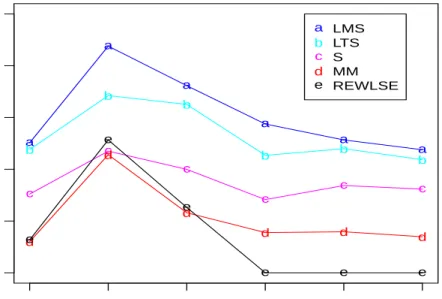
Estimator Breakdown Point Bounded Asymptotic Efficiency

High BP LMS 0.5 Yes 0 LTS 0.5 Yes 0.07 S-estimates 0.5 Yes 0.29 τ-estimates 0.5 Yes 0.95 MM-estimates 0.5 Yes 0.85 GM-estimates(one-step) 0.5 Yes 0.95 REWLS-estimates 0.5 No 1.00

Low BP GM-estimates(Mallows,Schweppe) 1/(p+ 1) Yes 0.95

M-estimates 1/n No 0.95

LAD 1/n No 0.64

LSE 1/n No 1.00

Model 2:

Y =X1+X2+X3+ε,

whereXi∼N(0,1), i= 1,2,3 andXis are independent.

We consider the following six cases for the error density ofε: Case I:ε∼N (0,1)- standard normal distribution.

Case II:ε∼t1 - t-distribution with degrees of freedom 1 (Cauchy distribution).

Case III:ε∼t3- t-distribution with degrees of freedom 3.

Case IV:ε∼N (0,1) with 10% identical outliers iny direction (where we let the first 10% ofy0_s_equal to 30).

Case V:ε∼N (0,1) with 10% identical high leverage outliers (where we let the first 10% ofx0sequal to 10 and their correspondy0sequal to 50).

Case VI:ε∼0.95N (0,1) + 0.05N (0,102_{) - contaminated normal mixture.}

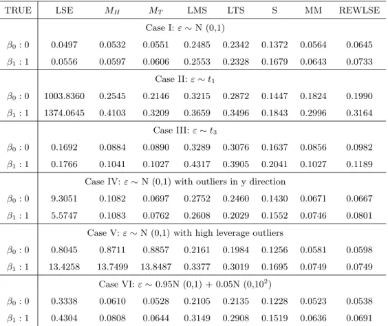
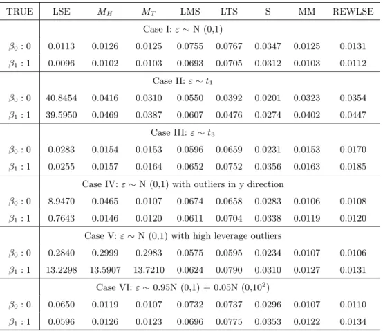
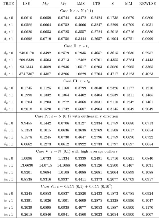
For each of those we use R to simulate 200 samples and get the mean squared errors of the parameter estimates for each estimation method. Table 3.2 and 3.3 show the mean squared errors (MSE) for model 1 and sample size n=20 and n=100, respectively; Table 3.4 and 3.5 show the mean squared errors (MSE) for model 2 and sample size n=20 and n=100, respectively. Based on these four tables, we can see that MM-estimates and REWLS estimates have the overall best performance throughout most cases and they are consistent for different sample sizes. For Case I, LSE has the smallest MSE which is reasonable since under normal errors LSE is the best estimate; M-estimates, MM-estimate, and REWLS estimate have similar MSE to LSE, due to their high efficiency property; LMS, LTS, and S estimate have relative larger MSE

(27)

due to their low efficiency. For Case II, it can be seen that LSE has much larger MSE than other robust estimators; M-estimates, MM-estimate and REWLS estimate have similar MSE to S-estimate. For Case III, M-estimate, MM-estimate, and REWLS work better than other estimates. From Case IV, we can see that when the data contain outliers in the y-direction, LSE is much worse than any other robust estimates; MM-estimates, REWLS, andMT are better than other robust estimators. For Case V, since there are high

leverage outliers, similar to LSE, bothMT andMHperform poorly; MM-estimate and REWLS work better

than other robust estimates for this case. Finally for Case VI, M-estimates, MM-estimate, and REWLS estimates have smaller MSE than others.

In summary, LSE only works well when there are no outliers since it is very sensitive to outliers. M-estimates (MH andMT) work well if the outliers are iny direction but is also sensitive to the high leverage

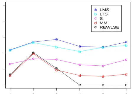
outliers. To better compare the performance of LMS, LTS, S, MM, and REWLS, Figure 3.1 and Figure 3.2 show the plot of their MSE versus each case for slope and intercept parameters, respectively, for model 1 when n = 20. Since the lines for LTS and LMS estimates are above the other lines, we conclude that S-estimate, MM-estimate, and REWLS are better estimates than LTS and LMS. In addition, it seems that REWLS has the overall best performance and MM-estimate has overall better performance than S-estimate. Plot for intercept tells a similar story.

1 2 3 4 5 6 0.0 0.1 0.2 0.3 0.4 0.5

Cases vs. MSE for slope

Case MSE a a a a a a b b b b b _b c c c c c _c d d d d d _d e e e e e e a b c d e LMS LTS S MM REWLSE

Figure 3.1: Plot of MSE of slope estimates vs. different cases for LMS, LTS, S, MM, and REWLS, for model 1 whenn= 20.

(28)

1 2 3 4 5 6 0.0 0.1 0.2 0.3 0.4 0.5

Cases vs. MSE for intercept

Case MSE _a a a a _a a b b b b b b c c c c _c c d d d d _d d e e e e e e a b c d e LMS LTS S MM REWLSE

Figure 3.2: Plot of MSE of intercept estimates vs. different cases for LMS, LTS, S, MM, and REWLS, for model 1 when n= 20

3.2 Example

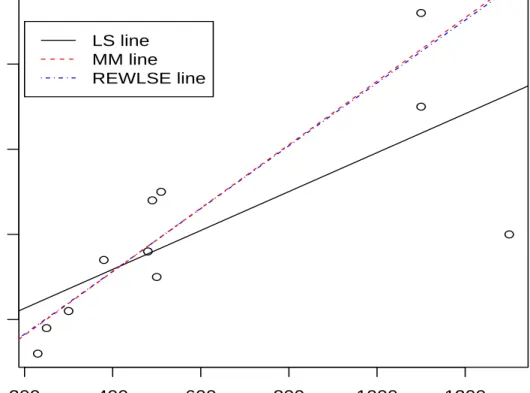
Table 3.6 shows a famous data set found in Freedman et al. (1991). The data set contains per capita consumption of cigarettes in various countries in 1930 and the death rates (number of deaths per million people) from lung cancer for 1950. We let death rates per million people be the dependent variable y and let the consumption of cigarette per capita be the independent variable x. The previous study indicates that the data for USA is an outlier. Figure 3.3 is a scatter plot of the data. From the plot, we can see that USA is an outlier with high leverage. Here, let’s compare LSE with MM-estimate and REWLS. Figure 3.3 shows the data and the lines fit by these three estimate. The LSE line does not fit the bulk of the data, being a compromise between USA data and the rest, while the fitted lines for the other two estimates almost overlap and give a better representation of the majority of the data.

Table 3.7 also gives the estimated parameters for these three methods with the complete data and with the points of USA deleted. Comparing these two cases, For LSE the intercept estimate changes from 67.56 (whole data set) to 9.14 (without outlier) and the slope estimate changes from 0.23 (whole data set) to

(29)

Table 3.2: MSE of Point Estimates for Model 1 withn= 20

TRUE LSE MH MT LMS LTS S MM REWLSE

Case I:ε∼N (0,1) β0: 0 0.0497 0.0532 0.0551 0.2485 0.2342 0.1372 0.0564 0.0645 β1: 1 0.0556 0.0597 0.0606 0.2553 0.2328 0.1679 0.0643 0.0733 Case II:ε∼t1 β0: 0 1003.8360 0.2545 0.2146 0.3215 0.2872 0.1447 0.1824 0.1990 β1: 1 1374.0645 0.4103 0.3209 0.3659 0.3496 0.1843 0.2996 0.3164 Case III:ε∼t3 β0: 0 0.1692 0.0884 0.0890 0.3289 0.3076 0.1637 0.0856 0.0982 β1: 1 0.1766 0.1041 0.1027 0.4317 0.3905 0.2041 0.1027 0.1189

Case IV:ε∼N (0,1) with outliers in y direction

β0: 0 9.3051 0.1082 0.0697 0.2752 0.2460 0.1430 0.0671 0.0667

β1: 1 5.5747 0.1083 0.0762 0.2608 0.2029 0.1552 0.0746 0.0801

Case V:ε∼N (0,1) with high leverage outliers

β0: 0 0.8045 0.8711 0.8857 0.2161 0.1984 0.1256 0.0581 0.0598

β1: 1 13.4258 13.7499 13.8487 0.3377 0.3019 0.1695 0.0749 0.0749

Case VI:ε∼0.95N (0,1) + 0.05N (0,102)

β0: 0 0.3338 0.0610 0.0528 0.2105 0.2135 0.1228 0.0523 0.0538

β1: 1 0.4304 0.0808 0.0644 0.3149 0.2908 0.1519 0.0636 0.0691

0.37 (without outlier). Thus, it is clear that the outlier strongly influences LSE. For MM-estimate, after deleting the outlier, the intercept estimate change slightly but slope estimate remains almost the same. For REWLSE, both intercept and slope estimates remain unchanged after deleting the outlier. In addition, note that REWLSE for the whole data gives almost the same result as LSE without the outlier.

(30)

Case I:ε∼N (0,1) β0: 0 0.0113 0.0126 0.0125 0.0755 0.0767 0.0347 0.0125 0.0131 β1: 1 0.0096 0.0102 0.0103 0.0693 0.0705 0.0312 0.0103 0.0112 Case II:ε∼t1 β0: 0 40.8454 0.0416 0.0310 0.0550 0.0392 0.0201 0.0323 0.0354 β1: 1 39.5950 0.0469 0.0387 0.0607 0.0476 0.0274 0.0402 0.0447 Case III:ε∼t3 β0: 0 0.0283 0.0154 0.0153 0.0596 0.0659 0.0231 0.0153 0.0170 β1: 1 0.0255 0.0157 0.0164 0.0652 0.0752 0.0356 0.0163 0.0185

β0: 0 8.9470 0.0465 0.0107 0.0674 0.0658 0.0283 0.0106 0.0108

β1: 1 0.7643 0.0146 0.0120 0.0611 0.0704 0.0338 0.0119 0.0120

β0: 0 0.2840 0.2999 0.2983 0.0575 0.0595 0.0234 0.0107 0.0106

β1: 1 13.2298 13.5907 13.7210 0.0624 0.0790 0.0310 0.0127 0.0131

Case VI:ε∼0.95N (0,1) + 0.05N (0,102)

β0: 0 0.0650 0.0119 0.0107 0.0732 0.0737 0.0296 0.0107 0.0110

(31)

Case I:ε∼N (0,1) β0: 0 0.0610 0.0659 0.0744 0.3472 0.2424 0.1738 0.0679 0.0800 β1: 1 0.0588 0.0664 0.0752 0.4066 0.3247 0.2299 0.0709 0.1051 β2: 1 0.0620 0.0653 0.0725 0.3557 0.2724 0.2018 0.0716 0.0880 β3: 1 0.0698 0.0719 0.0758 0.3444 0.2657 0.1904 0.0751 0.0999 Case II:ε∼t1 β0: 0 248.0170 0.3492 0.2579 0.7935 0.4657 0.3615 0.2630 0.2957 β1: 1 209.8339 0.4503 0.3713 1.2482 0.9701 0.4355 0.3784 0.4443 β2: 1 93.1344 0.4089 0.2936 1.0517 0.6203 0.5086 0.2965 0.3365 β3: 1 374.7307 0.4387 0.3206 1.0829 0.7704 0.4717 0.3123 0.4023 Case III:ε∼t3 β0: 0 0.1745 0.1125 0.1168 0.3799 0.3040 0.2326 0.1177 0.1210 β1: 1 0.1998 0.1332 0.1364 0.4402 0.3404 0.2539 0.1311 0.1485 β2: 1 0.1704 0.1203 0.1272 0.4868 0.3831 0.2118 0.1242 0.1461 β3: 1 0.2018 0.1520 0.1732 0.5687 0.4964 0.3145 0.1649 0.2049

β0: 0 9.9455 0.1442 0.0706 0.3127 0.2334 0.1759 0.0680 0.0713

β1: 1 5.1353 0.1015 0.0636 0.3638 0.2769 0.1508 0.0617 0.0654

β2: 1 5.1578 0.1245 0.0730 0.4647 0.2796 0.1759 0.0690 0.0722

β3: 1 6.0662 0.1273 0.0612 0.3922 0.2733 0.1797 0.0597 0.0654

β0: 0 1.0096 1.0733 1.1334 0.3339 0.2491 0.1716 0.0821 0.0840 β1: 1 13.6630 14.0715 14.1688 0.4698 0.3126 0.2500 0.1467 0.1031 β2: 1 0.9201 0.9684 1.0108 0.4088 0.2681 0.2064 0.0899 0.1088 β3: 1 0.8538 0.9316 0.9937 0.4411 0.3373 0.2077 0.0709 0.0957 Case VI:ε∼0.95N (0,1) + 0.05N (0,102₎ β0: 0 0.3245 0.0853 0.0837 0.2820 0.2433 0.1873 0.0785 0.0924 β1: 1 0.3391 0.1026 0.1001 0.4609 0.2875 0.2328 0.0996 0.1047 β2: 1 0.3039 0.0898 0.0938 0.4077 0.3053 0.1887 0.0900 0.1170 β3: 1 0.2618 0.0846 0.0941 0.4560 0.3023 0.2054 0.0900 0.1007

(32)

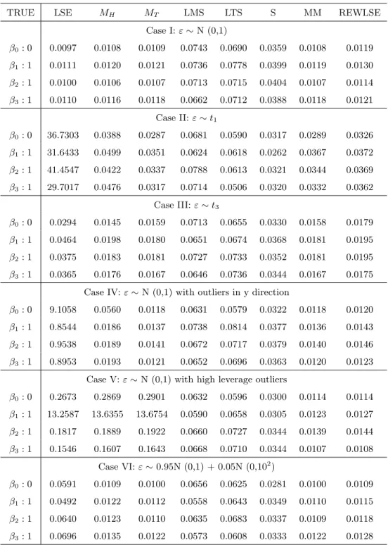
Case I:ε∼N (0,1) β0: 0 0.0097 0.0108 0.0109 0.0743 0.0690 0.0359 0.0108 0.0119 β1: 1 0.0111 0.0120 0.0121 0.0736 0.0778 0.0399 0.0119 0.0130 β2: 1 0.0100 0.0106 0.0107 0.0713 0.0715 0.0404 0.0107 0.0114 β3: 1 0.0110 0.0116 0.0118 0.0662 0.0712 0.0388 0.0118 0.0121 Case II:ε∼t1 β0: 0 36.7303 0.0388 0.0287 0.0681 0.0590 0.0317 0.0289 0.0326 β1: 1 31.6433 0.0499 0.0351 0.0624 0.0618 0.0262 0.0367 0.0372 β2: 1 41.4547 0.0422 0.0337 0.0788 0.0613 0.0321 0.0344 0.0369 β3: 1 29.7017 0.0476 0.0317 0.0714 0.0506 0.0320 0.0332 0.0362 Case III:ε∼t3 β0: 0 0.0294 0.0145 0.0159 0.0713 0.0655 0.0330 0.0158 0.0179 β1: 1 0.0464 0.0198 0.0180 0.0651 0.0674 0.0368 0.0181 0.0195 β2: 1 0.0375 0.0183 0.0181 0.0727 0.0733 0.0352 0.0181 0.0195 β3: 1 0.0365 0.0176 0.0167 0.0646 0.0736 0.0344 0.0167 0.0175

β0: 0 9.1058 0.0560 0.0118 0.0631 0.0579 0.0322 0.0118 0.0120

β1: 1 0.8544 0.0186 0.0137 0.0738 0.0814 0.0377 0.0136 0.0143

β2: 1 0.9538 0.0189 0.0141 0.0672 0.0717 0.0379 0.0140 0.0146

β3: 1 0.8953 0.0193 0.0121 0.0652 0.0696 0.0363 0.0120 0.0123

β0: 0 0.2673 0.2869 0.2901 0.0632 0.0596 0.0300 0.0114 0.0114 β1: 1 13.2587 13.6355 13.6754 0.0590 0.0658 0.0305 0.0123 0.0127 β2: 1 0.1817 0.1889 0.1922 0.0660 0.0727 0.0344 0.0139 0.0144 β3: 1 0.1546 0.1607 0.1643 0.0668 0.0710 0.0344 0.0107 0.0108 Case VI:ε∼0.95N (0,1) + 0.05N (0,102₎ β0: 0 0.0591 0.0109 0.0100 0.0656 0.0625 0.0281 0.0100 0.0109 β1: 1 0.0492 0.0122 0.0112 0.0558 0.0643 0.0349 0.0110 0.0115 β2: 1 0.0640 0.0123 0.0110 0.0635 0.0683 0.0337 0.0109 0.0118 β3: 1 0.0696 0.0135 0.0122 0.0573 0.0608 0.0333 0.0122 0.0128

(33)

● ● ● ● ● ● ● ● ● ● ● 200 400 600 800 1000 1200

100

200

300

400

Cigarettes per capita in 1930

Death b

y lung cancer in 1950

LS line MM line REWLSE line

(34)

Table 3.6: Cigarettes data

Country Cigarette per capita Deaths p. mill.

Australia 480 180 Canada 500 150 Denmark 380 170 Finland 1100 350 GreatBritain 1100 460 Iceland 230 060 Netherlands 490 240 Norway 250 090 Sweden 300 110 Switzerland 510 250 USA 1300 200

Table 3.7: Regression estimates for Cigarettes data

estimators Intercept Intercept (-USA) Slope Slope (-USA) LS 67.5609 9.1393 0.2284 0.3687 MM 7.0639 5.9414 0.3729 0.3753 REWLSE 9.1393 9.1393 0.3686 0.3686

(35)

Bibliography

[1] Bickel,P. J. (1975), One-step Huber Estimates in the Linear Model. Journal of American Statisitcal Association, 70, 428-434.

[2] Carroll, R. J., and Welsh, A. H. (1988), A Note on Asymmetry and Robustness in Linear Regression.

The American Statistician, 42, 285-287.

[3] Donoho, D. L. and Huber, P. J. (1983), The Notation of Break-down Point, in A Festschrift for E. L. Lehmann, Wadsworth

[4] Freedman, W. L., Wilson, C. D., and Madore, B. F. (1991), ApJ, 372, 455

[5] Gervini, D. and Yohai, V. J. (2002), A Class of Robust and Fully Efficient Regression Estimators. The Annals of Statistics, 30, 583-616.

[6] Giltinan, D. M., Carroll, R. J., and Ruppert, D. (1986), Some New Estimation Methods for Weighted Regression When There Are Possible Outliers.Technometrics, 28, 219-230.

[7] Hampel, F. R. (1974), The Influence Curve and Its Role in Robust Estimation.The Annals of Statistics, 69, 383-393.

[8] Hampel, F. R. (1975), Beyond Location Parameters: Robust Concepts and Methods. Bernoulli (Inter-national Statistical Institute), 46, 375-382.

[9] Hampel, F. R. (1978), Optimally Bounding the Gross-Error-Sensitivity and the Influence of Position in Factor Space. American Statistical Association, pp. 59-64.

[10] Handschin, E., Kohlas, J., Fiechter, A., and Schweppe, F. (1975), Bad Data Analysis for Power System State Estimation.IEEE Transactions on Power Apparatus and Systems, 2, 329-337.

[11] He, X., and Portnoy, S. (1992), Reweighted LS Estimators Converge at the Same Rate as the Initial Estimator.The Annals of Statistics, 20, 2161-2167.

[12] Hossjer, O. (1992). On the Optimality of S-estimators.Statistics and Probability Letters, 14, 413-419.

[13] Huber, P. J. (1973), Robust Regression: Asymptotics, Conjectures and Monte Carlo.Annals of Math-ematical Statistics, 1, 799-821.

(36)

[14] Huber, P. J. (1981), Robust Statistics.Wiley, New York.

[15] Jureckova, J., and Portnoy, S. (1987), Asymptotics for One-Step M-Estimators in Regression With Application to Combining Efficiency and High Breakdown Point.Communications in Statistics, Theory, and Methods, 16(8), 2187-2199.

[16] Krasker, W. S. (1980), Estimation in Linear Regression Models With Disparate Data Points. Econo-metrica, 48, 1333-1346.

[17] Krasker, W. S., and Welsch, R. E. (1982), Efficient Bounded-Influence Regression Estimation.Journal of American Statistical Association, 77, 595-604.

[18] Mallows, C. L. (1975), On Some Topics in Robustness. unpublished memorandum, Bell Tel. Laborato-ries, Murray Hill.

[19] Maronna, R. A., Bustos, O. H., and Yohai, V.J. (1979), Bias- and Efficiency-Robustness of General M-Estimators for Regression With Random Carriers. Smoothing Techniques for Curve Estimation, eds. T. Gasser and M. Rosenblatt, New York: Springer-Verlag, pp. 91-116.

[20] Maronna, R. A., Martin, R. D. and Yohai, V. J. (2006), Robust Statistics.John Wiley.

[21] Rousseeuw, P. J.(1983), Multivariate Estimation with High Breakdown Point. Resaerch Report No. 192, Center for Statistics and Operations research, VUB Brussels.

[22] Rousseeuw, P. J. and Leroy, A. (1987), Robust Regression and Outlier Detection.Wiley, New York.

[23] Rousseeuw, P. J. and Yohai, V. J. (1984), Robust Regression by Means of S-estimators. Robust and Nonlinear Time series, J. Franke, W. H¨ardle and R. D. Martin (eds.),Lectures Notes in Statistics 26, 256-272, New York: Springer.

[24] Siegel, A. F. (1982), Robust Regression Using Repeated Medians.Biometrika, 69, 242-244.

[25] Simpson, D. G., Ruppert, D., and Carroll, R.J. (1992), On One-step GM Estimates and Stability of Inferences in Linear Regression.Journal of American Statistical Association, 87, 439-450.

[26] Stigler, S. M. (1981), Gauss and the invention of least squares.Annals of Statistics, 9, 465-474.

[27] Yohai, V. J. (1987), High Breakdown-point and High Efficiency Robust Estimates for Regression.The Annals of Statistics, 15, 642-656.

[28] Yohai, V. J. and Zamar, R. H. (1988), High Breakdown-point Estimates of Regression by Means of the Minimization of an Efficient Scale.Journal of American Statistical Association, 83, 406-413.

(37)

Appendix A

R Code

################################################ compare methods among M estimators

################################################ par(mfrow=c(2,3)) e=seq(-6,6,0.01) # LSE rho=e^2/2 psi=e w=e/e plot(e,rho,type="l") plot(e,psi,type="l") plot(e,w,type="l") #LAD rho=abs(e) psi=sign(e) w=1/rho plot(e,rho,type="l") plot(e,psi,type="l") plot(e,w,type="l") # Huber k1=1.345 rho=(abs(e)<=k1)*e^2/2+(abs(e)>k1)*(k1*abs(e)-k1^2/2)

(38)

plot(e,rho,type="l") psi=(abs(e)<=k1)*e+(abs(e)>k1)*sign(e)*k1 plot(e,psi,type="l") w=(abs(e)<=k1)+(abs(e)>k1)*k1/abs(e) plot(e,w,type="l") #Bisquare k2=4.685 a=1-(e/k2)^2 b=1-a^3 c=k2^2/6 rho=(abs(e)<=k2)*b*c+(abs(e)>k2)*k2^2/6 plot(e,rho,type="l") psi=(abs(e)<=k2)*e*a^2+(abs(e)>k2)*0 w=(abs(e)<=k2)*a^2+(abs(e)>k2)*0 plot(e,psi,type="l") plot(e,w,type="l") #################################################### the effect of leverage point on LSE and M-estimate #################################################### library(MASS) library(robust) n=20 p=2 z=matrix(rnorm((p-1)*n),nrow=n) col1=rep(1,n,nrow=n) x=cbind(col1,z) e=matrix(rnorm(n),nrow=n) a=c(0,1) beta=matrix(a,nrow=p) y=x%*%beta+e z[1:2]=c(5,6) y[1:2]=c(40,45) ls<-lm(y~z)

(39)

m<-rlm(y~z) plot(z,y,xlab="x",ylab="y") #plot(z,y,type="n",cex=.5) #points(z,y,cex=.5,pch=20) abline(ls,lty = 1) abline(m,lty = 2) ################################################ ##compare various method with model y=x+e,n=20 ################################################ library(MASS) library(robust) n=20 p=2 mycontrol=lmRob.control(weight=c("bisquare","optimal")) col.1=rep(0,200,nrow=200) col.2=rep(1,200,nrow=200) beta.true=cbind(col.1,col.2) beta.orig=matrix(rep(0,400),nrow=200) beta.ls=beta.orig beta.m1=beta.orig beta.m2=beta.orig beta.lms=beta.orig beta.lts=beta.orig beta.s=beta.orig beta.mm=beta.orig beta.rewlse=beta.orig for (i in 1:200){ z=matrix(rnorm((p-1)*n),nrow=n) col1=rep(1,n,nrow=n) x=cbind(col1,z)

#e=matrix(rnorm(n),nrow=n) # case1 normal errors

#e=matrix(rt(n,df=1),nrow=n) # case2 Cauchy distibution (t distibution with df=1) #e=matrix(rt(n,df=3),nrow=n) # case3 t distibution with df=3

(40)

#y[1:2]=c(30,30) # case4 outlier contamination in y direction

#z[1:2]=c(10,10) # case5 outlier contamination in x and y directions #y[1:2]=c(50,50) # case5 outlier contamination in x and y directions a=c(0,1) beta=matrix(a,nrow=p) y=x%*%beta+e ls<-lm(y~z) m1<-rlm(y~z)#psi=Huber m2<-rlm(y~z,psi=psi.bisquare) #psi=Tukey lms<-lmsreg(y~z) lts<-ltsreg(y~z) s<-lqs(y~z,method="S") mm<-rlm(y~z,method="MM") rewlse<-lmRob(y~z,control=mycontrol,final.alg=adaptive) beta.ls[i,]=c(ls$coef) beta.m1[i,]=c(m1$coef) beta.m2[i,]=c(m2$coef) beta.lms[i,]=c(lms$coef) beta.lts[i,]=c(lts$coef) beta.s[i,]=c(s$coef) beta.mm[i,]=c(mm$coef) beta.rewlse[i,]=c(rewlse$coef) } mse.ls=apply((beta.ls-beta.true)^2,2,mean) mse.m1=apply((beta.m1-beta.true)^2,2,mean) mse.m2=apply((beta.m2-beta.true)^2,2,mean) mse.lms=apply((beta.lms-beta.true)^2,2,mean) mse.lts=apply((beta.lts-beta.true)^2,2,mean) mse.s=apply((beta.s-beta.true)^2,2,mean) mse.mm=apply((beta.mm-beta.true)^2,2,mean) mse.rewlse=apply((beta.rewlse-beta.true)^2,2,mean) rbind(mse.ls,mse.m1,mse.m2,mse.lms,mse.lts,mse.s,mse.mm,mse.rewlse) ##################################################################################

(41)

## case6 outliers contaminated by 95% standard normal and 5% normal with sd=10 ################################################################################## for (i in 1:200){ z=matrix(rnorm((p-1)*n),nrow=n) col1=rep(1,n,nrow=n) x=cbind(col1,z) a=c(0,1) beta=matrix(a,nrow=p) y=x%*%beta+e e0=cbind(rnorm(n), rnorm(n,mean=0,sd=10)) p1=0.95 p2=0.05 ix=sample(c(1,2),n,prob=c(p1,p2),replace=TRUE) e=matrix(e0[,1]*(ix==1)+e0[,2]*(ix==2),nrow=n) ls<-lm(y~z) m1<-rlm(y~z)#psi=Huber m2<-rlm(y~z,psi=psi.bisquare) #psi=Tukey lms<-lmsreg(y~z) lts<-ltsreg(y~z) s<-lqs(y~z,method="S") mm<-rlm(y~z,method="MM") rewlse<-lmRob(y~z,control=mycontrol,final.alg=adaptive) beta.ls[i,]=c(ls$coef) beta.m1[i,]=c(m1$coef) beta.m2[i,]=c(m2$coef) beta.lms[i,]=c(lms$coef) beta.lts[i,]=c(lts$coef) beta.s[i,]=c(s$coef) beta.mm[i,]=c(mm$coef) beta.rewlse[i,]=c(rewlse$coef) } mse.ls=apply((beta.ls-beta.true)^2,2,mean) mse.m1=apply((beta.m1-beta.true)^2,2,mean) mse.m2=apply((beta.m2-beta.true)^2,2,mean)

(42)

mse.lms=apply((beta.lms-beta.true)^2,2,mean) mse.lts=apply((beta.lts-beta.true)^2,2,mean) mse.s=apply((beta.s-beta.true)^2,2,mean) mse.mm=apply((beta.mm-beta.true)^2,2,mean) mse.rewlse=apply((beta.rewlse-beta.true)^2,2,mean) rbind(mse.ls,mse.m1,mse.m2,mse.lms,mse.lts,mse.s,mse.mm,mse.rewlse) ##################################################### ##compare various method with model y=x1+x2+x3+e,n=20 ##################################################### library(MASS)

library(robust)

##compare various method with model y=x1+x2+x3+e,n=20 n=20 p=4 mycontrol=lmRob.control(weight=c("bisquare","optimal")) col.1=rep(0,200,nrow=200) col.2=rep(1,200,nrow=200) col.3=rep(1,200,nrow=200) col.4=rep(1,200,nrow=200) beta.true=cbind(col.1,col.2,col.3,col.4) beta.orig=matrix(rep(0,800),nrow=200) beta.ls=beta.orig beta.m1=beta.orig beta.m2=beta.orig beta.lms=beta.orig beta.lts=beta.orig beta.s=beta.orig beta.mm=beta.orig beta.rewlse=beta.orig for (i in 1:200){ z=matrix(rnorm((p-1)*n),nrow=n) col1=rep(1,n,nrow=n) x=cbind(col1,z)

(43)

e=matrix(rnorm(n),nrow=n) # case1 normal errors

#e=matrix(rt(n,df=1),nrow=n) # case2 Cauchy distibution (t distibution with df=1) #e=matrix(rt(n,df=3),nrow=n) # case3 t distibution with df=3

#y[1:2]=c(30,30) # case4 outlier contamination in y direction

#z[1:2]=c(10,10) # case5 outlier contamination in x and y directions #y[1:2]=c(50,50) # case5 outlier contamination in x and y directions a=c(0,1,1,1) beta=matrix(a,nrow=p) y=x%*%beta+e ls<-lm(y~z) m1<-rlm(y~z)#psi=Huber m2<-rlm(y~z,psi=psi.bisquare) #psi=Tukey lms<-lmsreg(y~z) lts<-ltsreg(y~z) s<-lqs(y~z,method="S") mm<-rlm(y~z,method="MM") rewlse<-lmRob(y~z,control=mycontrol,final.alg=adaptive) beta.ls[i,]=c(ls$coef) beta.m1[i,]=c(m1$coef) beta.m2[i,]=c(m2$coef) beta.lms[i,]=c(lms$coef) beta.lts[i,]=c(lts$coef) beta.s[i,]=c(s$coef) beta.mm[i,]=c(mm$coef) beta.rewlse[i,]=c(rewlse$coef) } mse.ls=apply((beta.ls-beta.true)^2,2,mean) mse.m1=apply((beta.m1-beta.true)^2,2,mean) mse.m2=apply((beta.m2-beta.true)^2,2,mean) mse.lms=apply((beta.lms-beta.true)^2,2,mean) mse.lts=apply((beta.lts-beta.true)^2,2,mean) mse.s=apply((beta.s-beta.true)^2,2,mean) mse.mm=apply((beta.mm-beta.true)^2,2,mean) mse.rewlse=apply((beta.rewlse-beta.true)^2,2,mean)

(44)

rbind(mse.ls,mse.m1,mse.m2,mse.lms,mse.lts,mse.s,mse.mm,mse.rewlse)

################################################################################ ## case6 outliers contaminated by 95% standard normal and 5% normal with sd=10 ################################################################################ for (i in 1:200){ z=matrix(rnorm((p-1)*n),nrow=n) col1=rep(1,n,nrow=n) x=cbind(col1,z) a=c(0,1,1,1) beta=matrix(a,nrow=p) y=x%*%beta+e e0=cbind(rnorm(n), rnorm(n,mean=0,sd=10)) p1=0.95 p2=0.05 ix=sample(c(1,2),n,prob=c(p1,p2),replace=TRUE) e=matrix(e0[,1]*(ix==1)+e0[,2]*(ix==2),nrow=n) ls<-lm(y~z) m1<-rlm(y~z)#psi=Huber m2<-rlm(y~z,psi=psi.bisquare) #psi=Tukey lms<-lmsreg(y~z) lts<-ltsreg(y~z) s<-lqs(y~z,method="S") mm<-rlm(y~z,method="MM") rewlse<-lmRob(y~z,control=mycontrol,final.alg=adaptive) beta.ls[i,]=c(ls$coef) beta.m1[i,]=c(m1$coef) beta.m2[i,]=c(m2$coef) beta.lms[i,]=c(lms$coef) beta.lts[i,]=c(lts$coef) beta.s[i,]=c(s$coef) beta.mm[i,]=c(mm$coef) beta.rewlse[i,]=c(rewlse$coef)

(45)

} mse.ls=apply((beta.ls-beta.true)^2,2,mean) mse.m1=apply((beta.m1-beta.true)^2,2,mean) mse.m2=apply((beta.m2-beta.true)^2,2,mean) mse.lms=apply((beta.lms-beta.true)^2,2,mean) mse.lts=apply((beta.lts-beta.true)^2,2,mean) mse.s=apply((beta.s-beta.true)^2,2,mean) mse.mm=apply((beta.mm-beta.true)^2,2,mean) mse.rewlse=apply((beta.rewlse-beta.true)^2,2,mean) rbind(mse.ls,mse.m1,mse.m2,mse.lms,mse.lts,mse.s,mse.mm,mse.rewlse) ###################### compare mse vs. cases ###################### library(MASS) library(robust) n=20 p=2 beta=matrix(rep(0,12),nrow=6) B.ls=beta B.m1=beta B.m2=beta B.lms=beta B.lts=beta B.s=beta B.mm=beta B.rewlse=beta mycontrol=lmRob.control(weight=c("bisquare","optimal")) col.1=rep(0,200,nrow=200) col.2=rep(1,200,nrow=200) beta.true=cbind(col.1,col.2) beta.orig=matrix(rep(0,400),nrow=200) beta.ls=beta.orig beta.m1=beta.orig

(46)

beta.m2=beta.orig beta.lms=beta.orig beta.lts=beta.orig beta.s=beta.orig beta.mm=beta.orig beta.rewlse=beta.orig ## case1 normal errors for (i in 1:200){ z=matrix(rnorm((p-1)*n),nrow=n) col1=rep(1,n,nrow=n) x=cbind(col1,z) e=matrix(rnorm(n),nrow=n) a=c(0,1) beta=matrix(a,nrow=p) y=x%*%beta+e ls<-lm(y~z) m1<-rlm(y~z)#psi=Huber m2<-rlm(y~z,psi=psi.bisquare) #psi=Tukey lms<-lmsreg(y~z) lts<-ltsreg(y~z) s<-lqs(y~z,method="S") mm<-rlm(y~z,method="MM") rewlse<-lmRob(y~z,control=mycontrol,final.alg=adaptive) beta.ls[i,]=c(ls$coef) beta.m1[i,]=c(m1$coef) beta.m2[i,]=c(m2$coef) beta.lms[i,]=c(lms$coef) beta.lts[i,]=c(lts$coef) beta.s[i,]=c(s$coef) beta.mm[i,]=c(mm$coef) beta.rewlse[i,]=c(rewlse$coef) } mse.ls=apply((beta.ls-beta.true)^2,2,mean) mse.m1=apply((beta.m1-beta.true)^2,2,mean)

(47)

mse.m2=apply((beta.m2-beta.true)^2,2,mean) mse.lms=apply((beta.lms-beta.true)^2,2,mean) mse.lts=apply((beta.lts-beta.true)^2,2,mean) mse.s=apply((beta.s-beta.true)^2,2,mean) mse.mm=apply((beta.mm-beta.true)^2,2,mean) mse.rewlse=apply((beta.rewlse-beta.true)^2,2,mean) j=1 B.ls[j,]=mse.ls B.m1[j,]=mse.m1 B.m2[j,]=mse.m2 B.lms[j,]=mse.lms B.lts[j,]=mse.lts B.s[j,]=mse.s B.mm[j,]=mse.mm B.rewlse[j,]=mse.rewlse

## case2 Cauchy distibution (t distibution with df=1) for (i in 1:200){ z=matrix(rnorm((p-1)*n),nrow=n) col1=rep(1,n,nrow=n) x=cbind(col1,z) e=matrix(rt(n,df=1),nrow=n) a=c(0,1) beta=matrix(a,nrow=p) y=x%*%beta+e ls<-lm(y~z) m1<-rlm(y~z)#psi=Huber m2<-rlm(y~z,psi=psi.bisquare) #psi=Tukey lms<-lmsreg(y~z) lts<-ltsreg(y~z) s<-lqs(y~z,method="S") mm<-rlm(y~z,method="MM") rewlse<-lmRob(y~z,control=mycontrol,final.alg=adaptive) beta.ls[i,]=c(ls$coef) beta.m1[i,]=c(m1$coef)

(48)

beta.m2[i,]=c(m2$coef) beta.lms[i,]=c(lms$coef) beta.lts[i,]=c(lts$coef) beta.s[i,]=c(s$coef) beta.mm[i,]=c(mm$coef) beta.rewlse[i,]=c(rewlse$coef) } mse.ls=apply((beta.ls-beta.true)^2,2,mean) mse.m1=apply((beta.m1-beta.true)^2,2,mean) mse.m2=apply((beta.m2-beta.true)^2,2,mean) mse.lms=apply((beta.lms-beta.true)^2,2,mean) mse.lts=apply((beta.lts-beta.true)^2,2,mean) mse.s=apply((beta.s-beta.true)^2,2,mean) mse.mm=apply((beta.mm-beta.true)^2,2,mean) mse.rewlse=apply((beta.rewlse-beta.true)^2,2,mean) j=2 B.ls[j,]=mse.ls B.m1[j,]=mse.m1 B.m2[j,]=mse.m2 B.lms[j,]=mse.lms B.lts[j,]=mse.lts B.s[j,]=mse.s B.mm[j,]=mse.mm B.rewlse[j,]=mse.rewlse

## case3 t distibution with df=3 for (i in 1:200){ z=matrix(rnorm((p-1)*n),nrow=n) col1=rep(1,n,nrow=n) x=cbind(col1,z) e=matrix(rt(n,df=3),nrow=n) a=c(0,1) beta=matrix(a,nrow=p) y=x%*%beta+e ls<-lm(y~z)

(49)

m1<-rlm(y~z)#psi=Huber m2<-rlm(y~z,psi=psi.bisquare) #psi=Tukey lms<-lmsreg(y~z) lts<-ltsreg(y~z) s<-lqs(y~z,method="S") mm<-rlm(y~z,method="MM") rewlse<-lmRob(y~z,control=mycontrol,final.alg=adaptive) beta.ls[i,]=c(ls$coef) beta.m1[i,]=c(m1$coef) beta.m2[i,]=c(m2$coef) beta.lms[i,]=c(lms$coef) beta.lts[i,]=c(lts$coef) beta.s[i,]=c(s$coef) beta.mm[i,]=c(mm$coef) beta.rewlse[i,]=c(rewlse$coef) } mse.ls=apply((beta.ls-beta.true)^2,2,mean) mse.m1=apply((beta.m1-beta.true)^2,2,mean) mse.m2=apply((beta.m2-beta.true)^2,2,mean) mse.lms=apply((beta.lms-beta.true)^2,2,mean) mse.lts=apply((beta.lts-beta.true)^2,2,mean) mse.s=apply((beta.s-beta.true)^2,2,mean) mse.mm=apply((beta.mm-beta.true)^2,2,mean) mse.rewlse=apply((beta.rewlse-beta.true)^2,2,mean) j=3 B.ls[j,]=mse.ls B.m1[j,]=mse.m1 B.m2[j,]=mse.m2 B.lms[j,]=mse.lms B.lts[j,]=mse.lts B.s[j,]=mse.s B.mm[j,]=mse.mm B.rewlse[j,]=mse.rewlse

(50)

for (i in 1:200){ z=matrix(rnorm((p-1)*n),nrow=n) col1=rep(1,n,nrow=n) x=cbind(col1,z) e=matrix(rnorm(n),nrow=n) a=c(0,1) beta=matrix(a,nrow=p) y=x%*%beta+e #z[1:2]=c(0,0) y[1:2]=c(30,30) ls<-lm(y~z) m1<-rlm(y~z)#psi=Huber m2<-rlm(y~z,psi=psi.bisquare) #psi=Tukey lms<-lmsreg(y~z) lts<-ltsreg(y~z) s<-lqs(y~z,method="S") mm<-rlm(y~z,method="MM") rewlse<-lmRob(y~z,control=mycontrol,final.alg=adaptive) beta.ls[i,]=c(ls$coef) beta.m1[i,]=c(m1$coef) beta.m2[i,]=c(m2$coef) beta.lms[i,]=c(lms$coef) beta.lts[i,]=c(lts$coef) beta.s[i,]=c(s$coef) beta.mm[i,]=c(mm$coef) beta.rewlse[i,]=c(rewlse$coef) } mse.ls=apply((beta.ls-beta.true)^2,2,mean) mse.m1=apply((beta.m1-beta.true)^2,2,mean) mse.m2=apply((beta.m2-beta.true)^2,2,mean) mse.lms=apply((beta.lms-beta.true)^2,2,mean) mse.lts=apply((beta.lts-beta.true)^2,2,mean) mse.s=apply((beta.s-beta.true)^2,2,mean) mse.mm=apply((beta.mm-beta.true)^2,2,mean)

(51)

mse.rewlse=apply((beta.rewlse-beta.true)^2,2,mean) j=4 B.ls[j,]=mse.ls B.m1[j,]=mse.m1 B.m2[j,]=mse.m2 B.lms[j,]=mse.lms B.lts[j,]=mse.lts B.s[j,]=mse.s B.mm[j,]=mse.mm B.rewlse[j,]=mse.rewlse

## case5 outlier contamination in x and y directions for (i in 1:200){ z=matrix(rnorm((p-1)*n),nrow=n) col1=rep(1,n,nrow=n) x=cbind(col1,z) e=matrix(rnorm(n),nrow=n) a=c(0,1) beta=matrix(a,nrow=p) y=x%*%beta+e z[1:2]=c(10,10) y[1:2]=c(50,50) ls<-lm(y~z) m1<-rlm(y~z)#psi=Huber m2<-rlm(y~z,psi=psi.bisquare) #psi=Tukey lms<-lmsreg(y~z) lts<-ltsreg(y~z) s<-lqs(y~z,method="S") mm<-rlm(y~z,method="MM") rewlse<-lmRob(y~z,control=mycontrol,final.alg=adaptive) beta.ls[i,]=c(ls$coef) beta.m1[i,]=c(m1$coef) beta.m2[i,]=c(m2$coef) beta.lms[i,]=c(lms$coef) beta.lts[i,]=c(lts$coef)

(52)

beta.s[i,]=c(s$coef) beta.mm[i,]=c(mm$coef) beta.rewlse[i,]=c(rewlse$coef) } mse.ls=apply((beta.ls-beta.true)^2,2,mean) mse.m1=apply((beta.m1-beta.true)^2,2,mean) mse.m2=apply((beta.m2-beta.true)^2,2,mean) mse.lms=apply((beta.lms-beta.true)^2,2,mean) mse.lts=apply((beta.lts-beta.true)^2,2,mean) mse.s=apply((beta.s-beta.true)^2,2,mean) mse.mm=apply((beta.mm-beta.true)^2,2,mean) mse.rewlse=apply((beta.rewlse-beta.true)^2,2,mean) j=5 B.ls[j,]=mse.ls B.m1[j,]=mse.m1 B.m2[j,]=mse.m2 B.lms[j,]=mse.lms B.lts[j,]=mse.lts B.s[j,]=mse.s B.mm[j,]=mse.mm B.rewlse[j,]=mse.rewlse

## case6 outliers contaminated by 95% standard normal and 5% normal with sd=10 for (i in 1:200){ z=matrix(rnorm((p-1)*n),nrow=n) col1=rep(1,n,nrow=n) x=cbind(col1,z) a=c(0,1) beta=matrix(a,nrow=p) y=x%*%beta+e e0=cbind(rnorm(n), rnorm(n,mean=0,sd=10)) p1=0.95 p2=0.05 ix=sample(c(1,2),n,prob=c(p1,p2),replace=TRUE) e=matrix(e0[,1]*(ix==1)+e0[,2]*(ix==2),nrow=n)

(53)

ls<-lm(y~z) m1<-rlm(y~z)#psi=Huber m2<-rlm(y~z,psi=psi.bisquare) #psi=Tukey lms<-lmsreg(y~z) lts<-ltsreg(y~z) s<-lqs(y~z,method="S") mm<-rlm(y~z,method="MM") rewlse<-lmRob(y~z,control=mycontrol,final.alg=adaptive) beta.ls[i,]=c(ls$coef) beta.m1[i,]=c(m1$coef) beta.m2[i,]=c(m2$coef) beta.lms[i,]=c(lms$coef) beta.lts[i,]=c(lts$coef) beta.s[i,]=c(s$coef) beta.mm[i,]=c(mm$coef) beta.rewlse[i,]=c(rewlse$coef) } mse.ls=apply((beta.ls-beta.true)^2,2,mean) mse.m1=apply((beta.m1-beta.true)^2,2,mean) mse.m2=apply((beta.m2-beta.true)^2,2,mean) mse.lms=apply((beta.lms-beta.true)^2,2,mean) mse.lts=apply((beta.lts-beta.true)^2,2,mean) mse.s=apply((beta.s-beta.true)^2,2,mean) mse.mm=apply((beta.mm-beta.true)^2,2,mean) mse.rewlse=apply((beta.rewlse-beta.true)^2,2,mean) j=6 B.ls[j,]=mse.ls B.m1[j,]=mse.m1 B.m2[j,]=mse.m2 B.lms[j,]=mse.lms B.lts[j,]=mse.lts B.s[j,]=mse.s B.mm[j,]=mse.mm B.rewlse[j,]=mse.rewlse

Robust linear regression