Graduate Theses, Dissertations, and Problem Reports
2012
Discrete Wavelet Transform Analysis of Surface
Discrete Wavelet Transform Analysis of Surface
Electromyography for the Objective Assessment of Neck and
Electromyography for the Objective Assessment of Neck and
Shoulder Muscle Fatigue
Shoulder Muscle Fatigue
Suman Kanti ChowdhuryWest Virginia University
Follow this and additional works at: https://researchrepository.wvu.edu/etd
Recommended Citation Recommended Citation
Chowdhury, Suman Kanti, "Discrete Wavelet Transform Analysis of Surface Electromyography for the Objective Assessment of Neck and Shoulder Muscle Fatigue" (2012). Graduate Theses, Dissertations, and Problem Reports. 4841.
https://researchrepository.wvu.edu/etd/4841
This Thesis is protected by copyright and/or related rights. It has been brought to you by the The Research Repository @ WVU with permission from the rights-holder(s). You are free to use this Thesis in any way that is permitted by the copyright and related rights legislation that applies to your use. For other uses you must obtain permission from the rights-holder(s) directly, unless additional rights are indicated by a Creative Commons license in the record and/ or on the work itself. This Thesis has been accepted for inclusion in WVU Graduate Theses, Dissertations, and Problem Reports collection by an authorized administrator of The Research Repository @ WVU. For more information, please contact [email protected].
Discrete Wavelet Transform Analysis of Surface
Electromyography for the Objective Assessment of Neck and
Shoulder Muscle Fatigue
Suman Kanti Chowdhury
Thesis submitted to the Benjamin M. Statler College of
Engineering and Mineral Resources at
West Virginia University in partial fulfillment
of the requirement for the degree of
Master of Science
in
Industrial Engineering
Ashish D. Nimbarte, Ph.D., Chairn
Robert C. Creese, Ph.D., P.E.
Majid Jaridi, Ph.D.
Department of Industrial and Management Systems Engineering
Morgantown, West Virginia
2012
Keywords: Neuromuscular Fatigue; Surface Electromyography; Discrete
Wavelet Transform; Neck; Shoulder; Musculoskeletal Disorders
Abstract
Discrete Wavelet Transform Analysis of Surface Electromyography for the Objective Assessment of Neck and Shoulder Muscle Fatigue
Suman Kanti Chowdhury
Objective assessment of neuromuscular fatigue caused by sub-maximal repetitive exertions is essential for the early detection and prevention of risks of neck and shoulder musculoskeletal disorders. In recent years, discrete wavelet transforms (DWT) of surface
electromyography (SEMG) has been used to evaluate muscle fatigue, especially during dynamic contractions when the SEMG signal is non-stationary. However, its application to neck muscle fatigue assessment is not well established. Therefore, the purpose of this study was to establish DWT analysis as a suitable method to conduct quantitative assessment of neck muscle fatigue caused by dynamic exertions. Ten human participants performed 40 minutes of fatiguing
repetitive arm and neck exertions. SEMG data from the upper trapezius and sternocleidomastoid muscles were recorded. Ten most commonly used orthogonal wavelet functions were used to conduct DWT analysis. A significant increase in the power was observed at lower frequency bands of 6-12Hz, 12-23 Hz, and 23-46 Hz with the onset and development of fatigue for most of the wavelet functions. Among ten wavelet function, a relatively higher power estimation,
consistent statistical trend and better power contrast with the onset and development of fatigue was observed for the Rbio3.1 wavelet function. The results of this study will assist Professional Ergonomists to automate the process of localized muscle fatigue estimation, which could have applications related to improving working environment.
iii
Dedications
This thesis is dedicated to my father who taught me that the best kind of knowledge to have is that which is learned for its own sake. It is also dedicated to my mother, who taught me that even the largest task can be accomplished if it is done one step at a time.
Also, this thesis is dedicated to my wife who has been a great source of motivation and inspiration.
iv
Acknowledgements
I would like to wholeheartedly thank my advisor Dr. Ashish Nimbarte for his continued support, guidance and encouragement throughout this study, and especially for his confidence in me. I would also like to thank Dr. Majid Jaridi and Dr. Robert Creese for their valuable advice and support.
Above all, I wish to thank my parents, and all my friends for their constant support and blessings for enabling my success and happiness in all my pursuits and endeavors in life.
v
Table of Contents
Abstract ... ii Dedications ... iii Acknowledgements ... iv Table of Contents ...vList of Tables ... viii
List of Figures ... xii
List of Acronyms ...xiv
Chapter 1: Introduction ...1
Chapter 2: Literature Review...4
2.1 Neuromuscular fatigue and WMSD ...4
2.2 Quantification of fatigue ...6
2.3 Shortcoming of EMG data analysis methods ... 13
2.4 Wavelet transform ... 15
2.5 Wavelet family ... 19
2.6 Discrete Wavelet Transform (DWT) ... 21
2.6.1 Discrete wavelet decomposition ... 23
2.6.2 Discrete wavelet reconstruction ... 26
2.7 Previous studies of DWT and neuromuscular fatigue ... 27
2.7.1 DWT as a better tool for neuromuscular fatigue determination ... 27
2.7.2 Appropriate mother wavelet selection for DWT... 30
Chapter 3: Rationale ... 32
3.1 Summary of previous work ... 32
3.2 Problem statement ... 33 3.3 Objective ... 33 Chapter 4: Methods ... 34 4.1 Approach ... 34 4.2 Participants ... 34 4.3 Equipment ... 35 4.3.1 Electromyography system ... 35
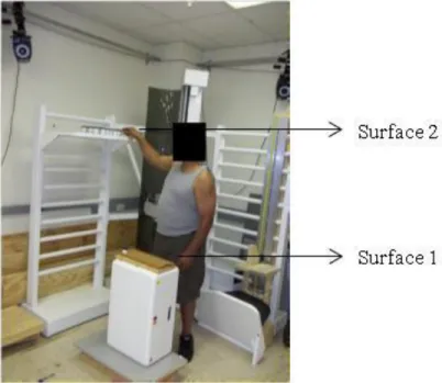
4.3.2 Custom-built manual handling workstation ... 37
4.4 Experimental tasks ... 38
vi
4.6 Experimental procedure ... 40
4.7 Data processing ... 43
4.7.1 Discrete wavelet transform (DWT) of SEMG signal ... 43
4.7.2 Wavelet function selection... 46
4.7.3 Power and power contrast calculation ... 47
4.7.4. Statistical analysis ... 48
4.7.5 Sample (participants) size determination ... 49
Chapter 5: Results ... 51
5.1 Subjective discomfort data ... 51
5.2 Right upper trapezius muscle ... 52
5.2.1 Power and frequency band trend ... 54
5.2.2 Statistical analysis ... 56
5.2.3 Comparison between the wavelet functions ... 60
5.3 Left sternocleidomastoid muscle ... 62
5.3.1 Power and frequency band trend ... 62
5.2.2 Statistical analysis ... 65
5.2.3 Comparison between the wavelet functions ... 68
Chapter 6: Discussion and Conclusions ... 70
6.1 Limitation and future works ... 73
6.2 Occupational application ... 74
6.3 Conclusions ... 74
References ... 76
Appendix A: Physical Activity Readiness Questionnaire (PAR-Q) ... 90
Appendix B: Institutional Review Board (IRB) approval form ... 91
Appendix C: Borg’s scale ... 92
Appendix D: Matlab codes for discrete wavelet transform (DWT) ... 93
Appendix E: SAS code for statistical tests ... 94
Appendix F: Participants demographic and anthropometric data ... 95
Appendix G: Exertion period ... 96
Appendix H: Individual subjective discomfort data ... 97
Appendix I: Power data (mV2) for individual participants ... 98
Appendix J: Mean (±standard deviation) of power (in mV2) calculated using ten wavelet for right upper trapezius muscle ... 108
vii
Appendix K: Output of Turkey’s test of multiple comparisons for right upper trapezius muscle ... 111 Appendix L: Mean (±standard deviation) of power (in mV2) using ten wavelet functions for left sternocleidomastoid muscle ... 126 Appendix M: Output of Turkey’s test of multiple comparisons for left sternocleidomastoid muscle... 130
viii
List of Tables
Table 4.1: Frequency bands for the seven levels of decomposition ... 43 Table 4.2: Selected wavelet functions or mother wavelets in this study ... 47 Table 4.3 : Power values for chosen number of participants... 50 Table 5.1: P-values of the Levene’s test for equality of variance of the mixed models for the
upper trapezius muscle ... 57 Table 5.2: P-values for the effect of time on the power of SEMG signal from the right upper
trapezius muscle for different wavelet functions at various frequency bands. Values marked with asterisks (*) are statistically significant... 58 Table 5.3: P-values of Tukey’s multiple comparison tests for the effect of time on the power of
SEMG signals from right upper trapezius muscle at lower frequency bands for different wavelet functions. Different times instances, T0, T20, T25 and T45 are symbolized as ‘1’,
‘2’,‘3’ and ‘4’, respectively. Values marked with asterisks (*) are statistically significant .. 59 Table 5.4: Rank and scores based on the P-values of Turkey’s multiple comparison and mixed
model for the right upper trapezius muscle. P-values of mixed model are denoted by ‘Mixed’. Different times instances, T0, T20, T25 and T45 are symbolized as ‘1’, ‘2’,‘3’ and
‘4’, respectively ... 61 Table 5.5: Power contrast (%) at the lower frequency bands: 6-12Hz, 12-23Hz and 23-46Hz for
the top 3 wavelet function for right upper trapezius muscle. Different times instances, T0,
T20, T25 and T45 are symbolized as ‘1’, ‘2’,‘3’ and ‘4’, respectively ... 62
Table 5.6: P-values of the Levene’s test for equality of variance of the mixed models for left sternocleidomastoid muscle. ... 65 Table 5.7: P-values for the effect of time on the power of SEMG signals from the left
sternocleidomastoid muscle for different wavelet functions at various frequency bands. Values marked with asterisks (*) are statistically significant ... 66 Table 5.8: P-values of Tukey’s multiple comparison tests for the effect of time on the power of
ix
different wavelet functions. Different times instances, T0, T20, T25 and T45 are symbolized as
‘1’, ‘2’,‘3’ and ‘4’, respectively. Values marked with asterisks (*) are statistically significant
... 67
Table 5.9: Rank and scores based on the P-values of Turkey’s multiple comparison and mixed model for the left sternocleidomastoid muscle. P-values of mixed model are denoted by ‘Mixed’. Different times instances, T0, T20, T25 and T45 are symbolized as ‘1’, ‘2’,‘3’ and ‘4’, respectively ... 69
Table 5.10: Power contrast (%) at the lower frequency bands: 6-12Hz, 12-23Hz and 23-46Hz for the top 3 wavelet function for left sternocleidomastoid muscle. Different times instances, T0, T20, T25 and T45 are symbolized as ‘1’, ‘2’,‘3’ and ‘4’, respectively ... 69
Table C.1: Borg’s scale of subjective discomfort rating ... 92
Table F.1: Demographic and anthropometric data of the participants ... 95
Table G.1: Task completion durations and total number of cycles for the individual participants ... 96
Table H.1: Subjective discomfort ratings ... 97
Table I.1: Power data for the 1st participant ... 98
Table I.2: Power data for the 2nd participant ... 99
Table I.3: Power data for the 3rd participant ... 100
Table I.4: Power data for the 4th participant ... 101
Table I.5: Power data for the 5th participant ... 102
Table I.6: Power data for the 6th participant ... 103
Table I.7: Power data for the 7th participant ... 104
Table I. 8: Power data for the 8th participant ... 105
Table I.9: Power data for the 9th participant ... 106
Table I.10: Power data for the 10th participant ... 107
Table J.1: Power estimated using Bior1.5 wavelet function as an effect of time for right upper trapezius muscle ... 108
Table J.2: Power estimated using Bior3.1 wavelet function as an effect of time for right upper trapezius muscle ... 108
Table J.3: Power estimated using Rbio3.1 wavelet function as an effect of time for right upper trapezius muscle ... 108
x
Table J.4: Power estimated using Coif5 wavelet function as an effect of time for right upper trapezius muscle ... 109 Table J.5: Power estimated using Db2 wavelet function as an effect of time for right upper
trapezius muscle ... 109 Table J.6: Power estimated using Db5 wavelet function as an effect of time for right upper
trapezius muscle ... 109 Table J.7: Power estimated using Db45 wavelet function as an effect of time for right upper
trapezius muscle ... 109 Table J.8: Power estimated using Haar wavelet function as an effect of time for right upper
trapezius muscle ... 110 Table J.9: Power estimated using Sym4 wavelet function as an effect of time for right upper
trapezius muscle ... 110 Table J.10: Power estimated using Sym5 wavelet function as an effect of time for right upper
trapezius muscle ... 110 Table L.1: Power estimated using Bior1.5 wavelet function as an effect of time for left
sternocleidomastoid muscle... 126 Table L.2: Power estimated using Bior3.1 wavelet function as an effect of time for left
sternocleidomastoid muscle... 126 Table L.3: Power estimated using Rbio3.1 wavelet function as an effect of time for left
sternocleidomastoid muscle... 126 Table L.4: Power estimated using Coif5 wavelet function as an effect of time for left
sternocleidomastoid muscle... 127 Table L.5: Power estimated using Db2 wavelet function as an effect of time for left
sternocleidomastoid muscle... 127 Table L.6: Power estimated using Db5 wavelet function as an effect of time for left
sternocleidomastoid muscle... 127 Table L.7: Power estimated using Db45 wavelet function as an effect of time for left
sternocleidomastoid muscle... 128 Table L.8: Power estimated using Haar wavelet function as an effect of time for left
xi
Table L.9: Power estimated using Sym4 wavelet function as an effect of time for left
sternocleidomastoid muscle... 128 Table L.10: Power estimated using Sym5 wavelet function as an effect of time for left
xii
List of Figures
Figure 2.1: Transformation of EMG signal from time domain to frequency domain using FFT.. 10
Figure 2.2: Power spectrum of a FFT transformed EMG signal ... 11
Figure 2.3: Wavelet coefficients for large- and small-scale wavelets plotted as a function of translation in time ... 16
Figure 2.4: Commonly used wavelet functions ... 17
Figure 2.5: Shrinking and dilation of a simple wavelet ... 18
Figure 2.6: Scalogram of DWT of SEMG signal using db2 wavelet function ... 19
Figure 2.7: Discrete wavelet decomposition process ... 24
Figure 2.8: Discrete wavelet reconstruction process ... 26
Figure 4.1: Telemyo 2400 G2 EMG system ... 36
Figure 4.2: Pre-amplified lead wire and snap electrode ... 36
Figure 4.3: Telemyo 2400R G2 receiver ... 36
Figure 4.4: Bipolar Ag/AgCl pre-gelled surface electrodes ... 37
Figure 4.5: Custom-built material handling workstation ... 38
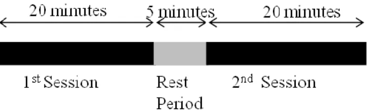
Figure 4.6: Experimental time distribution ... 39
Figure 4.7: A picture from a grocery store showing the height of the top shelves ... 40
Figure 4.8: Location of electrode on the left sternocleidomastoid muscle. ... 41
Figure 4.9: Location of electrode on the right upper Trapezius muscle. ... 42
Figure 4.10: Seven level decomposition algorithm of DWT used in this study ... 44
Figure 4.11: Reconstruction algorithm of DWT used in this study ... 45
Figure 5.1: Subjective discomfort scores at different time instances ... 52
Figure 5.2: Illustration of the raw SEMG signal and corresponding intensity pattern computed using DWT with Rbio3.1 wavelet function. Horizontal axis represents time scale in milliseconds. Blue bars separate signals collected at different time instances... 53
xiii
Figure 5.3: The graphical representation of power (mV2) as a function of time for the following wavelet functions: (a) Bior1.5, (b) Bior3.1, (c) Rbio3.1, (d) Coif5, (e) Db2, and (f) Db5 for the right upper trapezius muscle ... 55 Figure 5.4 : The graphical representation of power (mV2) as a function of time for ten wavelet
functions: (g) Db45, (h) Haar (i), Sym4, and (j) Sym5 for the right upper trapezius muscle 56 Figure 5.5: Power of SEMG signal recorded from the right upper trapezius muscle at different
time instances for the following frequency bands: (a) 6-12 Hz (b) 12-23 Hz and (c) 23-46 Hz. Behavior of Rbio3.1 and Bior3.1 wavelets were plotted using a secondary axis ... 58 Figure 5.6: The graphical representation of power (mV2) as a function of time for following
wavelet functions: (a) Bior1.5, (b) Bior3.1, (c) Rbio3.1, (d) Coif5, (e) Db2, and (f) Db5 for the left sternocleidomastoid muscle ... 63 Figure 5.7: The graphical representation of power (mV2) as a function of time for following
wavelet functions: (g) Db45, (h) Haar (i), Sym4, and (j) Sym5 for the left
sternocleidomastoid muscle... 64 Figure 5.8: Power of SEMG signal recorded from the left sternocleidomastoid muscle at different
time instances for the following frequency bands: (a) 6-12 Hz (b) 12-23 Hz and (c) 23-46 Hz. Behavior of Rbio3.1 and Bior3.1 wavelets were plotted using a secondary axis ... 66 Figure A.1: Physical Activity Readiness Questionnaire (PAR-Q) of British Columbia Ministry of Health ... 90 Figure B.1: Snap shot of Institutional Review Board (IRB) approval of this study ... 91
xiv
List of Acronyms
A (n) Approximation Vector at ‘n’ level ANOVA Analysis of Variance
Bior Biorthogonal Splines
Bior1.5 Biorthogonal wavelet function with scale of 1.5 Bior3.1 Biorthogonal wavelet function with scale of 3.1 CA Coefficients of Approximate level
CD Coefficients of Details level
cm Centimeter
Coif Coiflet
Coif5 Coiflet wavelet function with scale of 5 D (n) Detail Vector at ‘n’ level
Db Daubechies
Db2 Debauchee wavelet function with scale of 2 Db5 Debauchee wavelet function with scale of 5 Dmey Discrete Meyers
DOF Degree of Freedom
DWT Discrete Wavelet Transform EMG Electromyography
FFT Fast Fourier Transform FMF Fast Fatigable Muscle Fiber
xv Haar Haar Wavelet function
Hz Hertz
JASA Joint analysis of EMG spectrum and amplitude
Kg Kilogram
MAV Mean Absolute Value
MPD Myophosphorylase Deficiency MSD Musculoskeletal Disorders MSE Mean Squared Error
PAR-Q Physical Activity Readiness Questionnaire Rbio Reverse Biorthogonal Splines
Rbio3.1 Reverse Biorthogonal wavelet function with scale of 3.1 RMS Root Mean Square
SCM Sternocleidomastoid STD Standard Deviation
SEMG Surface Electromyography SMG Slow Fatigable Muscle Fiber STFT Short Time Fourier Transform
Sym Symlet
Sym4 Symlet Wavelet function with scale of 4 Sym5 Symlet Wavelet function with scale of 5 WMSD Work-Related Musculoskeletal Disorder WT Wavelet Transform
1
Chapter 1: Introduction
Work-related Musculoskeletal disorder (WMSD) are defined as the injuries or disorders of the muscles, nerves, tendons, joints, cartilage, or spinal discs (disorders caused by slips, trips, falls, motor vehicle accidents or similar accidents are not included) [1]. The overall impact of WMSDs is enormous in terms of individual health and corporate economics. According to U.S. Bureau of Labor Statistics [1], there were 335,390 cases of WMSDs in 2007 that accounted for 29 % of all workplace injuries requiring days away from work. The WMSDs of neck and shoulder accounted for approximately 10% of these cases [1]. In the recent data published by the Bone and Joint Decade on Neck Pain Task Force, an annual prevalence of 30% to 50% for neck pain among the general adult population was reported. Among the working population, nearly 11% to 14.1% of workers were found to suffer from disabling neck pain symptoms, i.e., they are limited in their activities because of neck pain [2]. In another study by Washington State Department of Labor and Industries, it was reported that on an annual basis more than 50,000 workers’ compensation claims were filed for WMSDs of the neck, back and upper extremity for a period between 1996 and 2004. On average, 37.5% of those claims involved WMSDs of upper extremity, neck and shoulder with an average cost of $11,334 per claim, costing approximately $3.8 billion in direct costs. [3].
Different types of physical exertion were deemed to be the causal factors of work-related neck and shoulder pain in the epidemiological studies. Physical exertions that demand low levels of prolonged and/or repetitive movement are associated with inflammatory-type neck pain syndromes such as trapezius myalgia, cervicalgia, etc. [4]. Whereas forceful arm exertion required in physically demanding activities are identified as the risk factors for disc specific
2
diseases, such as herniated/protruded discs. In the recent years, evidence for a causal relationship between work-activities that demand sustained, sub-maximal repetitive exertions and neck and shoulder WMSDs is mounting in the literature [2, 5-7]. Such exertions performed over sustained period of time cause overuse of muscles, nerve, and joints leading to neuromuscular fatigue, which is believed to be the precursor of WMSDs. Therefore, quantitative assessment of muscle fatigue is essential for early detection and prevention of risks of WMSD [8]. An accurate assessment of fatigue caused by different types of exertions could also facilitate development of intervention strategies to mitigate risks of WMSDs.
There are a number of techniques that can be used for the objective assessment of fatigue. Some of these techniques/methods involve measurement of maximum voluntary contraction, endurance time, power output, etc. A few studies have also used subjective methods such as measurement of perceived effort, discomfort ratings, etc. for the evaluation of fatigue. Most of these methods are more sensitive to the changes that are more representative of fatigue caused by high force or static sustained exertions and are not receptive to the subtle physiological changes caused by the sub-maximal repetitive exertions. Surface electromyography (SEMG) is a non-invasive and fairly accurate tool for continuous monitoring of muscle fatigue during a physical activity [9-11]. Most popular method used for evaluating muscle fatigue using SEMG is the study of median frequency pattern. A drop in the median frequency is known as the one of the biomarkers of muscle fatigue. Calculation of median frequency is based on the Fast Fourier Transform (FFT), which identifies frequency content of a signal but is unable to determine when a particular frequency component of the signal takes place in time. For a stationary signal (all frequency components exist at all times) timing information is irrelevant and shift in the power spectrum frequencies provide valuable information about the muscle fatigue. Isometric constant
3
force contraction was treated as a stationary signal for fatigue assessment using FFT in previous studies [12]. However, under dynamic conditions the surface electromyography signal is non-stationary and fatigue assessment using FFT may not provide accurate assessment [7, 9, 13]. Short Term Fourier Transform (STFT) provides a possible solution to this problem [12], however it cannot solve time and frequency resolution issues. A short window size in STFT provides better time resolution, but poor frequency resolution; while a relatively long window provides better frequency resolution but poor time resolution [12].
The Discrete Wavelet Transform (DWT) analysis provides a potential solution to this dilemma of resolution and is becoming a more common digital signal processing method for analyzing SEMG signals. It acts as a “mathematical microscope” in which one can observe different parts of the signal by just adjusting the focus. This allows the detection of short-lived time components of signals. Another advantage of DWT is the availability of various orthogonal wavelet functions that allow the most appropriate to be chosen for the signal under investigation [14]. In recent years although a number of researchers have used DWT for evaluating muscle fatigue using surface electromyography [13-19], its application to neck and shoulder muscle fatigue is not well established. In this study, DWT analysis was established as a suitable method to conduct quantitative assessment of neck and shoulder muscle fatigue caused by repetitive exertions.
4
Chapter 2: Literature Review
2.1 Neuromuscular fatigue and WMSD
The major risk factors that are typically associated with the WMSDs of neck and shoulder include genetic, morphological, psychosocial, and biomechanical factors [20]. Among these factors, genetic and morphological factors play important role in understanding the prevalence of WMSDs. The biomechanical factors are critical in determining effective control strategies. Biomechanical factors that are most frequently associated with WMSDs of neck and shoulder includes work activities that demands low levels of prolonged exertions, repetitive arm exertions, or forceful arm exertions. Exertions that demand low levels of prolonged and/or repetitive exertions are frequently performed by office workers, sewing machine operators, dental hygienists, and surgeons [21-26]. Whereas forceful arm exertions are commonly performed by the workers in occupations such as health care, construction work, farm work, and manual material handling industries [27-32]. Low levels of sustained exertions and/or sub maximal repetitive exertions were typically associated with inflammatory-type neck pain syndromes such as trapezius myalgia, cervicalgia, etc. [4]. Whereas heavy exertions are identified as the risk factors for the disorders such as tension neck syndrome and disc specific diseases such as herniated/protruded discs.
In the recent years, the incidence rate of inflammatory-type neck and shoulder pain syndromes among working population in the USA has shown an increasing trend [2, 5-6]. Overuse of muscles, nerves, and/or joints caused by repetitive movements leads to muscle fatigue which is believed to be the precursor of most of the inflammatory-type neck and shoulder
5
musculoskeletal disorders. Therefore, quantitative assessment of muscle fatigue is essential for early detection and prevention of risks of WMSDs [8]. An accurate assessment of fatigue caused by different types of exertions could also facilitate development of intervention strategies to mitigate risks of WMSDs. In an early fatigue study, Rohmert [33] stated that static contractions performed above 30% of maximal voluntary contraction (MVC) may result in early fatigue increasing the risk of WMSDs. He suggested that static contractions below this level represent a safe limit for muscle load and may reduce risk of WMSDs.
Chaffin [34] performed a study to evaluate postural risk factors for WMSDs of the neck using subjective and objective assessments of muscular fatigue. He found that tilting the head/neck forward more than 30º greatly increases the neck extensor fatigue and recommended work-place design changes such that the tilting angle can be reduced to 15º or less to prevent fatigue and, subsequently, the risk of neck WMSDs. In a study of fish processing workers in Taiwan, Chiang et al., [35] studied the relationship between workplace factors and shoulder girdle pain using fatigue estimates. Shoulder girdle pain was defined as self-assessed symptoms of pain in the neck, shoulder or upper arms, and signs of muscle tender points or palpable hardenings upon physical examination. Fatigue caused by different types of exposure outcomes in terms of force and repetitiveness was evaluated using surface electromyography. Using multiple logistic regression analysis with age, gender, and force as co-variants, the authors determined that highly repetitive upper extremity movements generated fatigue that was associated with shoulder girdle pain.
Neuromuscular fatigue has also been used by a number of scientific committees to setup workplace guidelines. In a report published by National Research Council in 1999 it was stated that “Scientists with experience of policy setting affirmed their belief that it was prudent to
6
consider fatigue as a potential precursor to some of the disorders under consideration” [36]. In the Annex of Council Directive set up by the European Directives and Standard to establish safety and health requirements for the computer users in recognition of the importance of fatigue with respect to keyboard use, it was stated that: "(c) Keyboard: The keyboard shall be tilt-able and separate from the screen so as to allow the worker to find a comfortable working position avoiding fatigue in the arms or hands” [37]. In the European WMSD standards on Machinery Directive (prEN 1005-3) estimates of force limits for machinery operation were primarily derived on the basis of decreasing fatigue during work to reduce WMSDs [37].
2.2 Quantification of fatigue
In ergonomics literature, the terms muscle fatigue and neuromuscular fatigue have been used interchangeably [34]. Muscle Fatigue has generally been defined as an acute impairment of mental or physical performance as a result of an increase in the perceived effort necessary to exert force, regardless of whether a subject can still perform the task successfully or not [38-39]. Vollestad [40] defined neuromuscular fatigue as the reduction of force generating capacity of the muscular system, usually seen as a failure to maintain or develop a certain expected force or power. In the scientific literature, researchers have used the following five assessment methods to quantify neuromuscular fatigue.
1) Changes in the Maximum Voluntary Contraction (MVC): MVCs are executed by instructing the participants to produce the highest possible force, in a setting where the length changes are restricted to the initial tightening up of the muscle-tendon unit (isometric exertion). The changes in recorded force before and after a bout of exertions are used to estimate muscle fatigue. A significant decrease in the force exertion during the MVC contraction indicates the sign of fatigue. In a study, Newham et al., [41] examined the force generating capacity
7
during the MVC exertions before and after 4 min of knee extension activities. Authors observed 80% decreases in the force exertion during the MVC exertions after 4 minutes of knee extension activities.
2) Changes in the endurance time: In many studies, fatigability is examined by assessing the endurance time. This approach is based on a presumption that there is an association between the decline in maximal force generating capacity and the time to exhaustion. Garg et al., [42] studied the fatigue of shoulder girdle musculature by using isometric contraction performed at different shoulder postures under different weight conditions. The weights used by the participants were 5%, 15%, 30%, 45%, 60%, 75%, and 90% of the MVC at each of the shoulder postures. With an increase in the weight, the endurance time decreased significantly. The decrease in endurance time followed a non-linear trend and corresponded very well with the subjective assessment measures of fatigue and pain ratings.
3) Changes in the metabolite concentration: There are a number of metabolic changes that occur concurrently with muscular fatigue. The relationship between intracellular metabolites and the force exertion during fatigue has been examined in a number of studies [43-45]. Most of these studies indicated that the normal participant’s intracellular pH value decreases as the muscle is fatigued. Cady et al., [44] studied the first dorsal interosseous muscle of the hand by fatiguing the muscle with three bouts of maximal voluntary contraction. The intracellular phosphorus metabolites were measured by nuclear magnetic resonance during the intervals between the fatiguing contractions. The relationships between loss of force and change in metabolite concentrations were obtained from four normal participants and one subject with myophosphorylase deficiency (MPD) who could not utilize muscle glycogen and therefore produced no hydrogen ion from glycolysis. For both the MPD and normal participants the
8
relationship between relative force loss and inorganic phosphate concentration was found to be curvilinear.
4) Near-infrared spectroscopy: This technique utilizes oxygenation properties of skeletal muscle to estimate muscle fatigue [46]. A muscle shows significant changes in the hemoglobin oxygenation and blood volume during fatiguing contracting [46-48]. Yoshitake et al., [47] used near-infrared spectroscopy to investigate the etiology of lower-back fatigue. They compared isometric back extensions for a period of 60 seconds performed at an angle of 15° with 0° horizontal plane. It was observed that oxygenation and the blood volume of the lower back muscles decreased significantly throughout the exertions performed at 15° compared to those performed at 0°.
5) Electromyography (EMG): This is probably one of the most widely used methods in fatigue quantification in the occupational settings. EMG has been extensively used to study the patterns of activation or tension developed in the muscles during a variety of occupational tasks. There are two types of EMG data recording techniques: intramuscular EMG (needle of fine-wire) and surface EMG (SEMG). Intramuscular EMG involves inserting needle or fine-wire electrodes directly into the muscle through the skin and is invasive in nature. In SEMG, surface electrodes are placed on the muscle of interest over the skin to record the muscle activity [49]. Surface electrodes pick up changes in the muscle activation resulting from either a changed number of active muscle fibers or excitation rates [50]. Electrical activity picked up by the surface electrodes reflects a summary of active motor unit action potential, which reflects a chemical- electrical process in several muscles’ fibers and motor units [51]. The EMG data can be processed using time domain or frequency domain analysis. Time domain analysis typically deals with amplitude estimation, while frequency domain
9
analysis deals with the trends in the different frequencies in the signal. The following methods are commonly used by the researchers to evaluate EMG signal for the objective assessments of fatigue:
I. Change in the EMG amplitude: There are two methods that are most commonly used to estimate changes in the amplitude of the EMG signal: mean absolute value (MAV) [52] and root-mean-square (RMS) value [53]. The equations used for computation of these values are as follows [54]:
(2.1)
(2.2)
Where,
Xi is the ith sample of the signal
N number of samples in the signal
In previous studies, it was shown that EMG amplitude increases with fatigue due to additional recruitment of motor units during the exertions that are physically demanding, such as maximal or near maximal exertions [55-56].
II. Change in the Zero-crossing rate (ZCR) of the signal: Zero-crossing rate (ZCR) is defined as half the number of zero crossing of EMG signal (S(t)) per second [57]. If both the first derivative S0(t) and signal S(t) have a Gaussian amplitude, the distribution
of the expected zero-crossing rate Z can be calculated as [58] –
10
Where, S (f) is the Power Spectral Density (PSD) of the signal and fs is the sampling
frequency. Inbar et al., [57] showed that the ZCR can be used to monitor the spectral changes of EMG signal. Authors observed that zero crossing of the raw EMG signal shifts to lower values as an indicator of muscle fatigue.
III. Changes in the frequency spectrum variables: To estimate changes in the frequency content of the EMG signal, the raw EMG signal is transformed from the time domain to the frequency domain (Figure 2.1). Fast Fourier transform (FFT) is the most frequently used method for conducting this transformation. By using FFT, the frequency spectrum of EMG signals are clarified and recognized by breaking down the signal into its corresponding sinusoidal of different frequencies [59]. Three variables based on the FFT transformed data that are often used to estimate muscle fatigue are (Figure 2.2):
Figure 2.1: Transformation of EMG signal from time domain to frequency domain using FFT (1) Mean frequency: the mathematical mean of the spectrum curve
(2) Median frequency: the parameter that divides the total power area into two equal parts
(3) Total power: The integral of the spectrum curve (Figure 2.2).
Fast
Fourier
Transform
(FFT)
11
Figure 2.2: Power spectrum of a FFT transformed EMG signal
A number of previous studies have used changes in the median frequencies of EMG data to evaluate muscle fatigue [56]. A shift in the median frequencies to lower values has been identified as the indicator of neuromuscular fatigue in most of these studies. For example, in a study conducted by Potvin et al., [56] behavior of the bicep brachii muscle was evaluated using changes in the median frequencies of the EMG signal during fatiguing contractions. The authors found that muscle fatigue resulted in the drop of median frequencies. In another study by Georgakis et al., [60] fatiguing behavior of knee extensors was studied during the isometric knee extension. A consistent decrease in the median frequencies of knee extensor muscles, vastus medialis, vastus lateralis, and rectus femoris muscles, was reported by the authors. A drop in the mean frequency has also been used as the biomarker of fatigue in a few studies. However, a relatively lower coefficient of variation for the mean frequency was reported than the median frequency. In terms of power, an increase in the power of the low frequency components of the EMG and a decrease in the power of high frequency components were reported by a number of authors for various muscles in the human body with the onset of fatigue [50, 56, 59, 61-62].
12
IV. Joint analysis of EMG spectrum and amplitude (JASA): In non-isometric contractions, sometimes it is very difficult to interpret changes in the spectrum and amplitude of the surface EMG signal independently [54]. At such instances, simultaneous consideration of amplitude and spectrum related variables of EMG signal is essential to provide information on whether EMG changes are fatigue-induced or force-related. JASA uses the following four criteria to distinguish fatigue-induced or force-related changes caused by a dynamic exertion [63]:
(1) If the EMG amplitude increases and EMG spectrum shifts to the right, muscle force increase is the probable cause.
[37](2) If the EMG amplitude decreases and EMG spectrum shifts to the left, muscle force decrease is the probable cause
(3) If the EMG amplitude increases and EMG spectrum shifts to the left, this is considered to be result of muscle fatigue
(4) If the EMG amplitude decreases and the EMG spectrum shift to the right, this is considered to be recovery from previous muscle fatigue.
V. Short-time Fourier transform: Isometric muscle contractions can be easily analyzed for muscle fatigue by using either of the above mentioned time or frequency domain analysis method. Evaluation of fatigue caused by dynamic contraction is rather problematic because of its time variant nature. For such signal, variations of the EMG signal spectrum cannot be analyzed by simply applying Fourier transform, since information about time would be lost. Also, generally speaking, EMG signals do not conform to the stationary requirement of the Fourier transform. One way to satisfy this requirement is to apply Fourier transform only to signal segments that are short enough
13
to fulfill this requirement. Short-time Fourier transform (STFT) provides the potential solution to this problem, where the EMG signal is divided into short time windows and Fourier transform is applied to each window. STFT also provides an insight into variations of the spectrum as a function of time. It is defined as [12]
(2.4)
Where f is the sinusoidal frequency, t is the time and w is the normalized window. STFT analyzes the signal x(t) through a short-time window w(t): x(t)w(t-τ ), and then a Fourier transform is performed on this product. Previously, STFT was used by Sparto et al., [64] to study fatigue of low back muscles caused by isokinetic exertions. The authors used a window size of 1 second to compute the Fourier transform. A significant decline in the median frequency was reported by the authors in this study.
2.3 Shortcoming of EMG data analysis methods
Amplitude analysis in time domain is a simple data reduction technique of an EMG signal that provides a crude estimation of the exposure level. However this method does not provide detailed information regarding exposure dynamics. Amplitude increases with force as well as fatigue, so it is difficult to interpret whether the amplitude modification represents a fatigue or force change [63]. Moreover, in the presence of additive noise, amplitude based methods are subjected to overestimation errors [65]. ZCR provide a reliable estimate of spectral changes, but it is highly dependent on signal-to-noise ratio (SNR) of the analyzed EMG signal. Moreover, ZCR is also very sensitive to the deviations of the amplitude distribution from Gaussian one [66-67]. The JASA considers simultaneous discrimination between fatigue-induced
14
and force-related changes with time in the EMG signal [63, 68]. The dependencies of spectral variables on force can neither be fully explained nor be clearly understood, hence it is questionable to reach a precise conclusion of muscle fatigue based on the four possible case algorithm presented by JASA during non-isometric contractions [68].
Algorithms based on the Fourier transform (FT) are the most widely used methods to describe the spectral content (power spectral density (PSD) of EMG signal [69]. FFT based analyses identify frequency content of a signal but do not determine when a particular frequency component of the signal takes place in time. For a stationary signal (all frequency components exist at all times) timing information is irrelevant and shift in the power spectrum frequencies provide valuable information about the muscle fatigue. In the real world, force level and body posture do not remain constant during physical activities. During such exertions, the level of force application changes continuously. The SEMG signal recorded during such exertions is non-stationary in nature i.e. all frequency components are not present at all the times. [62]. The FFT analysis of such non-stationary signals could only provide spectral information of different frequencies without providing sufficient information regarding when a particular frequency content of the signal takes place in time [70].
Short-Time Fourier Transform (STFT) provides a possible solution to this problem, however, it presents time and frequency resolution issues [12]. A short window size in STFT provides better time resolution, but poor frequency resolution and relatively longer window provides better frequency resolution but poor time resolution. In some applications this can be a rather irrelevant, yet in others it may be a limitation. For example, if the analyzed signal is a mixture of short-duration high-frequency events that are closely spaced in time and long-duration low frequency components that are closely spaced in frequency, STFT cannot provide
15
appropriate time resolution for distinguishing high-frequency events along with adequate frequency resolution for distinguishing low frequency components [54, 67].
The wavelet transform (WT) analysis provide a potential solution to this dilemma of resolution and is becoming a more common digital signal processing method for analyzing EMG signals. Discrete Wavelet Transform (DWT) acts as a bank of low-pass and high-pass filters that decompose a signal into multiple signal bands. It separates and retains the signal features in one or a few sub-bands and presents a method for analyzing the temporal occurrence of frequency alterations in a signal [71]. In the following section a detailed description of how wavelet transforms works is provided.
2.4 Wavelet transform
Just as STFT is based on a family of sinusoids used to decompose EMG signal within successive windows of time, wavelet transform (WT) implements a set of time scaled and time translated versions of a basic wavelet function. Just as the original signal can be built back up from its Fourier components by adding those components all together in the right proportions and with the right phase lags, the original waveform can be built back up from its wavelet components by adding those wavelet components all up in the correct proportions and with the correct time translations. Computationally, the WT uses wavelets to break down EMG signal in much the same way that the STFT uses windowed sine and cosine waves. Figure 2.3 provides a simplified illustration of the WT of an EMG signal for two of the many possible different scales of waveform structure, a large scale and a small scale. At the large scale, the wavelet is aligned with the beginning of the neuroelectric waveform and the correlation of the wavelet shape with the shape of the neuroelectric waveform at that position is computed. This correlation, known as a wavelet coefficient, measures how much of the wavelet at that scale and position is included in
16
the neuroelectric waveform. The same wavelet is then translated (moved) a small amount to a later position in time, bringing a slightly different portion of the neuroelectric waveform into the ‘‘view’’ of the wavelet and a new wavelet coefficient is computed. This process continues until all possible translations of the wavelet at the large scale have been exhausted and their corresponding wavelet coefficients have been computed [71].
Figure 2.3: Wavelet coefficients for large- and small-scale wavelets plotted as a function of translation in time [77]
The coefficient plot at the bottom of Figure 2.3 illustrates the wavelet coefficients that correspond to each position of the large-scale wavelet as it moves along the signal in time. The large-scale wavelet is frozen in time at a position where it closely correlates with the local shape of the signal. Generally, whenever the wavelet shape matches the overall shape of the signal, a large wavelet coefficient is computed, with positive amplitude if the match is normal and negative amplitude if the match has inverted polarity. Conversely, when the shape match is poor, a small or zero wavelet coefficients is computed. Hence, the core of a wavelet transform is the
17
appropriate selection of the mother wavelet. It is this wavelet that is used to form the first and subsequent detail functions. If the mother wavelet shape is better matched with the EMG waveform, it can localize high time and frequency information [72-73].
Figure 2.4: Commonly used wavelet functions[71]
Mother wavelets with wide variety of shapes are available for conducting WT. Some commonly used wavelet functions, like the Haar, Daubechies, and Coifman 30 wavelet functions are shown in Figure 2.4. Wavelet functions can be scaled in time by stretching or shrinking them and can be moved (translated) to different time positions at any scale without changing their basic shape. Scaling and translation are the two basic parameters of wavelet representations. Higher scale is proportional to lower frequency and higher frequency is proportional to lower scale. The set of all scaled and translated wavelets of the same basic wavelet shape forms a wavelet family. There are an infinite number of wavelet functions in a wavelet family because there are, in principle, an infinite number of scales and an infinite number of time translations for any wavelet [71-74]. Stretching a wavelet to a larger scale makes it less localized in time (more
18
spread out), and its spectrum (Figure 2.5) consequently shifts to lower frequencies and concentrates more over a smaller bandwidth. That is, it becomes more localized in frequency. Conversely, shrinking a wavelet to a smaller scale makes it more localized in time, and its spectrum shifts to higher frequencies and spreads out more over a larger bandwidth. That is, it becomes less localized in frequency.
Figure 2.5: Shrinking and dilation of a simple wavelet[77]
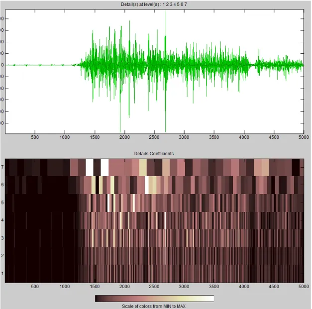
Figure 2.6 shows a DWT transform of a signal into seven decomposition levels and how each level (scales) has both localized corresponding time and localized frequency information. The bright (minimum to maximum) spots represent the highest localized content of those frequency band (scales) in that particular time period [73]. Thus, wavelets obey a fundamental uncertainty principle, the Heisenberg Uncertainty Principle, which states that time localization trades off against frequency localization as wavelets are stretched or shrunk.
19
Figure 2.6: Scalogram of DWT of SEMG signal using db2 wavelet function
2.5 Wavelet family
The mother wavelet produces all wavelet functions used in the transformation through translation and scaling and therefore it determines the characteristics of the resulting wavelet transform. The wavelet functions are chosen based on their shape and their ability to process the signal in a particular application [17]. The following orthogonal mother wavelets are available for conducting wavelet transform [73]:
20
1) Haar wavelet family: This is the oldest and the simplest wavelet family. Its filter has only one vanishing moment, perfect reconstruction and aliasing cancelation capability. With a basic filter length of only 2 points it has excellent time resolution but poor frequency resolution. Generally Haar wavelet families are good for edge detection, for matching binary pulses, and for very short phenomenon [73].
2) Daubechies wavelet family: These wavelet functions (filters) are robust, fast, and adaptable. They are in wide use for identifying signals with both time and frequency characteristics. Being non-symmetric, Daubechies wavelet functions may be passed by in favor of some symmetric wavelets for image processing because the human eye is more tolerant of symmetric errors [73].
3) Symlet wavelet family: Symlet wavelet family is compactly supported wavelets with the least asymmetry and highest number of vanishing moments for a given support width. It is more symmetrical than the Daubechies. Being nearly symmetrical, the larger Symlet function (Sym 12, Sym16, etc.) also have a nearly linear phase. Other than the symmetry and phase, Symlets share the same properties as the Daubechies wavelet family. They become more regular with larger N (“SymN"). They have the same compact support as the Daubechies for a given N, they have the same number of vanishing moments as the DbN family, and they have the perfect reconstruction and alias cancellation capability [73]. 4) Coiflet wavelet family: Coiflet wavelet family is compactly supported wavelet function
with the highest number of vanishing moments for both phi and psi for a given support width. It was developed by Ingrid Daubechies at the request of wavelets pioneer Ronald Coifman to invent an orthogonal wavelet (filter set) that had vanishing moment capabilities for both the high pass and low pass filters. These Coiflet wavelet function have the same
21
orthogonality relationships as the Daubechies Wavelets and the Symlet filters and also possesses alias cancellation and perfect reconstruction capabilities [73].
5) Discrete Meyer wavelet family: The continuous Meyer Wavelet is originated in the frequency domain, which produce excellent frequency characteristics. The discrete Meyer wavelet functions satisfy the orthogonality conditions and they also have perfect reconstruction capability. These wavelets do not have vanishing moments; however, they have nearly perfect symmetry and linear phase [73].
6) Biorthogonal wavelet family: BioSpline or Biorthogonal wavelet functions have vanishing moments and perfect reconstructions capability. The most useful property of it is symmetry with FIR filters, while the main difficulty is its lost orthogonality. Biorthogonal Wavelets are in wide use in image processing because of their perfect symmetry. Image compression and denoising can be accomplished efficiently using the biorthogonal filters [73].
7) Reverse Biorthogonal wavelet family: These are compactly supported biorthogonal spline wavelet functions with symmetry and perfect reconstruction capability [73].
2.6 Discrete Wavelet Transform (DWT)
Most of the time, signals are sampled at discrete time points with limited resolution and one must use a very limited number of discrete incremental scales and time translations if they are going to produce an answer in a reasonable amount of time. The discrete wavelet transform (DWT) technique was introduced by Mallat [72]. The DWT provides highly efficient wavelet representation that can be implemented with a simple recursive filter scheme, but provides no redundancy. Moreover, it only produces as many coefficients as there are sampled within the original signal, without the loss of any information at all. Consequently, the DWT permits
22
perfect reconstruction of the original waveform by an inverse filtering operation. In general, the discrete wavelet tools have capabilities for both signal analysis and signal processing, such as noise reduction, data compression, peak detection and so on [71]. A number of studies employed discrete wavelet transform to study Electromyography signal [13-19].
The DWT coefficients are usually sampled on a dyadic grid. Given that the signal is a discrete time function and interchangeable sequence is denoted by X[n], where n is an integer. The DWT is computed by successive low pass and high pass filtering of the discrete time domain signal. First of all, the signal (sequence) will pass through a half band digital low pass filter with impulse response P[n] and filter the signal by convoluting the signal with the impulse response of the filter. The convolution operation in discrete time is defined as follows [17]:
(2.5)
To understand the DWT it is necessary to understand a remarkable property of wavelets. It is possible for wavelets to be orthogonal, meaning that a subset of a given wavelet family can be chosen from specially selected scales and translations in such a way that none of the scaled and translated wavelets in the subset correlate with each other at all. Such subsets are said to form an orthogonal basis for representing real functions. That is, any EMG waveform can be perfectly constructed by adding together point-for-point in time all of the orthogonal wavelets in the subset after correctly setting their individual magnitudes. Hence, the DWT algorithm consists of two phases, the decomposition phase and the reconstruction phase. In 1988, Mallat produced a fast wavelet decomposition and reconstruction algorithm [72].
23 2.6.1 Discrete wavelet decomposition
The DWT analyzes the signal at different frequency bands with different resolutions by decomposing the signal into a coarse approximation and detail information. DWT employs two sets of functions, called scaling functions and wavelet functions, which are associated with low pass and high pass filters, respectively. The procedure of decomposition starts with passing the signal X [n] through a series of half band high pass filters H[n] to analyze the high frequencies, and passing through a series of half band low pass L[n] filters to analyze the low frequencies. The coefficients resulting from the high pass filter band are known as ‘details coefficients’ and the coefficients found in low pass filter band are known as ‘approximate coefficients’. To obtain additional scales of waveform information, the first detail function is set aside and the approximate coefficients for the low resolution signal after the first filtering operation are fed back through the two filters simultaneously, giving a second set of small-scale wavelet coefficients and a new set of coefficients for the low resolution signal. This procedure can mathematically be expressed as
(2.6)
(2.7)
In equation (2.6) and (2.7), Y high[k] and Y low[k] are the outputs of the high pass and low
pass filters respectively, after down sampling by 2. The above procedure, known as the sub band coding, can be repeated for further decomposition. At every level, the filtering and sub sampling will result in half the number of samples (and hence half the time resolution) and half the frequency band spanned (and hence doubles the frequency resolution) [17, 71].
24
To illustrate with an example, it is assumed that the signals have ‘n’ points and ‘f’ highest frequency and run through high pass filter, and low pass filter, whose filter coefficients are uniquely determined by the particular wavelet shape that is to be used in the analysis. Different wavelet shapes are associated with different filter coefficient sequences. The filtering operation can eliminate half of the samples according to Nyquist’s rule. The output of each filter is a series of n wavelet coefficients. Every other coefficient is discarded from the series, leaving n/2 coefficients for each filter output. This process of discarding alternate coefficients is known as down sampling and is indicated by the downward pointing arrow and adjacent ‘‘2’’ symbol (Figure 2.7). The signal now has a highest frequency of f /2 radians instead of f. The low pass filter output captures all of the low frequency energy of the waveform (0 – f/2) and the high pass filter output captures all of the high frequency energy of the waveform (f/2 – f). This constitutes one level of decomposition.
Figure 2.7: Discrete wavelet decomposition process [77]
This signal is then passed through the same low pass and high pass filters for further decomposition. This process continues until two samples are left. The maximum level of
25
decomposition depends on the signal length. If the signal has ‘N’ number of data points, the maximum level of decomposition will be
Q = (2.8)
Equation (2.8) can also be expressed as – N = .
The maximum level of decomposition is also known as full decomposition. A neuro-electric signal can be decomposed at any level within the maximum level of decomposition, depending on the choice of frequency bands. Each of these wavelet levels correspond to a frequency band. The maximum frequency that can be measured is given by the Nyquist theory as
(2.9)
is the maximum frequency band of the signal if the sampling frequency of the signal is [75].
In Figure 2.7, each successive detail function– D1, D2, D3, … D (n) and approximate function – A1, A2, A3,… A (n) has a spectrum with a center frequency ( f ) and bandwidth ( ∆f ) that is half those of the previous detail function and approximate function. As an example, the frequency of the first level details is and the frequency of the first level approximation is . Thus, frequency resolution improves by a factor of 2 for each successively larger scale in a DWT while time resolution correspondingly decreases by a factor of 2. Conversely, time resolution improves by a factor of 2 at successively smaller scales and frequency resolution correspondingly decreases by a factor of 2. The corresponding frequency band of each level will appear as high amplitudes in that region if these are prominent frequencies in the original signal. On the contrary, the frequency bands that are not very
26
prominent in the original signal will have very low amplitudes, and that part of the DWT signal can be discarded without any major loss of information.
2.6.2 Discrete wavelet reconstruction
Since the wavelet transform is a band pass filter with a known response function (the wavelet function), it is possible to reconstruct the original time series using either deconvolution or the inverse filter. This is straight-forward for the orthogonal wavelet transform (which has an orthogonal basis), but for the continuous wavelet transform it is complicated by the redundancy in time and scale. The original EMG signal can be built back up from its wavelet components by adding those wavelet components all up in the correct proportions and with the correct time translations [76-77]. The signal reconstruction procedure follows the reverse order of the signal decomposition. Figure 2.8 represents the schematic diagram of the signal reconstruction where the signals at every level are up-sampled by two, and passed through the synthesis filters L/[n], and H/[n] (low pass and high pass, respectively), and then added.
27
Both the analysis and synthesis filters are identical to each other, except for a time reversal. Therefore, the reconstruction formula for each level can be written as
(2.10)
Regardless of the number of detail functions generated, the total number of wavelet and scaling function coefficients necessary to exactly reconstruct the original waveform always equals the number of original waveform samples. However, if the filters are not ideal half band, then perfect reconstruction cannot be achieved. Although it is not possible to realize ideal filters, under certain conditions it is possible to find filters that provide perfect reconstruction. Hence, the best wavelet function selection is a very crucial issue in DWT analysis [77].
2.7 Previous studies of DWT and neuromuscular fatigue
2.7.1 DWT as a better tool for neuromuscular fatigue determination
Discrete wavelet transform in SEMG signal analysis lays a foundation for studying the muscle fatigue in a variety of muscle contraction modes. The quantification of the amount of neuromuscular fatigue of the back during repetitive exertions has been performed by using DWT in SEMG signal processing. For this purpose, Sparto et al., [64] used filter banks and wavelets to determine additional insights into the fatigue process during repetitive isokinetic trunk extension tasks. They also decided which measures were more highly correlated with the decline in maximal trunk extension torque. Trunk muscle electromyograms were collected from 16 healthy men performing repetitive isokinetic trunk extension endurance tests over a four week period. The test was controlled at 35% and 70% of the participants’ maximal voluntary contraction while they exerted at 5 and 10 repetitions per minute to induce different rates of fatigue. SEMG data were analyzed using the wavelet and the traditional Short Time Fourier methods. Linear
28
regression quantified the rate of change in Fourier and wavelet measures caused by fatigue, whereas Pearson’s correlation coefficient determined their association with the decline in maximum torque. Six scales of Daubechies wavelet were selected that resulted in adequate coverage of the frequency range expected for SEMG signals (i.e., 5–300 Hz). Wavelet coefficients were computed for each wavelet function and scale during each exertion. The root-mean-square value was calculated for the 1 second of data corresponding to the trunk range of motion between 25° and 10°. RMS torque in the STFT and wavelet measures were quantified using simple linear regression. The statistical analysis of regression reflected that repetition rate is a significant factor that affects the decline in maximal torque. There was a significant decrease in the scale 4 coefficients (209–349 Hz) and a significant increase in scale 32 coefficients (26–44 Hz) and scale 64 coefficients (13-22 Hz) for 10 repetitions. Only 69% of the coefficients at the same scale were significantly increased during the trials of 5 repetitions per minute. The same trends were also observed during STFT. In addition, the decline in maximal torque output was significantly affected by exertion magnitude. The correlations between the rate of change in the RMS value of Daubechies wavelet coefficient and the maximum torque output decline were positive for scale 4 (the high-frequency range) and negative for the other scales. Hence they showed that DWT is a validated tool for quantifying and detecting back muscle fatigue.
The most commonly used parameters describing the spectral content of SEMG, such as Fourier-based mean and median power frequencies, are routinely used to characterize muscle activity and fatigue in many physiologic and pathologic circumstances. The application of the Fourier transform to a data stream is only limited for stationary signal, but for the cases where repetitive or non-constant muscular activity is considered, stationary constraints are violated.
29
Hence the researchers proposed the use of multi-resolution wavelet analysis which provides both temporal and frequency resolution of a signal [78]. In order to determine the ability of this method, T. Vukova [79] investigated fatigue-induced changes in the spectral parameters of slow (SMF) and fast fatigable muscle fiber (FMF) action potentials using DWT and FFT. Intracellular potentials were recorded during repetitive stimulation of isolated muscle fibers immersed in Ca2+-enriched medium, while extracellular potentials were obtained from muscle fibers pre-exposed to electromagnetic microwaves. The changes in the frequency distribution of the action potentials during the period of uninterrupted fiber activity were used as criteria for fatigue assessment. The results showed a fatigue-induced decrease of potential high frequencies (SMF: 59% vs. 96%, MMW vs. control; FMF: 30% vs. 92%, respectively), and an increase of low frequencies (SMF: 200% vs. 207%, MMW vs. control; FMF: 93% vs. 314%, respectively). They further observed that DWT provides a reliable method for estimation of muscle fatigue onset and progression from data analysis of RMS analysis of the wavelet coefficients.
The frequency characteristics of random signals like SEMG can be studied by power spectrum analysis by using wavelet transform function. Changes in the SEMG power spectrum are used as an indicator of changes in muscle contraction and muscle fatigue for ergonomic purposes [80]. These SEMG power spectrums are also varied when different wavelet functions are used and it is not clear which wavelet function offer appropriate results. In a gait analysis using various wavelet functions, Reaz and Hussain [81] analyzed SEMG power spectral parameters and compared different wavelet families. In this research, SEMG were decomposed using Discrete Wavelet Transform (DWT) with various wavelet families (WFs) - Haar, Daubechies (db2, db3, db4, db5, db45) and Symlet (sym4, sym5) at Matlab environment. The authors collected 11 separate EMG data files for the 9 trial walks, muscle at rest level, and

![Figure 2.3: Wavelet coefficients for large- and small-scale wavelets plotted as a function of translation in time [77]](https://thumb-us.123doks.com/thumbv2/123dok_us/1444635.2693379/32.918.107.499.309.707/figure-wavelet-coefficients-large-wavelets-plotted-function-translation.webp)
![Figure 2.4: Commonly used wavelet functions [71]](https://thumb-us.123doks.com/thumbv2/123dok_us/1444635.2693379/33.918.109.291.276.596/figure-commonly-used-wavelet-functions.webp)
![Figure 2.5: Shrinking and dilation of a simple wavelet [77]](https://thumb-us.123doks.com/thumbv2/123dok_us/1444635.2693379/34.918.112.633.317.601/figure-shrinking-dilation-simple-wavelet.webp)
![Figure 2.7: Discrete wavelet decomposition process [77]](https://thumb-us.123doks.com/thumbv2/123dok_us/1444635.2693379/40.918.121.746.469.956/figure-discrete-wavelet-decomposition-process.webp)
![Figure 2.8: Discrete wavelet reconstruction process [77]](https://thumb-us.123doks.com/thumbv2/123dok_us/1444635.2693379/42.918.121.760.665.1002/figure-discrete-wavelet-reconstruction-process.webp)
![Figure 4.1: Telemyo 2400 G2 EMG system [87]](https://thumb-us.123doks.com/thumbv2/123dok_us/1444635.2693379/52.918.364.566.197.409/figure-telemyo-g-emg-system.webp)