Nice Resource Reservations in Linux
Martin Ohlin
Department of Automatic Control Lund University
Box 118, SE-221 00 Lund, Sweden Email: [email protected]
Martin A. Kjær
Department of Automatic ControlLund University
Box 118, SE-221 00 Lund, Sweden Email: [email protected]
Abstract—Computing systems are becoming more and more complex and powerful every year. It is nowadays not uncommon to run several server applications on the same physical platform. This gives rise to a need for resource reservation techniques, so that administrators may prioritize some applications, or customers, over others. This article gives a brief introduction
to the Linux kernel2
.6task scheduler. The article also presents
an implementation of a scheduling mechanism, that in a non– intrusive way introduces CPU bandwidth reservations for a task, or a group of tasks, in the GNU/Linux operating system.
The scheduling mechanism is first tested using dedicated load tasks, and then on a setup consisting of two Apache servers.
I. INTRODUCTION
Resource reservation has become an important tool for modern IT–systems. For example, a Internet host (e.g. a web hotel) guarantees to supply a certain amount of resources to a number of service providers (e.g. web shops). Often several service providers are hosted on the same hardware, but the host must guarantee that each service provider receives the agreed amount of resources, despite the behavior of the other service providers. The specific type of resources can be one or more of; network bandwidth, database access, memory allocation, CPU bandwidth, and many more. Another example is when a movie player on a PC needs a certain amount of CPU resources while a virus scanner runs in the background.
On a single computer, the exact decision of how the resources are split between the applications is often left to the operating system. In most cases, this deference of command can be seen as an advantage because it is not normally known exactly how important they are relative to each other. For example, it is not trivial to determine how important the mail server is compared to the web server. However, in some cases, it would be advantageous if there existed a mechanism to specify exactly how important different tasks (or groups of tasks) are compared to each other. Take for example the simple case where two web servers are running on the same machine. The first server is used by paying customers, and the other by browsing customers. Then it would be advantageous to have a mechanism to control the average response times, so that the paying customers will always be satisfied, whereas the browsing customers are still allowed to access the server if there is spare capacity.
The so–called virtual hosting provides utilities to define resource allocation by imposing a virtual operating system between the host operating system and each service provider. The resources allocated to each virtual server can be defined
by the host. This gives well defined resource isolation, but in some case, a simpler, and possible cheaper, method might be preferred.
The results described in this paper aim to obtain CPU– bandwidth separation between different service providers while keeping the overhead to a minimum. A feedback based method is used to achieve CPU bandwidth reservation on a kernel level, thus avoiding the need to make modifications to the applications. Because it is implemented in the kernel with an optimized algorithm, the overhead is fairly small. The implementation makes use of the Linux prioritizing scheme to assure a specified amount of CPU bandwidth to a given task. The CPU reservations are obtained using existing operating– system infrastructure.
As the source code of GNU/Linux is free, a number of organizations have released their own versions of the operating system. Some of these organizations are Debian, Fedora and SuSE. GNU/Linux has for many years been a large competitor in server systems, such as web, ftp, mail and file servers. During the last years, the interest in GNU/Linux from commer-cial companies has increased dramatically. Nowadays, large enterprises such as IBM and Hewlett–Packard take active part in the GNU/Linux development, and also ship GNU/Linux as part of their large server and cluster systems.
The remainder of this paper paper is organized as follows. Section II describes the objective of the control mechanism. Section III describes some issues of the Linux scheduler relevant for the resource allocation problem. In Section IV a model of the scheduler is formed, and Section V describes the controller implementation. In Section VI the control algorithm is expanded to take the task’s state into account to avoid integrator windup. Section VII presents experimental valida-tion using test tasks, and Secvalida-tion VIII presents experimental results where the reservation mechanism was implemented on a setup with two Apache servers. Related work is presented in Section IX, and finally, conclusions are stated in Section X.
II. OBJECTIVE OFCONTROL
The objective of the control in this paper is to achieve CPU bandwidth reservations. Such reservations make it possible to reserve fractions of the CPU to specific tasks or a groups of tasks. In the Linux kernel, both processes and threads are called tasks. Even POSIX threads created using the Native POSIX Thread Library (NPTL) are called tasks. From the
kernels’ perspective, they are all schedulable entities. There-fore, the method which will be presented can be used both for applications made up of threads and of processes.
The developed method has been implemented as an add–on to the Linux2.6kernel. A key factor in the current implemen-tation has been to make it non–intrusive and to preserve the way that the original scheduler works. This gives the benefit that the new features can be used without compromising existing functionality. The CPU bandwidth controller uses the
nicevalue as a control signal, and the tasks’ execution time as a measurement signal. This forces the scheduler to give the controlled tasks their specified amount of CPU bandwidth.
It may be argued that the presented problem can be solved offline by specifying a staticnicevalue for each task. This is of course absolutely true, if the system is static and everything is known beforehand. That is, if it is known exactly how many tasks that are present in the system, and also their execution– time demands. These premises are not likely to show up in an ordinary Linux desktop or server system and therefore it is necessary to introduce a feedback loop to cope with the unknown. In an ordinary computer system there is a lot of dynamics. This is due to the fact that tasks can arrive and leave the system at any time. Tasks can also change their state and in that way consume more or less execution time. When running on multi–processor systems, tasks will also jump between processors in a (from a spectators’ perspective) more or less random pattern. This causes the execution environment to change rapidly and therefore an ability to adapt to different situations is necessary.
III. SCHEDULING OFTASKS
There are three different scheduling policies available in Linux;SCHED_FIFO,SCHED_RR, andSCHED_OTHER. The two former are for soft real–time scheduling policies, and the latter is for normal time–sharing scheduling. Only the latter is utilized in the work presented in this paper.
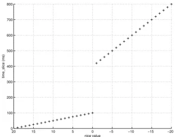
The Linux2.6kernel task scheduler has two priority queues, one for active tasks, and one for expired tasks. The queues are arrays of linked lists, one list for every priority. The scheduler always chooses the list with the highest priority in the active queue. Every task in the active queue of the system gets to run a certain time before it is put in the expired queue. This time is called a time_slice and the actual size of it depends solely on thenicevalue given to the task and not on the effective priority.Nicevalues in the interval [−20. . .0. . .19]are mapped to time slice sizes in the interval
[800ms . . .100ms . . .5ms]. The size of the resulting time slices can be seen in Figure 1. Note that the resulting time slices do not scale linearly with thenicevalue.
A non–interactive task is moved to the expired queue when it has used up its given time slice, an interactive task on the other hand is reinserted into the active queue if there is no risk of starvation in the expired queue. When there are no more tasks left in the active queue, it is switched with the expired one. The expired queue is considered to be starving if the first expired task has had to wait for more than a fixed
−20 −15 −10 −5 0 5 10 15 20 0 100 200 300 400 500 600 700 800 nice value time_slice (ms)
Fig. 1. The size oftime_sliceas a function of thenicevalue. Notice that thenicevalues are ordered from negative to positive values to indicate increasingtime_sliceallocation.
time multiplied with the number of tasks in the active queue. This makes the starvation–limit load dependent. It is also considered to be starvation if a task with lower nice value than the currently running task is in the expired queue.
Tasks with the same priority are treated differently, depend-ing on whether the scheduler considers them to be interactive or not. Non–interactive tasks are not interrupted by tasks with the same priority during execution of their time slice. Interactive tasks on the other hand get their time slice split up into smaller pieces, and are put at the end of the active queue again and again until they have executed for their whole time slice. The result is that interactive tasks are scheduled more or less round–robin with tasks of the same priority, while non– interactive tasks run non–preemptively.
For a more detailed description of the task scheduler, see [1]. IV. MODEL OF THESYSTEM
To start with, we assume that a task always needs to run, i.e., it is cpu–bound. We can then summarize the above in a few points and build a model of the system to predict its behavior.
• A task’s time slice depends solely on its nicevalue. • Tasks are scheduled in order of priority.
• Tasks are moved from the active queue to the expired queue when they have executed their whole time slice. • The active queue is swapped with the expired when
empty.
According to the model, the fraction of execution time that a task gets during one round of execution is calculated as:
f raction(i) =Ptime slice(i)
∀jtime slice(j)
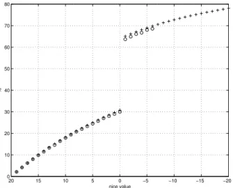
−20 −15 −10 −5 0 5 10 15 20 0 10 20 30 40 50 60 70 80 nice value %
Fig. 2. Comparison of the execution time model for Linux (+) and measurements on a computer (◦). Notice that thenicevalues are ordered from negative to positive values.
Example:If, for example, tasks1,2and3havenicevalue
0 and task4has nicevalue−1, then task4 will get:
f raction(i) = 420
100 + 100 + 100 + 420 ≈58%
A. Evaluation of the Model
To show that the model is accurate, theoretical values from the proposed model are compared to values received through measurements. The experimental setup consists of four tasks running in endless while–loops. Three of the tasks havenice
value 5, while thenicevalue of the fourth task is varied in
order to give it more or less CPU bandwidth compared to the other tasks. The result can be seen in Figure 2. Using lowernicevalues than−6 resulted in the system becoming
to sluggish to do any good measurements, therefore these are left out. This sluggishness is probably due to the fact that tasks with that low nicevalues are given so high priorities that they conflict with the tasks interacting with the user. As can be seen, the results from the experiments follow the model very well.
V. CONTROLLERIMPLEMENTATION
The control signal, in this case thenice value, can only change in discrete steps. This makes it impossible to keep some references statically. But by using modulation tech-niques, as for example Pulse Width Modulation (PWM), the reference can be kept on average. Another thing that one should be aware of is the nonlinearity in how thenicevalue is mapped to the time_slice, as seen in Figure 1. This makes it harder to follow references which forces the control signal to oscillate over the interval[0,−1]. Ongoing work is
to compensate this by an inverse–nonlinearity, and thereby reducing the oscillations. This will require more code to be executed in the kernel, but the overhead is expected to be fairly small.
A PI–controller with anti–windup has been implemented using fixed point arithmetic in a kernel module. The PI– controllers have a strong history in the control community because it combines robustness and fast response, while being relative simple to configure, even without exact knowledge of the system to be controlled. In the future, more elaborate schemes could be used that take into account more details of how the scheduler works, as well as global knowledge of the behavior of other tasks. By using a PI–controller in this way, a PWM–like behavior is achieved automatically. The implemented PI–controller is given by
u(k) = K yref −y(k)+I(k) (1)
I(k) = I(k−1) +TS
K Ti
yref−y(k) (2)
where the parameters K and Ti are the proportional and
integral control parameters, respectively. The variableuis the control signal (the nice value), and y is the measurement (the fraction of time given to the task). The variable k is the discrete time index, such that t =kTS, where TS is the
sampling time. The PI controller consists of two components. The proportional part (K(yref −y(k))) ensures fast reaction
to disturbances, but does not assure that the desired reference is reached. The integral part (described byI) will accumulate any error between the measurement and reference in a similar manner as an incremental controller. This part is particular beneficial when the system under consideration is not well– known and predictable, as with computer systems. The specific implementation uses the control parameters K = 0.01 and Ti= 52, and sampling times ofTS = 20ms.
Since the control design is not based on a dynamical model, there are no theoretical guarantees for performance or stability. However, the values of K and Ti have been chosen rather
conservatively to have large stability margins. This is imposed because even small changes to the nice value can lead to
large changes in the achieved CPU–bandwidth. The effect of changes to thenicevalue also varies with the number of tasks in the system and their respective nice values in turn. The fact that there are unknown parameters in the system makes it good to have a conservatively tuned controller. Another thing that makes a conservatively tuned controller preferable, is the fact that measurements are not taken instantaneously, but over an interval. The system must therefore be given some time to react to the control signal before changing it again. Using a large value onTi, also has the bonus effect that measurements
are averaged. In the case where the controller saturates, the control objective might not be met, since the controller lacks actuation possibility. The integral part will remain within the allowed control range due to the anti–windup scheme.
For more details on the controller implementation, see [1]. VI. TAKING THETASK’SSTATEINTOACCOUNT Up until now it has been assumed (for simplicity) that a controlled task is always willing to run, i.e., it is cpu– bound. This may be true in some cases, but obviously not in all. Imagine for example that the controlled task is given
a reference of 50%, but does not need more than 40% due to the fact that it is waiting on some I/O to occur the rest of the time. The integral part of the PI controller will then add up the difference, and increase the control signal in order to remove the error. But as the task is unwilling to run, and the system can not force it, the error will remain and the control signal will, due to the integral effect, continue to rise until it hits its limit. This is of course not a satisfactory behavior, and could be avoided by taking the current state of the task into account when controlling it. The strategy could be something like: do not increase the control signal further if the task is not not willing to run more. This is more or less an anti–windup scheme which ensures that the integral part does not wind up trying to enforce higher CPU allocation to a task than the task demands. The remaining part of this section will give a strategy for solving these kinds of situations.
A. Strategy
The idea to update the control signal only if the task is willing to run, sounds good at first. It is, however, not as simple as it first might seem. The obvious question to answer is: how do we know if a task is willing to run more than it already does? The idea used in the current controller implementation is to sample the state of the task at the same time as the execution time. The controller is then only executed if two consecutive samples show that the task is in the “running” state. This strategy works well if the task is usually in the “running” state for a longer time than the time between two consecutive samples of the controller. How long time a task spends in its “running” state depends highly on its workload during that time interval, but it also depends on the other tasks in the system, as the task might get interrupted by a higher priority task. This makes it hard to give any general rules and hence draw any conclusions to be used for more accurate control.
B. Why does the Strategy Work?
The reason why the strategy works, i.e., the control signal does not saturate, is the following: A task with a low priority will be in the “running” state for a long time. This is due to the fact that it will be preceded and interrupted by tasks with higher priorities. It will not switch from the “running” state until it has finished its current work load. If the priority of the task is increased, the task may not be preceded by as many tasks as before and it will also not be interrupted by as many. Hence, it will finish earlier and therefore be a shorter time in the “running” state. In essence, a high priority gives a short time in the “running” state. As the execution time demand is constant, the ratio between executed time and time spent in the “running” state will increase if the priority is increased. At a certain point, an equilibrium will be reached, where the reference is met during the period when the task is in the “running” state, and hence the control signal will be constant.
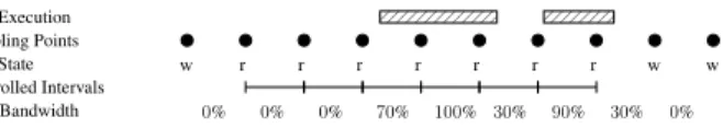
Example:Fig. 3 shows the sampling points of the controller,
and the task’s state at those points. It also shows the task’s execution trace and which of the sample intervals that are used
0000000 1111111 00001111 Task Execution Sampling Points Task State Controlled Intervals CPU Bandwidth r r r r r r r w w w 0% 0% 0% 70% 100% 30% 90% 30% 0%
Fig. 3. Figure showing how the strategy described in Section VI-B for controlling non–cpu bound tasks works.
by the controller. Anrmeans that the task is in the “running” state, and a wthat it is in one of the “waiting” states. During the controlled intervals, the ratio between executed time and time spent in the “running” state is approximately48%.
VII. EXPERIMENTS WITHLOADTASKS
Experiment 1 and 2 have been performed on a single CPU desktop computer. At the same time as the experiments were made, there were a number of tasks in the system, e.g., X, Firefox, Thunderbird, XEmacs and so on. All bandwidth measurements have been filtered through a moving average window of 4 s. The filtering is done because of the fact that when a task executes, it gets100% of the CPU–bandwidth and then it gets0% when it does not execute. Filtering through a moving average window shows the CPU–bandwidth during that window and this is also what one wants to achieve.
Running the experiments on a computer with more than one CPU will gain results similar to the ones seen in this section, except that there will considerably more load disturbances, as those seen in Experiment 1.
Experiment 1: The setup in this experiment consists of four
tasks running in endless while–loops. Two of the tasks have theirnicevalues set to five, and act as background load. The third and fourth task’snices values are used as control signals to keep the measured bandwidth at the desired references.
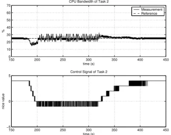
The references for both of the tasks are kept at25% initially. At time 182, the reference for the first task is changed from 25% to 50%. At around time 320, the reference is changed back to25%. The result of the step response for the first task can be seen in Figure 4. The coupling between the two tasks is visible in Figure 5, which shows the disturbance on the second task resulting from the step on the first one. No feed– forward term is used in the controller. This experiment shows the PWM nature of the control signal and the results of the quantization in the nice value. In Figure 4, it can be seen that the control signal is constant both before and after the two steps. But when the reference is set to50%, the control signal fluctuates a lot. Also note that there is much less oscillation in the CPU–bandwidth when the reference is set to 25% than to50%. This is due to the fact that some references cannot be kept stationary because thenicevalue is discrete.
Experiment 2: This experiment consists of one periodic
task that executes for approximately40ms and then sleeps for 60ms repeatedly. This results in a task that uses at most40% of the CPU even if it is alone in the system. Controlling such a task requires the state of the task to be taken into account as described in Section VI. Two load tasks of the same type used in Experiment 2 are also present in the system.
150 200 250 300 350 400 450 0 10 20 30 40 50 60 70
CPU Bandwidth of Task 1
% time (s) 150 200 250 300 350 400 450 −5 0 5
Control Signal of Task 1
nice value
time (s)
Measurement Reference
Fig. 4. Step response of the CPU bandwidth (task 1) when controlling two tasks in Experiment 1. 150 200 250 300 350 400 450 0 10 20 30 40 50 60 70
CPU Bandwidth of Task 2
% time (s) 150 200 250 300 350 400 450 −5 0 5
Control Signal of Task 2
nice value
time (s)
Measurement Reference
Fig. 5. Step response of the CPU bandwidth (task 2) when controlling two tasks in Experiment 1.
As can be seen in Figure 6, the proposed scheme works well in practise. In the beginning of the plot, the reference is higher than the task demands, and at time 55 it is set to an even higher value, but the control signal still behaves well. It can also be seen that the controller is still able to follow reference changes when they are lower than40%.
The observant reader may notice the delay and the following under–shoot at time160. Also note that this behavior does not show up at any of the other step changes in the plot. This is not an integrator windup as might first be thought, but is instead due to the fact that the system has marked the task as interactive and therefore given it an additional bonus. When the task after some time is marked as non–interactive, it loses its bonus and this results in the under–shoot.
0 50 100 150 200 250 300 350 400 450 0 20 40 60 80 CPU Bandwidth % time (s) 0 50 100 150 200 250 300 350 400 450 0 5 10 15 20 Control Signal nice value time (s) Measurement Reference
Fig. 6. Step responses for a non cpu–bound task when taking the task’s state into account in Experiment 2.
VIII. EXPERIMENT WITHAPACHESERVERS This experiment aimed to test the scheduling mechanism on a more realistic application. The test is not included to suggest that the mechanism is the best solution for the given example, but only to demonstrate that the method works for a problem including more advanced behavior than the previous tests.
The setup represents a hosting system where two service providers are hosted on the same physical hardware. The objective is to separate the two service providers such that one service provider can operate unaffected of a request overload at the other service provider.
Experiment 3: A Pentium 4, 1 GB memory, 3 GHz PC,
with a Linux Fedora 5 operating system and kernel 2.6.17. was used as host computer. Two Apache servers, version 2.2.2, configured by using the prefork module, were installed on the server as two distinct service providers. Using this configuration, a request was handled by one process (child). If all existing processes were occupied, Apache dynamically started new processes, and likewise, closed some if there were too many idle processes. This means that the number of processes associated with one Apache server changed over time. The controller was configured to set a common nice
value to all the processes of a given Apache server. Also, the time allocated to all the processes of one Apache serve were summed to give the time fraction measurement. In this manner, a single–input single–output system was obtained as required by the control structure. Only one of the Apache servers was controlled with the proposed scheduling mechanism. The controlled and uncontrolled server were listening on port 80 and 81, respectively. The setup is illustrated in Figure 7.
Traffic was generated from 12 client computers (Athlon, 1.5 GHz PC), grouped into three equal groups consisting of four client–computers each. The traffic was generated using the traffic generation software CRIS [2]. All clients requested the same PHP file (generating a response with 7000 characters)
Port 80 Server Uncontrolled Client #12 Client #1 · · · Port 81 Controlled Server Arrival intensity Time Arrival intensity Time
100 Mbit switched network TCP/IP layer Host computer
Fig. 7. Experimental setup for experiment 3.
with exponentially distributed inter–arrival times, and were configured to timeout after 10 s. During the experiment, all the computers were connected on a 100 Mbit switched Ethernet network.
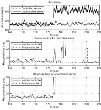
At the beginning of the experiments, client group I started sending requests to the controlled server and client group II started to sent requests to the uncontrolled server. Both groups sent approximately 160 requests/s. This traffic did not give rise to CPU–overload, but left approximately 25% CPU bandwidth free. A server is considered to be overloaded when the requests can not be served within the timeout of the clients due to lack of CPU resources. After 173 s, client group III started to send approximately 160 requests/s to the uncontrolled server. The computer did not have sufficient CPU capacity to maintain operation of both servers. The averaged arrival–intensity is shown in the uppermost sub–figure of Figure 8. The traffic going to the uncontrolled server was the combined traffic from client group II and III.
Under the initial operation none of the servers were over-loaded but as the request rate to the uncontrolled server was doubled, the computer lacked the CPU bandwidth to serve all requests. Preferably, only the server being exposed to the extra traffic should become overloaded, while the other server should remain operational.
The middle and bottom sub–figures of Figure 8 show the response times of the controlled server and the uncontrolled server, respectively. In the case where the controller was inactive, both servers became overloaded when the traffic increased. After the increase of traffic, the response times of both servers increased dramatically and all clients started to timeout. Consistent timeouts from the clients were observed. In the case where the CPU resource allocation was controlled by the proposed scheduling mechanism (reference set to 45% CPU bandwidth), only the uncontrolled server became over-loaded. The controlled server continued to perform with simi-lar response times. Client timeouts were observed consistently only on the uncontrolled server’s requests. Two single timeouts were observed on the controlled server’s requests. The small
140 150 160 170 180 190 200 210 100
200 300
Time (s)
Arrival rate (req/s)
Arrival rate Controlled server Uncontrolled server 140 150 160 170 180 190 200 210 0 20 40 60 Time (s) Response time (ms)
Response time for controlled server
Inactive controller Active controller 140 150 160 170 180 190 200 210 0 20 40 60 Time (s) Response time (ms)
Response time for uncontrolled server
Inactive controller Active controller
Fig. 8. Results from experiment 3 on two Apache servers. Top: Average arrival rates. Middle: Response time for the controlled server with and without feedback control. Bottom: Response time for the uncontrolled server. All variables were measured at the clients and were filtered with a moving average window of 200 requests.
jump observed in the response time of the controlled server (middle sup–figure of Figure 8) at around 200 s is assumed to be due to some disturbance from other tasks in the operating system.
This experiment showed that the scheduling mechanism can be used to affect the response time of a web server application. The setup with two different servers with different client groups can be used in applications where different sites are hosted on the same physical computer, but where the performance of one server must be independent of the behavior of the other server. In this experiment we have not considered how such a system should be setup in a real application. For instance, we do not consider how the traffic to the two servers is separated. However, the experiment shows that the two servers can be separated by means of the proposed scheduling mechanism. The setup does not aim to control the response time. If this was the objective, a second control loop would have to be included, defining the reference for the CPU– bandwidth controller.
IX. RELATEDWORK
Reservation based scheduling is not a new concept and has been around in one form or another for many years. The concept has been called fair–share scheduling [3], [4], [5] but is also known under the name proportional–share
scheduling [6], [7], [8], [9]. A good summary of this field,
together with more details can be found in [10].
The idea of using thenicevalue as a way to enforce CPU fractions has been known before. One early implementation is the Watson Share scheduler [11], implemented on top
of a standard AIX operating system at the Compute Power Server Cluster at IBM. It is also mentioned in [12] and [13] as something that in UNIX can be done in theory, but is complicated in practice because of the non–linear relationship betweennice, the number of processes and the CPU fraction
received. Provided that the number of jobs in the system is fixed, and that they are all present from the same time and onward, a deterministic analysis of the steady state shares is possible. [14] shows how this can be used to statically calculate the base priorities on a uniprocessor in the presence
ofdecay–usage schedulinginUNIX. [15] extends this analysis
to the multiprocessor case.
An interesting Linux kernel project in this area is Class–
based Kernel Resource Management (CKRM) [16] and [17]
which aims at providing differentiated service to resources such as CPU bandwidth, memory pages, I/O and incoming network bandwidth. It accomplishes CPU reservations by scaling the time_slicevalue and re–queuing tasks. Parts of this project is used in “SuSE Linux Enterprise Server 9”, but not the CPU controller.
Resource allocation and reservation in web server applica-tions is nothing new. An example is [18] where virtual serving on one physical computer is used to guarantee certain quality of service metrics for several client classes under chancing load conditions. An often used actuation method is admission control, where requests are denied in order to avoid overload and to guarantee certain performance metrics for the accepted requests [19], [20], [21].
X. CONCLUSIONS
An exposition of the Linux2.6scheduler has been done and a feedback–based method for controlling the CPU bandwidth given to tasks in Linux has been presented. The presented method has been shown to work, both for cpu–bound and non cpu–bound tasks. A number of experiments have been performed in order to show that the technique works in real-ity. The experiments indicate that CPU bandwidth allocation can be obtained with the proposed scheduling mechanism. Furthermore, the mechanism can be used to separate the performance of two Apache servers running on the same physical computer—that is, one server remains operational while the other server is overloaded.
REFERENCES
[1] M. Ohlin, “Feedback Linux scheduling and a simulation tool for wireless control,” Department of Automatic Control, Lund University, Sweden, Licentiate Thesis ISRN LUTFD2/TFRT- -3240- -SE, June 2006. [2] M. Andersson, A. Hagsten, and F. Neisler, “Crisis request generator for
internet servers,” inProc. Fourth Swedish National Computer Network-ing Workshop, Lule, Sweden, 2006.
[3] R. B. Essick, “An Event-Based Fair Share Scheduler,” inProc. of the Winter 1990 USENIX Conf. USENIX, 1990, pp. 147–162.
[4] J. Kay and P. Lauder, “A fair share scheduler,”Communications of the ACM, vol. 31, no. 1, pp. 44–55, 1988.
[5] G. J. Henry, “The Fair Share Scheduler,” AT&T Bell Laboratories Technical Journal, vol. 63, no. 8, pp. 1845–1857, October 1984. [6] L. L. Fong and M. S. Squillante, “Time-Function Scheduling: A
Gen-eral Approach to Controllable Resource Management,” IBM Research Division, T.J. Watson Research Center, Yorktown Heights, NY 10598, Tech. Rep. RC 20155 (89194), August 1995.
[7] I. Stoica and H. Abdel-Wahab, “Earliest Eligible Virtual Deadline First : A Flexible and Accurate Mechanism for Proportional Share Resource Allocation,” Norfolk, VA, USA, Tech. Rep., 1995.
[8] C. A. Waldspurger and W. E. Weihl, “Stride Scheduling: Determinis-tic Proportional-Share Resource Mangement,” Massachusetts Institute of Technology, MIT Laboratory for Computer Science, Tech. Rep. MIT/LCS/TM-528, June 1995.
[9] ——, “Lottery Scheduling: Flexible Proportional-Share Resource Man-agement,” inFirst Symp. on Operating Systems Design and Implemen-tation (OSDI). USENIX Association, 1995, pp. 1–11.
[10] J. de Jongh, “Share Scheduling in Distributed Systems,” Ph.D. dissertation, Delft University of Technology, 2002. [Online]. Available: http://www.pds.ewi.tudelft.nl/pubs/ph d/dejongh.pdf
[11] C. Moruzzi and G. Rose, “Watson Share Scheduler,” inProc. of the Fifth Large Installation Systems Administration Conf. (LISA ’91). San Diego, USA: USENIX, 1991, pp. 129–133.
[12] J. L. Hellerstein, “Challenges in Control Engineering of Computing Systems,” inProc. of the 2004 American Control Conf., vol. 3, 2004, pp. 1970– 1979.
[13] J. L. Hellerstein, Y. Diao, S. Parekh, and D. M. Tilbury, “Control Engineering for Computing Systems,”IEEE Control Systems Magazine, vol. 25, no. 6, pp. 56–68, dec 2005.
[14] J. L. Hellerstein, “Achieving Service Rate Objectives with Decay Usage Scheduling,”IEEE Trans. Software Eng., vol. 19, no. 8, pp. 813–825, 1993.
[15] D. H. J. Epema, “Decay-Usage Scheduling in Multiprocessors,” ACM Trans. Comput. Syst., vol. 16, no. 4, pp. 367–415, 1998.
[16] CKRM, “Class-based Kernel Resource Management (CKRM),” Home page: http://ckrm.sourceforge.net/, 2006.
[17] S. Nagar, R. V. Riel, H. Franke, C. Seetharaman, V. Kashyap, and H. Zheng, “Improving Linux resource control using CKRM,” inProc. of the 2004 Linux Symp., vol. 2, Ottawa, Ontario, Canada, July 2004, pp. 511–524.
[18] W. Xy, X. Zhu, S. Singhal, and Z. Wand, “Predictive control for dynamic resource allocation in enterprise data centers,” inProc. Conf. on Management of Integrated End-to-end Communications and Services, NOMS, Vancouver, Canada, April 2006, pp. 115–126.
[19] X. Chen, H. Chen, and P. Mohapatra, “Aces: An efficient admission control scheme for qos-aware web servers,”Computer Communications, vol. 23, no. 14, pp. 1581–1593, 2003.
[20] S. C. Lee, J. C. Lui, and D. K. Yau, “A proportional-delay diffserv-enabled web server: admission control and dynamic adaptation,”Parallel and Distributed Systems, IEEE Trans., vol. 15, no. 5, pp. 385–400, 2004. [21] M. Andersson, J. Cao, M. Kihl, and C. Nyberg, “Admission control with service level agreements for a web server,” inProc. of IASTED Int. Conf. on Internet and Multimedia Systems and Applications (EuroIMSA), Grindelwald, Switzerland, February 2005.