Accelerating Mobile Audio Sensing Algorithms through On-Chip GPU Offloading

Accelerating Mobile Audio Sensing Algorithms

through On-Chip GPU Offloading

Petko Georgiev

, Nicholas D. Lane

, Cecilia Mascolo

, David Chu

University of Cambridge,†

University College London,∗

Nokia Bell Labs,‡

Google

ABSTRACT

GPUs have recently enjoyed increased popularity as general pur-pose software accelerators in multiple application domains includ-ing computer vision and natural language processinclud-ing. However, there has been little exploration into the performance and energy trade-offs mobile GPUs can deliver for the increasingly popular workload of deep-inference audio sensing tasks, such as, spoken keyword spotting in energy-constrained smartphones and wearables. In this paper, we study these trade-offs and introduce an optimiza-tion engine that leverages a series of structural and memory access optimization techniques that allow audio algorithm performance to be automatically tuned as a function of GPU device specifications and model semantics. We find that parameter optimized audio rou-tines obtain inferences an order of magnitude faster than sequential CPU implementations, and up to6.5x times faster than cloud of-floading with good connectivity, while critically consuming3-4x less energy than the CPU. Under our optimized GPU, conventional wisdom about how to use the cloud and low power chips is broken. Unless the network has a throughput of at least20Mbps (and a RTT of25ms or less), with only about10to20seconds of buffering au-dio data for batched execution, the optimized GPU auau-dio sensing apps begin to consume less energy than cloud offloading. Under such conditions we find the optimized GPU can provide energy benefits comparable to low-power reference DSP implementations with some preliminary level of optimization; in addition to the GPU always winning with lower latency.

1.

INTRODUCTION

Graphics Processing Units (GPUs) are the method of choice for executing high computational loads and accelerating compute-inten-sive applications in domains such as computer vision [55, 24, 37] and deep learning [17, 18]. But GPUs like any complex processor architecture need to be used smartly to maximize their through-put and efficiency. There have been extensive studies for graphics and games [55, 37, 55, 48] including mobile [24], but the analysis has largely evaded other general-purpose GPU computations on a mobile device such as audio applications that rely on the power-hungry microphone sensor. Examples of audio sensing apps are Permission to make digital or hard copies of all or part of this work for personal or classroom use is granted without fee provided that copies are not made or distributed for profit or commercial advantage and that copies bear this notice and the full cita-tion on the first page. Copyrights for components of this work owned by others than ACM must be honored. Abstracting with credit is permitted. To copy otherwise, or re-publish, to post on servers or to redistribute to lists, requires prior specific permission and/or a fee. Request permissions from [email protected].

MobiSys ’17, June 19–23, 2017, Niagara Falls, NY, USA

c

2017 ACM. ISBN 978-1-4503-4928-4/17/06. . . $15.00 DOI:http://dx.doi.org/10.1145/3081333.3081358

personal digital assistants such as Apple’s Siri [2] or Google Now [5], as well as a plethora of behavior monitoring apps that recog-nize emotions from voice [50, 44], or perform conversation anal-ysis [43, 56, 46]. These applications are capable of deep infer-ences about user behavior, often require continuous sensor monitor-ing, and boast highly sophisticated inference algorithms that easily strain scarce mobile resources(battery, memory and computation) [?]. As a result, computational offloading to cloud [25] or low-power co-processors [28, 43] has often been the solution applied to keep these apps functional on the mobile device, but no study has been done on the feasibility of GPU offloading for this data-intensive workload.

In the mobile landscape where energy is the biggest limiting fac-tor, it is not immediately obvious whether accelerating these sens-ing applications via GPU offloadsens-ing will result in energy-justified performance boosts compared to the above mentioned alternatives (cloud and low-power co-processors). Questions that we inves-tigate in this paper are: What trade-offs do we get in terms of speed and energy if we express audio sensing algorithms in a GPU-compliant manner? How can we best take advantage of the general-purpose computing capabilities of mobile GPUs to offload audio processing? When should we prefer GPU computation to cloud? Can we obtain energy efficiency on a scale comparable to a low-power Digital Signal Processor (DSP)?

In this work, we show that the GPU performance of audio sens-ing algorithms is sensitive to two key control-flow parameters such as the frame fan-out (total number of frame processing GPU threads) and per-thread compute factors (amount of computation relative to memory accesses). We present a GPU offloading engine that leverages parallel optimization techniques that allow us to control these parameters and auto-tune the performance of audio routines. Without such optimization, naively parameterized GPU implemen-tations may be up to1.5x slower than multi-threaded CPU alterna-tives, and consume more than2x the energy of cloud offloading.

Through extensive evaluation we find thatfor time-sensitive au-dio apps, and when energy is less of a concern, there is no bet-ter option than using GPU optimized audio routines. Algorithms tuned for the GPU can deliver inferences an order of magnitude faster than a sequential CPU deployment, and3.1x or6.5x faster than cloud offloading with good connectivity for deep audio infer-ences such as speaker identification and keyword spotting, respec-tively. At the same time, the energy consumed is3-4x lower than when using the CPU. Perhaps more surprising,for tasks that are more continuous but tolerate short delays (of10-20secs) GPU is also a top choice. When raw data is accumulated for batched pro-cessing, algorithms optimized for the GPU begin to consume less energy than cloud offloading with fast connections. Further, the op-timized GPU can deliver energy efficiency levels in ranges

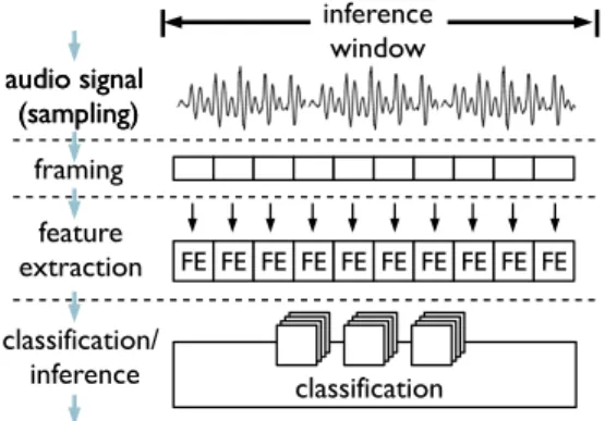
compa-inference window audio signal (sampling) audio signal (sampling) framing FE FE FE FE FE FE FE FE FE FE feature extraction classification classification/ inference

Figure 1:Audio pipeline structure.

rable to what can be achieved by low-power DSP implementations with some preliminary optimization. The batching delays required for the benefits to appear are sufficiently short to support the opera-tion of not only life-logging style behavior monitoring applicaopera-tions that tolerate large delays, but also apps that deliver context aware services and notifications such as conversation analysis [56, 41].

The contributions of our work are:

• A detailed study of the trade-offs of using mobile system-on-a-chip GPUs for audio sensing workloads.

• An optimization engine that uses key structural and memory ac-cess parallel patterns applicable to popular algorithm building blocks used in numerous audio sensing apps available commer-cially and in the literature. These patterns allow us to automat-ically tune the GPU performance boost of audio pipelines: they 1) increase the data parallelism by allowing a larger number of threads to work independently on smaller portions of the au-dio input stream; and 2) strategically place data needed by the threads into GPU memory caches where access latency is lower and the data can be reused.

• A comprehensive proof-of-concept OpenCL [12] implementa-tion of widely used audio sensing algorithms built on a smart-phone development board [16]. Our prototype includes a library of sensing components for feature extraction and classification (including DNNs [35], GMMs [19] etc.) needed for common forms of context inference. These components serve as the build-ing blocks for numerous apps from the audio processbuild-ing litera-ture – as a demonstration, we implement3 recently proposed application pipelines (e.g., emotion recognition, speaker identi-fication and spoken keyword spotting).

To the best of our knowledge, we are the first to identify gener-alizable GPU parallel optimizations that areapplicable across mul-tiple algorithmsused in the unique workloads required by audio sensing. Previous efforts [58, 30] have focused on different work-load scenarios (e.g., automated speech recognition) where process-ing requirements differ from those imposed by audio sensprocess-ing: con-tinuous background monitoring of coarse sound classes supported by offline-trained models that can operate entirely cloud-free.

2.

AUDIO SENSING MEETS THE GPU

In this section, we detail the operation of typical microphone-based sensor apps, elaborate on the GPU execution model and high-light some of the challenges it presents for audio sensing.

2.1

Audio Sensing Primer

Audio sensing apps are characterized by their ability to sample and process microphone data – they include specialized audio

pro-cessing code that is distinctly different from the app specific logic (e.g., activating services based on detected audio context). The dataflow of sensor processing within these apps share many sim-ilarities which we illustrate in Figure 1. The execution begins with the sampling of the microphone where raw data is typically accu-mulated over a short time window (hundreds of milliseconds up to a few seconds) sufficient to capture distinctive characteristics of sounds and utterances. The audio signal is then subdivided into much shorter (e.g.,30ms) segments calledframeswhich are sub-ject to preprocessing and feature extraction. The aim of the features is to summarize the collected data in a way that describes the differ-ences between targeted behavior or context (e.g., sounds, words, or speaker identity). Identifying which activity or context is observed in the sensor data in the analyzed time window requires the use of one or more classification models. Models are usually built offline prior to deploying a sensor app based on examples of different ac-tivities and often the classification (i.e., model evaluation applied to the whole window of stacked frame feature data) is a bottleneck stage of the audio pipeline [28]. Example audio apps with their execution properties are listed in Table 1.

2.2

Example Audio Applications

Two most widely used classification models in the audio sensing domain are Gaussian Mixture Models (GMMs) and Deep Neural Networks (DNNs). Table 2 gives instances of their near ubiquitous usage. Here we describe the operational semantics of3 representa-tive data-intensive deep-inference examples built on these models. However, we note that the techniques we develop are applicable to any other audio sensing application from Table 2 that uses these models as a building block.

Speaker Identification (GMM based). The pipeline is introduced by Rachuri et al. [50]. Gaussian Mixture Model classifiers are trained using speech from23speakers. Each of the speakers is represented by a speaker-specific GMM built by performing Max-imum a Posteriori (MAP) adaptation of a 128-component back-ground GMM representative of all speakers. The GMM evaluates the probability with which certain acoustic observations match the model and in our case these observations are32Perceptual Lin-ear Prediction (PLP) coefficients [33] extracted from30-ms frames over 5seconds of recorded audio. At runtime, the likelihood of the audio sequence is calculated given each speaker model and the speaker with the highest likelihood is predicted.

Emotion Recognition (GMM based). Structurally, the pipeline is identical to the Speaker Identification. The difference comes from the parameters of the GMMs which are trained on a differ-ent dataset (the Emotional Prosody Speech and Transcripts library [42]) so that each GMM represents an emotional category [50]. Keyword Spotting (DNN based). The application is based on the small-footprint implementation of Chen et al. [23], and its aim is to detect a hot phrase spoken by a nearby speaker. The example ap-plication is trained to detect an "Ok, Google" command. The audio analysis is performed by segmenting the input signal into frames of length25ms with an offset of10ms, i.e. the frames overlap. Filter-bank energies (40coefficients) are extracted from each frame and accumulated into a group of40frames. The features from these frames serve as the input layer to a DNN with as many output layer nodes as there are target keywords (plus an additional sink node to capture other words). The DNN is fully connected and has3hidden layers with128nodes each. The output of the DNN is raw poste-rior probabilities of encountering each of the keywords over the last second of data. The DNN feed forwarding is performed in a

slid-Application Purpose Main Features Inference Model Frame Window

Emotion Recognition∗[50] emotion recognition PLP∗[33] 14Gaussian Mixture Models∗[19] 30ms 5s Speaker Identification∗[50] speaker identification PLP∗ 23Gaussian Mixture Models∗ 30ms 5s Keyword Spotting∗[23] hotphrase recognition Filterbank Energies∗ Deep Neural Network∗[35] 25ms 1s Stress Detection [44] stress from voice MFCC [27], TEO-CB-AutoEnv [59] 2Gaussian Mixture Models∗ 32ms 1.28s

Speaker Count [56] speaker counting MFCC, pitch [26] Unsupervised Clustering 32ms 3s Ambient Sound Classification [45] sound recognition MFCC, Time Domain Features Gaussian Mixture Models∗ 64ms 1.28s

Table 1:Example audio sensing applications and their properties.∗Apps and models implemented in OpenCL.

Classifier Applications

GMM emotion recognition [50], speaker identification [50, 43], ambient sound classification [45], stress detection [44] DNN keyword spotting [23], emotion recognition [31], speech

recognition [34], sound event classification [47]

Table 2: Categorization of audio sensing applications based on classification model.

Work Item

Work Group ND Range

SP

Waves

Figure 2:OpenCL thread model and a GPU Shader Processor. The SP features2waves of8work items each, it can run16threads in total simultaneously. The work items of one work group are executed on a single SP.

ing window with every new frame, resulting in100propagations per second (once every10ms).

2.3

GPU Execution Model and Challenges

We use OpenCL’s terminology [12] and Qualcomm Adreno GPU [13] as an example for GPU architecture and programming model, but our discussion and conclusions apply equally to other GPU plat-forms, such as NVIDIA with CUDA [9]. To an OpenCL program-mer, a computing system consists of ahost that is traditionally a CPU, such as the Snapdragon 800 Krait CPU, and one or more devices(GPU) that communicate with the host to perform paral-lel computation. Programs written in OpenCL consist of host code (C API extensions) and device code (OpenCL C kernel language) – communication between the two is performed by issuing com-mands to a command queue through the host program space. Ex-ample commands are copying data from host to device memory, or launching akernelfor execution on the device. Kernels specify the data-parallel part of the program that will be executed by the GPU threads. When a kernel is launched, all the threads execute the same code but on different parts of the data.

Thread Model and Compute Granularity. All the threads gen-erated when the kernel function is called are collectively known as a grid (or ND Range) and are organized in a two-level hierarchy independently from the underlying device architecture. Figure 2 il-lustrates this organization. The grid consists ofwork groupseach containing a set of threads known aswork items. The exact thread scheduling on the GPU is decoupled from the work groups and is vendor specific although it shares a lot of similarities among GPU varieties. Switching from a group of work items to another occurs when there is a data dependency (read/write) that must be com-pleted before proceeding and is done to mask these IO latencies.

One of the challenges of implementing GPU-friendly algorithms is providing the right level of work item granularity. If the GPU

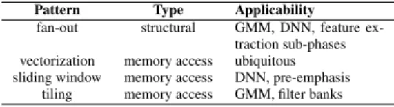
Pattern Type Applicability

fan-out structural GMM, DNN, feature ex-traction sub-phases vectorization memory access ubiquitous sliding window memory access DNN, pre-emphasis

tiling memory access GMM, filter banks

Table 3:Parallel optimization patterns taxonomy.

threads are too few, the GPU will struggle with hiding memory access latency due to not being able to switch between compute-ready threads while others are stalled on a memory transaction. Audio sensing algorithm execution revolves around the analysis of frames, and a natural candidate for data parallelization is to let each work item/thread analyze a frame. However, the number of frames in an inference window is on the order of tens to hundreds, whereas the GPU typically requires thousands of threads for any meaningful speedups to begin to appear. A challenge is organizing the audio al-gorithm execution in a way that allows more work items to perform computation.

Managing Memory-Bound Audio Kernels. Work items have ac-cess to different memory types (global, constant, local/shared, or private) each of which provides various size vs. access latency trade-offs. Global memory is the largest but also the slowest among the memories. Private memory is exclusive to each work item and is very limited in size, whereas the shared memory is larger and accessible by all work items in a group. Often, acompute to global memory access (CGMA) ratiois used as an indicator of the kernel efficiency – the higher the ratio is, the more work the kernel can perform per global memory access, the higher the performance.

Typical algorithms used in audio sensing need to read a large number of model parameters which they apply to the frame data, but the number of floating point operations per read is relatively low making audio kernelsmemory-bound. In order to squeeze max-imum performance out of the mobile GPU (highest speed and thus lowest energy consumed), algorithms will need to reduce the global memory traffic by intelligently leveraging the smaller but lower access latency memories (shared and private). The challenge is enabling appropriate memory optimization strategies that keep the CGMA ratio high while maintaining a suitable level of granularity for the work items.

Summary. GPUs are a powerful platform for general-purpose computing programmed by language abstractions such as OpenCL and CUDA. An unanswered challenge is how and what perfor-mance control techniques we can leverage that depend on the al-gorithm semantics rather than a concrete hardware configuration.

3.

OPTIMIZATION ENGINE OVERVIEW

To address the GPU deployment challenges presented in the pre-vious section, we build a library of OpenCL auto-tunable audio rou-tines that form the narrow waist of audio processing pipelines found in the mobile sensing literature (e.g., filter bank feature extraction, Gaussian Mixture Model, Deep Neural Network inference). This

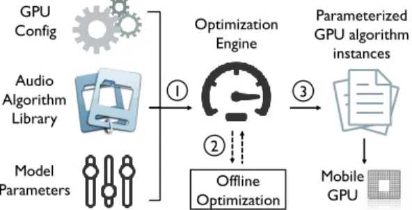
GPU Config Audio Algorithm Library Model Parameters Optimization Engine Parameterized GPU algorithm instances Offline Optimization Mobile GPU 1 2 3

Figure 3:High-level optimization engine workflow. library builds upon a set of structural and memory access tech-niques that expose a set of tunable audio model-dependent control-flow parameterswhich we can control in a pre-deployment step with an optimization engine. The goal of this engine is to provide the best match between the domain-specific library implementa-tion and mobile GPU hardware constraints. The engine helps to avoid cumbersome hand tuning, instead automatically finds optimal parameters for the audio kernel routines with large performance boosts for some of the algorithms. This requireszerochange in the kernel code itself, the parameters are passed through OpenCL commands as kernel arguments at runtime. A high-level workflow is illustrated in Figure 3.

The pre-deployment step is a three-staged process, where the en-gine first loads as input audio model parameters such as the DNN layout and queries the GPU device specification (e.g., GPU shared cache size) in order to be able to estimate optimum values for the GPU algorithm control-flow parameters. In the second stage, the engine performs the optimization step by solving a series of linear and quadratic equations and outputs a configuration file with GPU-kernel parameter values required by our audio library. The third stage is loading the values from the locally persisted config file to parameterize the audio algorithms upon initialization of concrete sensor apps.

To provide high-performance parallel implementations, we build the techniques listed in Table 3 that enable control over the follow-ing parameters. Empirically we found that for memory-bound au-dio kernels, these provide a sweet spot of tunable but not too com-plex parameters with a key impact on mobile GPU performance:

• frame fan-out factor (φ)– defined as the total number of au-dio frame processing GPU threads. A higher value results in an increase in the number of concurrent threads that can work inde-pendently.

• per-thread compute factor (κ)– defined as the number of com-puted output values per GPU thread. By optimizing this the engine attempts to maximize the number of computations each thread can perform relative to its memory reads and writes (fa-voring compute-bound operation instead of memory-bound). Manipulating the first parameter is achieved in our library through the frame fan-outstructural optimization pattern. The core idea behind it is to split the audio analysis so that each GPU thread can work on a subset of the output values extracted from an audio frame. The second parameter is tightly related to a set of memory access patterns that reduce expensive global memory traffic and in-crease the per-thread compute factor. These techniques are: 1) Vec-torizationthat consolidates slow global memory reads into a single load operation which is possible thanks to the sequential nature of accessing values from the audio stream. In our examples, the en-gine selects larger read batches and can fetch into the thread regis-ters up toxvalues from memory, wherexis vendor specific (for

Qualcomm Adrenox= 16, for NVidia Tegra X1x= 4[11]). 2) Memory Sliding WindowandMemory Tiling: the techniques allow threads to collaboratively load data into shared memory where this data can be subsequently reused with lower latency to produce mul-tiple output values. These are critical optimizations since global memory access is arguably the most prominent bottleneck we ob-serve in the widely used audio classification and feature extraction algorithms.

4.

PARALLEL CONTROL-FLOW

OPTIMIZATION

In this section, we detail the structural and memory access paral-lel patterns that enable the optimization engine to parameterize the audio routines in our library.

4.1

Inter- and Intra- Frame Fan-Out

This pattern controls the level of data parallelism by allowing a larger number of concurrent threads to perform independent com-putations on the input data. We can support such a mode of op-eration thanks to the way audio pipelines process frames – repeat-edly mixing the frame samples/coefficient with multiple parameters (GMM mixtures, DNN network weights). Independent computa-tions are performed not only among different frames but also within a single frame as well, a phenomenon which we call theframe fan-out. This allows the total amount of threads, orfan-out factor(φ), to be relatively high. It can be computed as follows: φ = n∗ν κ

wherenis the number of frames,νis the total number of output values per frame, andκis the number of computed values per GPU thread (per-thread compute factor). This structural optimization is applicable across both feature extraction (filter bank computation) and classification phases. The next two examples illustrate how this pattern can be applied:

GMM Fan-Out. The input for this classification phase is the ex-tracted feature coefficients from all frames. In the Speaker Iden-tification pipeline there are32PLP frame features and a total of n= 500frames per inference window (one frame every10ms for

5s). Each GMM hasν= 128mixtures each of which computes a probability score by mixing the32PLP coefficients from a frame with the parameters (mean and variance) of32Gaussian distribu-tions. With a per-thread compute factor ofκ= 1, we could let each OpenCL work item estimate the probability score for one mixture per frame resulting in a fan-out factor ofφ= 500×128. We enable the kernel to generate this massive number of work items by letting them write intermediate scores to global memory and a separate kernel is launched to sum the scores.

DNN Fan-Out. Similarly, the input data for the keyword spot-ting DNN classification is the extracted filter bank energies from the frames. In a1-second inference window there are a total of n = 100network propagations (one per new frame every10ms). A DNN kernel computes partial results across all input frames by performing the feed forward propagation for one layer across the frames simultaneously. Multiple kernels are launched each of which computes the node activation values for the next layer. Withν = 128nodes in the hidden layers we could let each OpenCL work item compute the activation for one node per frame offset (κ= 1) resulting in a fan-out factor ofφ= 100×128.

The role of the optimization engine is to provide optimum values for the control-flow parametersφandκ.nandνare determined di-rectly by the audio model specification, whereas the final value ofφ depends onκ, or the amount of work each GPU thread is assigned. The engine tunes the per-thread compute factorκsince we observe

Algorithm 1Shared Memory Use Kernel Template

1: Input: (i) Pointer to input buffer (in), (ii) Pointer to output buffer (out), (iii) Thread local id (lid), (iv) Thread group id (gid), (v) Shared memory maximum size (max_s).

.Collaborative data load: 2: loadOffset←compute_load_offset(lid)

3: inputOffset←compute_input_offset(gid,lid)

4: __shared floatNdata[max_s] .shared memory declaration 5: ifloadOffset< max_sthen

6: data[loadOffset]←vloadN(0, &in[inputOffset]) . vectorized

7: barrier(CLK_LOCAL_MEM_FENCE) .wait for all threads to finish loading data

.Shared data processing: 8: for (i= 0;i < x; + +i) do

9: localDataOffset←compute_local_offset(lid,i) 10: result←process(&data[localDataOffset]) 11: outputOffset←compute_output_offset(gid,lid,i) 12: out[outputOffset]←result

thatmaximum GPU performance may not necessarily be reached when parallelism is highest. The fan-out factorφreaches its max-imum when its denominator (κ) has its lowest value (κ= 1), i.e. when there are more threads performing less work. The memory access patterns in the following subsection enable each GPU thread to perform more computation (κ >1) relative to the number of its memory reads and writes: the total count of threads decreases but they can make a more efficient use of memory.

4.2

Memory Access Control

Tuning audio kernel performance with the per-thread compute factorκis closely related to how memory access is managed by the threads in a work group. Increasing the number of computa-tions per thread per global memory access and thus finding opti-mum values forκdepends on maximum exploitation of the faster but limited in size GPU memories. We discuss several key strate-gies, enabled by the specifics of digital signal processing, to lower the number of global memory operations. These strategies either 1) batch global memory transactions into fewer operations, or 2) let thethreads in a work group collaboratively load data needed by all of them into shared memory where access latency is lower. Vectorization. When kernels read the input data features or param-eters, for instance, they access all the adjacent values in a frame. As a result, the memory access can be vectorized and consolidated with vector load operations that fetch multiple neighboring val-ues at once from global to private memory. For example, when a thread requires the32PLP coefficients from a frame, it can use the OpenCLvloadxoperation to issue2reads with16values (vload16) fetched simultaneously instead of performing32reads for each co-efficient separately.

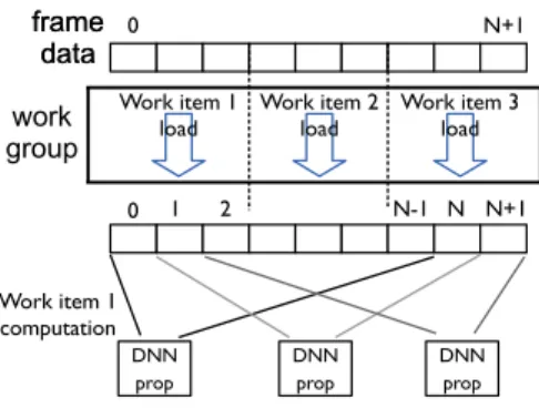
Shared Memory Sliding Window. Often the input raw audio or feature stream is processed in sliding window steps, i.e. the input is divided into overlapping frames over which identical computations are performed. Example scenarios where this type of processing is commonly applied are the feature extraction (PLP, MFCC [27]), or the classification of the feature stream into observed phenom-ena (as is the case for the DNN keyword spotting, see Figure 4). The data overlap is usually quite substantial – the feature extrac-tion phase for the Speaker Identificaextrac-tion pipeline, for instance, uses

30ms frames (240samples at a sampling rate of8kHz) with a10ms frame rate (an offset of80samples) resulting in a66%data over-lap between subsequent frames. We can exploit this property of the audio stream processing to let the threads in a work group

col-frame data

0 1 2 N-1 N N+1

Work item 1

load Work item 2load Work item 3load work group frame data 0 N+1 DNN prop Work item 1 computation DNN prop DNN prop

Figure 4: Sliding window example. The DNN activation of one node in the first layer (denoted by DNN prop) is performed by each work item in a work group. The required data for one such com-putation isNframes. The figure explicitly shows the computation for work item1which is performed for3frame offsets from the accumulated frame input data (0toN−1,1toN, and2toN+ 1). Each work item in a group can load a part of the data needed for the DNN layer activation, but will use all data loaded by the peers in the group, as work item1does. A work item computes the acti-vation for one node in a layer (DNN prop), but since more data is accessible from the collaborative loading, the item can reuse its pa-rameters to compute the activation for the same node for3different frame offsets.

laboratively load a larger chunk from the input spanning samples from multiple frames into shared memory (where access latency is lower), and let each thread reuse its loaded parameters by applying them against several offsets from the input. The higher the data overlap for adjacent frames, the larger the opportunity the threads have to load more adjacent regions with fewer read operations, and the more computation they can perform per global memory read. The pattern enables the control of the per-thread compute factorκ by increasing the CGMA ratio of the kernel operation.

Algorithm 1 shows example kernel pseudo code where the work items cooperate to load data into shared memory. The key advan-tage is that each thread can use a single vectorized fetch which is only a small proportion of the actual data needed from global memory. Collectively, however, all threads are able to load the data needed by their peers in the work group. The number of adjacent input regionsxover which the threads in a work group perform computations are limited by the maximum size of the shared mem-ory reserved to a work group. For Adreno330that size is8KB. The optimization engine estimates the maximumxas a function of the model size and shared memory constraints, the pattern exposes xas the per-thread compute factor (κ=x).

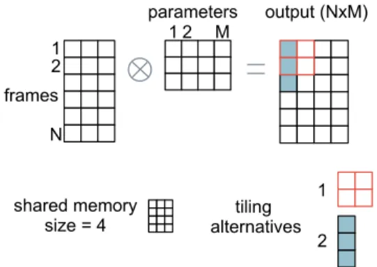
Shared Memory Tiling. As discussed in the description of the frame fan-out in §4.1, when audio processing pipelines work on a frame they usually produce multiple output values (e.g., feature co-efficients or probability scores) by combining the frame data with multiple parameters. The procedure can be treated asgeneralized dense matrix-matrix multiplicationwith the two matrices being: 1) an input matrixI(n,d) withninput frames each of which has d elements (samples/coefficients); and 2) a parameter matrixP(k,d) withk parameters each of which has dimensionalityd. The re-sult of the combination of the two matrices is a matrixO(n,k) = I(n,d)NP(Tk,d)where

N

can be a generalized operation that per-forms a reduction overdelements from the two matrices (a row fromOand a column fromPT_{). Prominent applications of this}

operation can be found in the computation of the filter bank co-efficients, the GMM mixture probability estimation, and the DNN

tiling alternatives shared memory size = 4 frames 1 N 2 parameters 1 2 M output (NxM) 1 2

Figure 5: Tiling example. There are N frame data rows and M parameter columns that can be combined to yield N×M output val-ues. The shared memory size of a work group is limited to4frame rows or parameter columns in total. There are2tiling alternatives. Alternative1fills shared memory by loading data for2frames and

2parameters leading to4computed values in total from the work group. Alternative2loads data for3frames and1parameter lead-ing to3computed values in total.

network propagation. An example reductionN

used in the GMM classification stage is shown in the following equation:

oij=− 1 2(gj+ X 0≤s<d (xis−mjs)2vjs) (1)

whereoijis one element from the output matrix;mj,vj, andgj

are the Gaussian parameters of a mixture component; andxiare

feature values from framei.

The straightforward implementation of a GPU kernel to compute matrixOwould be to let each thread compute one output valueoij

and load independently an input rowiand a parameter columnj. However, a strategy for reducing global memory traffic is to intro-duce a model-specific version oftiled algorithmsused in matrix-matrix multiplication [40]. The core idea is to let the work groups of a kernel partition the output matrix intotilesso that the total data for each tile fits into shared memory. Our goal is to have the threads in a work group collaboratively load both input data and parame-ters into shared memory in a way that maximizes the number of computations per global memory read. This can be achieved if the number of computed values ({number of frames}Nf ×{number

of parameters}Np) per loaded data is as large as possible for the

entire work group. Figure 5 illustrates the pattern in operation.

4.3

Parameter Estimation

We calculate key optimization parameters as described below. Vector sizex. The engine selects the vector size for batched mem-ory reads by querying with OpenCL commands whether the audio kernel can successfully be compiled with the given value forx. The engine enumerates the possible values forxin descending or-der and picks the highest value unor-der which the kernel successfully compiles. Compilation may fail when the size of the vectorized loads exhausts the thread register space.

Memory slidingκ. Optimizing this parameter involves solving a linear equation with respect to the GPU shared memory size, and input model parameters. IfSM is the total number of values the

shared memory can accommodate,SF is the input region size, and

ris the frame offset in number of input values, then the maximum κis computed in the following manner:κ=jSM−SF

r k

+ 1. Memory tilingκ. The optimization engine makes a two-staged

decision: whether to activate this pattern and if activated how to best parameterize it. The decision is based on the type of the model used for audio analysis (filter banks, GMM, or DNN), input model dimensions (size of the model parameters), maximum work group size, and shared memory size. The optimization engine estimates the work group size and an optimum number of output matrix val-ues each thread in the work group should compute so that global memory accesses are minimized. This is implemented by solving a quadratic equation with respect toNf andNpunder the shared

memory constraints. In our examples, the pattern would be acti-vated for the filter banks and GMM computation, but not for the DNN where the size of the network is prohibitively large for any meaningful subset to be effectively exploited from shared memory. Frame fan-outφand work group size. The engine estimates the fan-out factor in a final step by reading the specified audio model parameters (e.g., number of frames) and havingκdetermined in a prior step. We strive to select the largest work group size possible. Similarly to vectorization, this can be done by exhaustively trying to compile the kernels with values up to the maximum size allowed. Sizes are enumerated in multiples of thepreferred group multiple parameter(queried from the GPU with OpenCL).

5.

IMPLEMENTATION

We briefly summarize the details of the software artifacts used in this work.

Hardware and APIs. We prototype the audio sensing algorithms on a Snapdragon 800 Mobile Development Platform for Smart-phones (MDP) [16] with an Android4.3Jelly Bean OS featuring Adreno 330 GPU present in mobile phones such Samsung Galaxy S5 and LG G Pro2. All GPGPU development is done with OpenCL 1.1 Embedded Profile and we reuse utilities for initializing and querying the GPU from the Adreno SDK that is openly available [13]. In addition, we prototype baseline versions of the audio sens-ing pipelines for the Qualcomm Hexagon DSP [14] with the Hexagon C SDK v1.0 [15]. The DSP has3hardware threads and we use thedspCVthread pool library shipped with the Hexgagon SDK to build multithreaded versions of the algorithms for the DSP. The CPU sequential baselines reuse the C code built for the DSP and are accessed by interfacing with the Android Native Development Kit (NDK). Multithreaded CPU versions are built by using C++11 threads – we leverage the4cores available to the Snapdragon Krait CPU. Note, our implementation does not explicitly leverage, nor is structured for the use of, SIMD instructions (like NEON) as avail-able in the Krait CPU. Although we take advantage of Qualcomm SDK primitives and other best practices (described next) that en-hance the performance of the CPU and DSP in the Snapdragon. Power measurements are performed with a Monsoon Power Mon-itor [8] attached to the MDP. Classifier models are trained with the HTK toolkit [6] for the Speaker/Emotion Recognition and the Theano python library [18] for the Keyword Spotting.

DSP Baseline Implementation.We implement basic DSP bench-marks as a ballpark reference on energy consumption and a first indication of latency when machine learning algorithms found in audio sensing are executed on a low-power chip. As stated above, we use the Qualcomm Hexagon SDK to tailor implementations to the DSP which are not a direct compilation of CPU-based code. The DSP C language features are a subset of the standard C distri-butions [28], which is why without significant modifications most CPU algorithms cannot be directly executed on the Hexagon DSP. Instead, we build our baselines to match the requirements and con-ventions of the Hexagon Elite SDK for audio processing, our

ba-sis is DSP-targeted code which has been modified to be executed on the CPU as well. Although we have yet to take advantage of the more advanced VLIW (Very Long Instruction Word) instruc-tions available to the DSP everywhere in our code, our DSP im-plementations are not naive CPU-variants as we reuse some of the optimized DSP processing routines coming readily with the DSP SDK (such as FFT computation): these already come with VLIW optimized instructions and intrinsics. The algorithms that are not included in these DSP libraries we have implemented ourselves fol-lowing the guidelines provided by the Elite audio processing SDK (e.g., for memory allocation). We acknowledge additional research is needed to find the most optimal DSP implementations, however we do leverage optimized algorithmic primitives distributed with the SDK to give some reference numbers on the amount of en-ergy required to process machine learning algorithms found in au-dio sensing.

Kernel Compilation. Building the OpenCL kernels can be done either via reading the sources from a string and compiling them at runtime or by compiling the source into a binary. We use pre-compiled binaries that drastically reduce the kernel load time and that need to be produced once per deployment.

6.

EVALUATION

In this section, we provide an extensive evaluation of the parallel optimizations under representative audio sensing algorithms when deployed on a mobile GPU. The main findings are:

• Optimizing the control-flow parameters is critical – naively pa-rameterized GPU implementations may be up to 1.5x slower than multithreaded CPU baselines and consume more than2x the energy of offloading batched computation to the cloud.

• The total speedup against a sequential CPU implementation for an optimized GMM-based and a DNN-based pipeline running entirely on the GPU is8.2x and13.5x respectively, making the GPU the processing unit of choice for fast real-time feedback. The optimized GPU is also3-4x more energy efficient than se-quential CPU implementations, but can consume up to3.2x more energy than a low-power DSP.

• After a certain batching threshold (10to 20seconds) of com-puting multiple inferences in one go, optimized GPU algorithms begin to consume less energy than cloud offloading with good throughput (5Mbps and10Mbps), in addition to obtaining infer-ences3.1x and6.5x times faster for the GMM and DNN-based pipelines respectively.

• The total energy consumption under batching scenarios is in ranges comparable to those delivered by reference low-power DSP im-plementations with some basic optimization.

6.1

Experimental Setup

Experiments are performed with the display off and the algo-rithms are executing in the background, as is typical for sensing apps to operate in such mode. We denote withAudio Optimized GPU (a-GPU)the output from the optimization engine as described in §3. Throughout the section we use the following baselines.

• DSP sequential (DSP). Our DSP baselines are implemented as specified in Section 5 via the Hexagon DSP in DSP- com-patible C. We reuse optimized built-in primitives for FFT computation, memory allocation and follow the conventions of the Elite SDK for audio processing. Our implementations are meant to be used as a ballpark reference on the energy efficiency that can be supported by low-power units but do

not claim they are the most efficient that can be achieved through advanced hardware optimizations applied rigorously throughout the code base.

• CPU sequential (CPU). Our implementations have a sequen-tial workflow that follows the DSP code structure but reim-plements some of the routines that require DSP-specific VLIW instructions (e.g., FFT computation). The baselines are based on DSP-compatible C.

• CPU multi-threaded (CPU-m). We implement variants of the pipeline algorithms where the bottleneck classification stage of the audio pipeline (occupying>90%of the runtime in our examples) is parallelized across multiple threads. The GMM classification is restructured so that each GMM model proba-bility is the unit of work for a separate thread. We maintain a pool of4threads which equals the number of physical cores of the Snapdragon Krait CPU – adding more threads did not lead to any performance benefits. The DNN classification is restructured so that the network propagation step is per-formed in parallel: each thread processes the activation of one node in a layer.

• DSP multi-threaded (DSP-m). Similarly to the multi-threaded CPU versions of the algorithms, we adopt DSP alternatives that parallelize the pipeline classification. The parallel DSP variants have logically the same threading model as the CPU one, with the difference that the DSP thread pool size is3, i.e. it equals the number of hardware threads. We use the worker pool utility librarydspCVwhich speeds up the execution for Computer Vision algorithms on the DSP.

• Naive GPU (n-GPU). We add the most naively parameter-ized GPU implementations as explicit baselines in addition to showing different parameter configurations. For all algo-rithmic building blocks (GMM, DNN, and features) in this naive baseline category we set the vectorized load factorx= 1, and the per-frame compute factor to beκ=νwhich re-sults in a frame fan-out factor ofφ=n.

Energy Measurements. All energy measurements are taken with a Monsoon Power Monitor attached to our MDP device. By de-fault, the experiments were performed with a display off, with no services running in the background except system processes. This reflects the case when GPU offloading is done in the background, as in a continuous sensing scenario. The power evaluation setup closely matches the one reported by LEO [29]. Each application is profiled separately for energy consumption by averaging power over multiple runs on the CPU, DSP and GPU.

6.2

Pattern Optimization Benchmarks

In this subsection, we study how the application and parame-terization of the various optimization techniques presented in §4 affect the GPU kernel runtime performance. Table 4 shows differ-ent points in the parameter space compared to the engine optimized configuration.

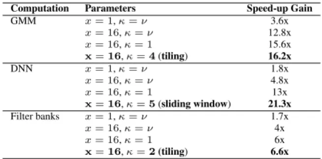
Pattern Speedups. A first observation is that using vectorization with larger batches (x= 16) provides a significant boost across all algorithms. The speedup of the most naïve GMM kernels jumps from 3.6x to 12.8x, the DNN ones – from 1.8x to4.8, and the filter banks – from1.7x to4x. The success of this simple technique can be attributed to the fact that the mobile GPU is optimized to efficiently access multiple items with a single instruction.

Another observation is that increasing the fan-out factorφby settingκ = 1provides tangible runtime boosts. As illustrated,

Computation Parameters Speed-up Gain GMM x= 1,κ=ν 3.6x x= 16,κ=ν 12.8x x= 16,κ= 1 15.6x x=16,κ=4(tiling) 16.2x DNN x= 1,κ=ν 1.8x x= 16,κ=ν 4.8x x= 16,κ= 1 13x x=16,κ=5(sliding window) 21.3x Filter banks x= 1,κ=ν 1.7x x= 16,κ=ν 4x x= 16,κ= 1 6x x=16,κ=2(tiling) 6.6x

Table 4: Parameter configuration speed-ups vs. CPU sequential implementation. Lines in bold show the optimal parameter values found by the optimization engine.

speedups increase from12.8x to 15.6x for the GMM, and from

4.8x to 13x for the DNN. Interestingly, the higher fan-out pro-vides benefits even though the number of global memory accesses is raised by issuing writes of intermediate values to a scratch mem-ory. The reason for this is that the fan-out pattern prominently in-creases the total number of work items and as a consequence there are more opportunities for the GPU to hide memory access laten-cies – whenever a group of threads is stalled on a memory read or write operation, with a higher probability the GPU can find another group that can perform computation while the former waits.

Last but not least, the more advanced tiling and sliding win-dow techniques tuned by the optimization engine provide notice-able speedup improvements over the straightforward use of shared memory. The sliding window optimization boosts the second best DNN kernel speedup from13x to21.3x, which is also the highest cumulative gain observed across all algorithms. Optimally param-eterized tiling, on the other hand, brings the overall GMM speedup to16.2x and filter banks to6.6x. In these cases, increasingκ fur-ther results in suboptimal use of shared memory – since its size is limited, the work items can fetch only a proportion of the total data they need, the rest needs to be loaded from the slower global memory into thread registers.

Summary. The engine optimized kernels allow GPU computa-tion to exhibit much higher performance than naively parameter-ized baselines. The optimization techniques can be ubiquitously applied across multiple stages of the pipelines.

6.3

GPU Pipeline Runtime and Energy

We compare our engine optimized GPU pipelines against the baselines listed in §6.1. Table 5 shows the runtime for running the pipelines on the various processing units. The most prominent observation is that the optimized GPU implementation is the fastest one. For instance, the full GMM and DNN pipelines are8.2x and

13.5x times faster than a sequential CPU implementation respec-tively, an order of magnitude faster. In comparison, the CPU multi-threaded alternatives are around3x times faster only. If the GPU is not carefully utilized, the naively parameterized GPU implemen-tations may be up to1.5x slower than the multicore variants (e.g., DNN pipeline). The reason why the audio-optimized GPU fares so much better than both multicore CPU and naive GPU alternatives is because massive data parallelism is enabled by the parallel tech-niques – the hundreds of cores on the GPU can work on multiple small independent tasks simultaneously and hide memory access latency. This is especially true for the classification tasks that are

16.2x (GMM) and21.3x (DNN) faster than their sequential CPU counterparts.

In Figure 6 we plot the energy needed by the various units to

ex-10 20 30 40 50 Batch Size (seconds) 0 5 10 15 20 25 Energy (J) (a)GMM pipeline 1 2 3 4 5 6 7 8 9 10 Batch Size (seconds) 0 2 4 6 8 10 12 14 Energy (J) n-GPU a-GPU CPU DSP CPU-m DSP-m (b)DNN pipeline

Figure 6: Energy (J) as a function of the audio processing batch size in seconds. Legend is shared, axis scales are different.

ecute the pipeline logic repeatedly on batched audio data. For one-off computations the cheapest alternative energy-wise is the DSP which can be up to3.2x more energy efficient than the optimized a-GPUfor the DNN pipeline. Yet, the a-GPU is between3x and

4x times more energy efficient than the sequential CPU for both applications. If high performance is of utmost priority for an ap-plication, the GPU is the method of choice for on-device real-time feedback– when optimized, GPU offloading will obtain inferences much faster and significantly reduce energy compared to the CPU. A notable observation is that as the size of the buffered audio data increases, the a-GPU begins to deliver energy efficiency in the ranges provided by the low-power DSP. For instance, with batch sizes of10and6seconds for the GMM and DNN pipeline respec-tively, the a-GPU provides comparable energy while being multiple times faster (>50x compared to our reference baselines). If appli-cations can tolerate small delays in obtaining inferences, batched GPU computation will save amounts of energy similarly to a low-power DSP and at the same time obtain results faster. We note that a heavily optimized DSP implementation will be the best option energy-wise; here we show that contrary to conventional wisdom, there is a scenario in which the GPU can be used to save energy on a scale that is much closer to what a low-power unit can achieve.

6.4

GPU Sensing vs Cloud Offloading

Cloud baselines. We compare the performance of the sensing algo-rithms on the GPU against the best performing cloud alternatives. For the DNN-style Keyword Spotting application, the cheapest al-ternative is to send the raw data directly for processing to the cloud because the application generates as many features as the size of the raw input data. For the GMM-style Speaker Identification pipeline, the cheapest alternative is to compute the features on the DSP and send them for classification to the cloud. However, this variant is >10times slower than computing the features on the CPU. Fur-ther, we find that when sending the features to the cloud, establish-ing the connection and transferrestablish-ing the data dominate the energy needed to compute features on the CPU. For this reason, the GMM cloud baseline in our experiments computes features on the CPU and sends them for classification to a remote server.

Latency Results. In Figure 7 we plot the end-to-end time needed to offload one pipeline computation to the cloud and compare it against the total time required by the GPU to do the processing (including the GPU kernel set-up and memory transfers). We as-sume a window size of64KB and vary the network RTT so that the throughput ranges from1to20Mbps. Given this, the a-GPU imple-mentation is3.1x and6.5x faster than the good5Mbps cloud alter-native for the GMM and DNN pipelines respectively. This comes at

GMM full pipeline GMM classification DNN full pipeline DNN classification DSP -8.8x -8.6x -4.5x -4.0x DSP-m -3.2x 2.5x -2.1x -1.5x CPU (runtime) 1.0x (1573 ms) 1.0x (1472 ms) 1.0x (501 ms) 1.0x (490 ms) CPU-m 3.0x 3.4x 2.8x 2.9x n-GPU 3.1x 3.6x 1.8x 1.8x a-GPU 8.2x 16.2x 13.5x 21.3x

Table 5: Speedup factors for one run of the various pipeline implementations compared against the sequential CPU baseline. Negative numbers for the DSP variants show that the runtime is that amount of time slower than the CPU baseline. CPU average runtime in ms is given for reference in brackets. Note that the DSP numbers are provided by our reference implementation under the conditions specified in the baseline definition. A highly optimized DSP implementation might challenge the CPU latency-wise in certain scenarios. We still expect the a-GPU to be the lead given its current massive speed-ups.

1 5 10 20 n- a-0.0 0.4 0.8 1.2 1.6 Runtime (s) (a)GMM 1 5 10 20 n- a-0.0 0.4 0.8 1.2 1.6 Runtime (s) (b)DNN

Figure 7: End-to-end latency for computing the audio pipelines on the GPU vs cloud. Numbers on the x axis show throughput in Mbps, and n- and a- refer to n-GPU and a-GPU.

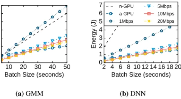
10 20 30 40 50 Batch Size (seconds) 0 1 2 3 4 5 6 7 Energy (J) (a)GMM 2 4 6 8 10 12 14 16 18 20 Batch Size (seconds) 0 1 2 3 4 5 6 7 Energy (J) n-GPU a-GPU 1Mbps 5Mbps 10Mbps 20Mbps (b)DNN

Figure 8: End-to-end energy as a function of the batch compu-tation size for running the audio pipelines on the GPU vs cloud offloading. Legend is shared.

the expense of a1.6x and1.4x increase in the energy for a one-off computation for the two pipeline types respectively. The takeaway is thatif speed is favoured over energy, the GPU should be used for local processing because it will deliver inference results several times faster than cloud offloading even with good connectivity. Energy Results. In Figure 8 we plot the total energy required to offload batched pipeline computations to the cloud as a function of the batch size in seconds for which raw audio data is queued for processing. The most notable outcome is thatthe a-GPU com-petes energy-wise with good connectivity cloud offloading in addi-tion to being multiple times faster. After a certain batching thresh-old, the total processing with the optimized a-GPU consumes even less energy. For instance, unless the network has a throughput of

20Mbps (and an RTT of25ms) the GMM-style pipeline starts get-ting cheaper than the faster connections after20seconds of buffered audio, and the DNN Keyword Spotting pipeline – after only10

seconds of audio data. The reason for this phenomenon (batched processing is less expensive than cloud and one-off computation is not) is that the initial kernel set-up and memory transfer costs are

GMM DNN 0.0 0.2 0.4 0.6 0.8 1.0 Energy (J) GMM cloud DNN cloud

Figure 9: Energy consumed for one-off computation for the GMM- and DNN-based audio apps. Lighter shaded bars show en-ergy spent for processing, the rest is GPU tail enen-ergy. Lines show the total energy consumed by cloud offloading for the two apps for a network connection with an RTT of104ms.

high, but once paid, the a-GPU offers better energy per second for audio sensing.

In Figure 9 we plot a breakdown of the energy for a one-time run of the audio apps on the GPU to quantify the GPU setup over-head. Overall, the amount of energy spent in the GPU tail states is over65% of the total consumption for both applications which confirms the prohibitively high setup/tear-down GPU costs. With a network that has an average RTT of104ms (translating to≈5Mbps throughput), the energy spent by cloud offloading is less than the GPU setup cost. Unless the audio app is highly sensitive to the run-time, cloud offloading may provide a desirable trade-off between energy and latency.

Another critical result is that optimizing GPU execution is cru-cial – the naive n-GPU is more expensive (>2x) energy-wise than almost all types of cloud offloading when batching. With the bet-ter but still unoptimized baselines with highest fan-out (κ = 1), the batching threshold for preferring GPU execution over cloud is higher (e.g.,≈14seconds for the DNN algorithm), delaying the application response time further than what could be achieved with the engine optimized version.

Summary. While cloud offloading has a significant computational lead over mobile, the GPU now provides advantages that makes local processing highly desirable – it is faster, less susceptible to privacy leaks as execution is entirely local, works regardless of con-nection speed, and even competes with cloud in terms of energy.

6.5

GPGPU and Graphics Workloads

Here we investigate how GPGPU computations interfere with other GPU workloads such as those used for graphics processing – will the background GPU computation affect negatively the user ex-perience?We schedule the execution of the audio sensing pipelines (either Speaker Identification or Keyword Spotting) to run

continu-AB FN CR ABG SS 0 20 40 60 80 Average FPS no GPGPU load with GPGPU load

(a)Frame rate (FPS)

AB FN CR ABG SS 0 20 40 60 80 100 GPU load (%)

(b)total GPU load

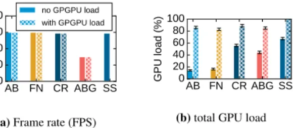
Figure 10:Average frame rate and GPU load when the games run without and with additional GPGPU load. Games in the experiment are Angry Birds (AB), Fruit Ninja (FN), Crossy Road (CR), Angry Birds GO (ABG), and Subway Surfers (SS). Legend is shared.

ously for a minute on the GPU while the mobile user is interacting with other applications that are known to strain the GPU resources, i.e. games. We pick5hugely popular Android games with multi-million downloads and different play styles (Angry Birds, Fruit Ninja, Crossy Road, Angry Birds GO, and Subway Surfers), and observe the effect GPGPU computation has on the perceived game-play quality. To quantify this we measure the average frame rate (frames per second (FPS)) with GameBench [3] during gameplay over5 1-minute long runs.

In Figure 10 we show the aggregate results from the experi-ments. For all games except Subway Surfers the GPGPU com-putation does not change the original frame rates of the games, although the total GPU load substantially increases. For instance, the render-heavy racing Angry Birds GO maintains an average frame rate of30FPS both with and without the added audio sensing work-load, even though the total GPU load jumps from44% to85%. For this and the other three games with similar behavior (Angry Birds, Fruit Ninja, Crossy Road), the effect can be explained by the facts that 1) the original load the games place on the GPU is not too high, 2) GPU rendering is time-shared with GPGPU computation, and 3) the audio sensing kernels are short-duration (a single kernel execu-tion never exceeds tens of milliseconds). With the endless runner Subway Surfers, however, the original average GPU load is already very high (≈70%), and adding the GPGPU computation results in a screen freeze so that the game becomes unresponsive. This can be attributed to the fact that the OS does not treat the GPU as a shared resource and there is a lack of isolation of the various GPU work-loads. One way to approach this is introduce OS-level abstractions that provide performance guarantees [51].

7.

DISCUSSION AND IMPLICATIONS

Here we survey key scenarios and issues related to the applica-bility of the GPU parallel optimizations for audio sensing. Targeted Scenarios. There are many chains of audio workloads that we envisage are relevant to GPU offloading with delayed cloud-free batch processing. Examples are continuous low latency audio tasks (hot key word recognition) followed by a much heavier pro-cessing that is more tolerant to the delays offered by GPU acceler-ation – all types of analysis possible on human voice fall into this category. There are numerous such examples of behavior moni-toring in the audio sensing literature: conversation analysis [46], speaker counting [56], speaker identification [43], emotion recog-nition [50], and ambient scene analysis [45] to name a few. Context monitoring through sounds and triggering notifications (e.g., detect conversation to mute the speaker) is another key functionality that can be supported with this type of offloading: delayed cloud-free batch processing with entirely offline trained models, or models

that need to be only infrequently updated. GPU offloading will be a crucial part of more complicated scheduling schemes that involve other processing units as well (e.g., [29]) and possibly cloud. In that case hybrid solutions that use multiple processing units and cloud can reap the benefits of GPU execution, and more applica-tions including those that need cloud support such as Shazam can take advantage of the more advanced local processing (e.g., to ex-tract the features necessary to discriminate the encountered songs).

7.1

Implications

We believe the results presented in this work provide insights of value to the following areas.

Privacy. Our findings suggest that algorithms optimized for embed-ded-class GPUs can bring the much coveted privacy guarantees to devices such as Amazon Echo [1] and Google Home [4], if the operation remains entirely on the device itself. These assistants re-spond to simple home user requests (such as, “turn on the light”), but are known to heavily exploit cloud offloading. With the help of our techniques doing the processing locally on the GPU can be done faster than cloud offloading, and without exposing sensitive information to untrusted third parties.

Servicing multi-app workloads. GPUs will play a crucial role in offloading the sensing workloads of digital assistants as they can-not be serviced by the DSP capabilities alone. Amazon Echo, for instance, performs multiple audio sensing tasks on a continuously processed audio stream, including: 1) detect the presence of speech vs other sounds; 2) perform spoken keyword spotting (as all com-mands are triggered by the same starting word); and, 3) speech recognition, along with additional dialog system analysis that al-lows it to understand and react to the command. These tasks col-lectively are well beyond the DSP processing and memory capabil-ities [28], in such multi-app audio sensing scenarios approaching the mobile GPU with routines that maximize runtime performance and minimize energy consumption is critical.

Energy reductions. Audio sensing algorithms are notorious for their continuous monitoring of the sensor stream. Whereas DSP offloading is massively adopted as the go-to power reduction ap-proach for applications such as hot keyword spotting, with the in-crease in number of concurrent audio sensing services mobile users adopt (e.g., Google Now, Auto Shazam), the DSP will have to se-lectively process a subset of the algorithm stages. In multi-app scenarios, optimally using the GPU as we have done in this work will be instrumental in keeping the power-hungry CPU or privacy-invading cloud offloading at bay.

7.2

Discussion

Our design, and its results, also highlight the following issues. Performance on other mobile GPU varieties.Although it is highly likely there will be a difference in the exact values for the perfor-mance boosts on other GPU models (such as NVIDIA’s Tegra), we expect qualitatively similar results when deploying the pipelines there. For example, speedups from the GPU data parallelism will be sufficiently high to deliver real-time performance for applica-tions that can afford the energy costs. This is because our proposed optimizations can be generalized to any OpenCL-compliant GPU architecture, and do not rely on vendor-specific features.

Parallelizing other sensor processing algorithms.The core me-chanics behind the optimization patterns can be applied to other classifiers such as Support Vector Machines (SVM), and deep learn-ing network topologies such as Convolutional Neural Networks (CNN). This is because the patterns depend on how the

classifica-tion is applied to the audio data stream (in sliding windows, com-bining model parameters with frame data independently to different frame offsets), rather than fully depend on the concrete algorithm implementation. We believe the broader lessons learned from this work on using the GPU will promote further research into how it can be used to accelerate algorithms in other application domains (e.g., alternative sensor processing from accelerometer, or GPS). GPU vs. multicore CPUs. As single-thread performance for mi-croprocessor technology is leveling off, multiple cores will become major drivers for increased performance [20] (e.g., up to61for Intel Xeon Phi [7]). Developers will likely be faced with similar data parallel challenges – increasing the total number of concur-rent tasks for better utilization, and efficiently leveraging memory caches to mask access latency. As OpenCL manages heteroge-neous parallel algorithms transparently from the underlying mul-ticore architecture, the developed OpenCL-compliant optimization techniques will prove valuable to multicore CPUs as well. GPU programmability.GPUs are notoriously difficult to program – even if the algorithm exhibits data parallelism, restructuring it to benefit from GPU computation often requires in-depth knowledge about the algorithm mechanics. In fact, automated conversion of sequential to parallel code has been an active area of research [22, 21], but fully automating the parallelization process still remains a big challenge. We provide a portable OpenCL library of parallel implementations for key audio sensing algorithms (e.g., GMMs, DNNs) and expect developers will either compose pipelines by reusing the OpenCL host and kernel code, or by applying the in-sights from our optimization patterns to their implementations.

We acknowledge that currently programming GPUs requires skill-ful development. We hope that through our library we can simplify the pure GPU kernel development by providing optimized machine learning primitives developers can reuse. Without them, develop-ers will mostly likely encounter the problems we uncovered while designing our library (e.g., memory-bound processing) in order to incorporate GPU processing into their audio application. We do not fully automate the process, a potential direction for future research is designing or reusing a simpler high-level declarative language that can be used to specify pipeline processing. In the case that all algorithmic components are covered by our library, this can greatly simplify the developer burden. This compiler component can be built on top of CUDA/OpenCL or industrial strength GPU APIs.

8.

RELATED WORK

Our work is touches most closely the following areas of research related to efficient sensing and efforts to optimize GPU usage. Sensor Processing Acceleration and Efficiency. A large body of research has been devoted to the use of heterogeneous computation via low-power co-processors [49, 43, 28,?,?, 52] and custom-built peripheral devices [54] to accelerate or sustain power efficient pro-cessing for extended periods of time. Little Rock [49] and Speak-erSense [43] are among the first to propose the offloading of sensor sampling and early stages of audio sensing pipelines to low-power co-processors – the processing enabled by such early units is ex-tremely energy efficient but limited by their compute capabilities to relatively simple tasks such as feature extraction. DSP.Ear [28] and Shen et al. [52] study more complex inference algorithms for continuous operation on DSPs but demonstrate such units can be easily overwhelmed and often the energy efficiency comes at the price of increased inference latency.

LEO [29] is a low-power scheduler that dynamically distributes computation across heterogeneous resources, including the GPU

as a possible resource, and lowers the overall energy consumption for concurrent sensor apps. However, it does not investigate the trade-offs of GPU offloading in detail, nor does it show what is required to optimally utilize such a processing unit. We believe the optimizations we designed complement sensor scheduling, and are critically needed to allow frameworks to maximize GPU usage. General-Purpose GPU Computing. GPUs have been used as general-purpose accelerators for a range of tasks, the most popu-lar applications being computer vision [55, 24, 37] and image pro-cessing [53, 48]. Object removal [55] and face recognition [24] on mobile GPUs have been showcased to offer massive speedups via a set of carefully selected optimization techniques. Although the techniques found in the graphics community as well as in the field of speech processing (fast spoken query detection [58]) ad-dress similar data parallel challenges to what we identify (increas-ing thread throughput, careful memory management), these tech-niques remain specific to the presented use cases.

The GPU implementation of automatic speech recognition based on GMMs [30], for example, proposes optimizations that are re-lated to the specifics of a more complex speech recognition pipeline. Instead, we target a different workload scenario emerging from a growing number of coarse-sound classification applications that require processing that can happen entirely cloud-free. For this distinctly different workload, we introduce general techniques that are applied at the level of the machine learning model, or the level of organization related to multiple algorithms for processing audio data. As such, the insights drawn from our work are directly appli-cable to a class of algorithms that build upon commonly adopted machine learning models in audio sensing.

Packet routing [32] and SSL encryption [38] leverage GPUs to increase processing throughput via batching of computations, but none of these works is focused on studying energy efficiency as-pects which are critical for battery-powered devices.

GPU Resource Management. PTask [51] is an OS-level abstrac-tion that attempts to introduce system-level guarantees such as fair-ness and performance isolation, since GPUs are not treated as a shared system resource and concurrent workloads interfere with each other. The relative difficulty in manually expressing algo-rithms in a data parallel manner may lead to missed optimization opportunities – works such as those of Zhang et al. [57] and Jog et al. [39] attempt to streamline the optimization process. The former improves GPU memory utilization and control flow by au-tomatically removing data access irregularities, whereas the lat-ter addresses problems with memory access latency at the thread scheduling level. Both types of optimizations are complementary to our work – we optimize the general structure of the parallel audio processing algorithms, while the mentioned frameworks tune par-allel behavior of already built implementations. Last but not least, Sponge [36] provides a compiler framework that builds portable CUDA programs from a high-level streaming language. Instead, we study the trade-offs mobile GPUs provide for sensing, and build on top of OpenCL which together with the Qualcomm Adreno GPU dominates the mobile market.

9.

CONCLUSION

In this paper we have studied the trade-offs of using a mobile GPU for audio sensing. We devised an optimization engine that leverages a set of structural and memory access parallel patterns to auto-tune GPU audio pipelines – optimized GPU routines are an or-der of magnitude faster than sequential CPU implementations, and up to6.5x faster than cloud offloading (5Mbps throughput). With just10-20seconds of batched audio data, the optimized GPU

be-gins to consume less energy than cloud offloading and in the range typical for low-power DSPs. The insights drawn can help towards the growth of the next-generation mobile sensing apps that leverage GPU capabilities for extreme runtime and energy performance.

10.

ACKNOWLEDGMENTS

This work was supported by Microsoft Research through its PhD Scholarship Program. We thank the anonymous reviewers and our shepherd (Lin Zhong) for their valued comments and suggestions.

11.

REFERENCES

[1] Amazon Echo. http://www.amazon.com/

Amazon-Echo-Bluetooth-Speaker-with-WiFi-Alexa/dp/ B00X4WHP5E.

[2] Apple Siri. https://www.apple.com/uk/ios/siri/. [3] GameBench. https://www.gamebench.net/. [4] Google Home. https://home.google.com/.

[5] Google Now. http://www.google.co.uk/landing/now/. [6] HTK Speech Recognition Toolkit. http://htk.eng.cam.ac.uk/. [7] Intel Xeon Phi. http://www.intel.com/content/www/us/en/

processors/xeon/xeon-phi-detail.html. [8] Monsoon Power Monitor.

http://www.msoon.com/LabEquipment/PowerMonitor/. [9] NVIDIA CUDA. http://www.nvidia.com/object/cuda_home_new.html. [10] NVidia Tegra X1. http://www.nvidia.com/object/tegra-x1-processor.html. [11] OpenCL. https://www.khronos.org/opencl/.

[12] Qualcomm Adreno GPU. https:

//developer.qualcomm.com/software/adreno-gpu-sdk/gpu. [13] Qualcomm Hexagon DSP. https://developer.qualcomm.com/mobile-development/ maximize-hardware/multimedia-optimization-hexagon-sdk/ hexagon-dsp-processor. [14] Qualcomm Hexagon SDK. https://developer.qualcomm.com/mobile-development/ maximize-hardware/multimedia-optimization-hexagon-sdk. [15] Qualcomm Snapdragon 800 MDP. http://goo.gl/ySfCFl. [16] TensorFlow. https://www.tensorflow.org/.

[17] Theano. http://deeplearning.net/software/theano/. [18] C. M. Bishop.Pattern Recognition and Machine Learning

(Information Science and Statistics). Springer-Verlag New York, Inc., Secaucus, NJ, USA, 2006.

[19] S. Borkar and A. A. Chien. The future of microprocessors. Commun. ACM, 54(5):67–77, May 2011.

[20] S. Campanoni, K. Brownell, S. Kanev, T. M. Jones, G.-Y. Wei, and D. Brooks. Helix-rc: An architecture-compiler co-design for automatic parallelization of irregular programs. InProceeding of the 41st Annual International Symposium on Computer Architecuture, ISCA ’14, pages 217–228, Piscataway, NJ, USA, 2014. IEEE Press.

[21] S. Campanoni, T. M. Jones, G. H. Holloway, G.-Y. Wei, and D. M. Brooks. Helix: Making the extraction of thread-level parallelism mainstream.IEEE Micro, 32(4):8–18, 2012. [22] G. Chen, C. Parada, and G. Heigold. Small-footprint

keyword spotting using deep neural networks. InIEEE International Conference on Acoustics, Speech, and Signal Processing, ICASSP’14, 2014.

[23] K. T. Cheng and Y. C. Wang. Using mobile gpu for general-purpose computing – a case study of face recognition on smartphones. InVLSI Design, Automation

and Test (VLSI-DAT), 2011 International Symposium on, pages 1–4, April 2011.

[24] D. Chu, N. D. Lane, T. T.-T. Lai, C. Pang, X. Meng, Q. Guo, F. Li, and F. Zhao. Balancing energy, latency and accuracy for mobile sensor data classification. InProceedings of the 9th ACM Conference on Embedded Networked Sensor Systems, SenSys ’11, pages 54–67, New York, NY, USA, 2011. ACM.

[25] A. de Cheveigné and H. Kawahara. YIN, a fundamental frequency estimator for speech and music.The Journal of the Acoustical Society of America, 111(4):1917–1930, 2002. [26] Z. Fang, Z. Guoliang, and S. Zhanjiang. Comparison of

different implementations of mfcc.J. Comput. Sci. Technol., 16(6):582–589, Nov. 2001.

[27] P. Georgiev, N. D. Lane, K. K. Rachuri, and C. Mascolo. DSP.Ear: leveraging co-processor support for continuous audio sensing on smartphones. InProceedings of the 12th ACM Conference on Embedded Network Sensor Systems, SenSys ’14, New York, NY, USA, 2014. ACM.

[28] P. Georgiev, N. D. Lane, K. K. Rachuri, and C. Mascolo. Leo: Scheduling sensor inference algorithms across heterogeneous mobile processors and network resources. In Proceedings of the 22Nd Annual International Conference on Mobile Computing and Networking, MobiCom ’16, pages 320–333, New York, NY, USA, 2016. ACM.

[29] K. Gupta and J. D. Owens. Compute & memory

optimizations for high-quality speech recognition on low-end gpu processors. InProceedings of the 2011 18th

International Conference on High Performance Computing, HIPC ’11, pages 1–10, Washington, DC, USA, 2011. IEEE Computer Society.

[30] K. Han, D. Yu, and I. Tashev. Spee