/36
Binary Classification
Using Fast Gaussian
Filtering Algorithm
Kentaro Imajo, Keisuke Otaki,
Akihiro Yamamoto (Kyoto University)
December 1, ALSIP 2012
Abstract
Speed up binary classification on 2D/3D
using the Gaussian kernel
faster than C-SVMs if # of data is 150,000+. Training (pre-computation):
O(n3) → O(4dnlog2dn)
Prediction:
/36
Existing Work
C-SVM is a good binary classifier, but – learning takes O(n3) time,
– prediction takes O(n) time.
We cannot use C-SVMs if # of data gets large.
December 1, ALSIP 2012
3
Solution
Training: O(n3) → We don t learn.
But it takes O(4dnlog2dn) for pre-computation.
Treat every datum equally.
– For future works,
we want to pretend learning of C-SVM, though.
Prediction: O(n) → O(4dlog2dn)
Speed it up
/36
Outline
1. Fast Gaussian filtering algorithm (FGFA)
– A fundamental algorithm of this study 2. Binary classification using FGFA
– Extension of the previous work for binary classification
3. Evaluations 4. Conclusions
December 1, ALSIP 2012
5
1. Fast Gaussian Filtering Algorithm
2. Binary Classification Using
The Fast Gaussian Filtering Algorithm
3. Evaluations
/36 The fast Gaussian filtering algorithm
computes one Gaussian-filtered pixel
in constant time to the area size n (∝ σ2).
The naïve method requires O(n) time.
Benefit of FGFA
December 1, ALSIP 2012
×
Area size is n Target Pixel
7
Key Ideas of FGFA
• The Gaussian function can be
approximated with a spline. • Splines become discrete
if they are differentiated some times.
• Convolution of an image and a spline
would be computed fast
since convolution of an image and a discrete function is easy.
/36
Gaussian Function
The Gaussian filter is computed by
convolutions with the 2D Gaussian function.
The 2D Gaussian Function:
where a parameter σ is variance.
December 1, ALSIP 2012
1
2
exp
x
2+
y
22
2 Circle 9-15 -12.5 -10 -7.5 -5 -2.5 0 2.5 5 7.5 10 12.5 15 80 160 240
˜(
x
) = 3(
x
+ 11)
2+11(
x
+ 3)
2++11(
x
3)
2+3(
x
11)
2+,
2
.
657
10
2exp
5.2720x2 2.
Approximation
×
×
×
×
−
Approximation−
Gaussian func.×
Control points/36
Approximation of 2D
December 1, ALSIP 2012
11
using a discrete image J, which is written as: J(x, y) = !
(∆x,∆y)∈Z2+
∆xn∆ynI(x − ∆x, y − ∆y).
When a source image I is given, the image J can be
computed in O(n2|I|) time by iterations as well as
Equation (6).
As a result, precomputing J at once, for any
convo-lution of a source image I and an nth-order 2D spline
function, a convoluted value ( ˜ψII ∗I)(x, y) can be
com-puted in O(m2) time.
6. Approximated Gaussian Functions
In this section, we present two good sets of param-eters below to approximate the 1D Gaussian function. Absolute values of parameters b of a good set should
be small for easy and fast computation, and absolute values of the parameters b of the following sets are not
larger than 22, which is small, compared with ordinary images. Second-order approximation: ˜ ψ2(x) = 3(x + 11)2+ − 11(x + 3)2+ +11(x − 3)2+ − 3(x − 11)2+, (7) # 2.657 × 10² exp " − x 2 5.27202 # . (8) Fourth-order approximation: ˜ ψ4(x) = 70(x+ 22)4+ − 624(x + 11)4+ +1331(x+ 4)4+ − 1331(x− 4)4+ +624(x − 11)4+ − 70(x − 22)4+, (9) # 7.621 × 10⁷ exp " − x 2 7.767802 # . (10)
6.1. Evaluation of Approximated Functions
Next, we evaluate the approximated functions by cal-culating error of two types EI,ψ˜ and EII,ψ˜, which are
error in 1D and in 2D respectively. Using an approxi-mation function ψ˜ and its targeted function ψ, they are
defined as: EI,ψ˜ = $ R % % %ψ(x) − ψ˜(x)%%%dx $ R ψ(x)dx , (11) EII,ψ˜ = $$ R2 % % %ψ(x)ψ(y) − ψ˜(x) ˜ψ(y)%%%dxdy $$ R2 |ψ(x)ψ(y)|dxdy . (12) 0 10 20 x 0 4×10⁴ 8×10⁴ z · · · Gaussian — Horizontal section - - - Oblique section
Figure 2. Second-order approximation
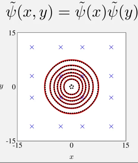
-15 0 15 x -15 0 15 y × × × × × × × × × × × × × × × ×
· · · Gaussian — Approximation × Control point Figure 3. Elevation and control points
Applying the equations, we can calculate values of error of the two approximations (7) and (9), whose tar-geted functions are (8) and (10) respectively, as follows:
EI,ψ˜2 ≈ 0.02009, EII,ψ˜2 ≈ 0.03473,
EI,ψ˜4 ≈ 0.00305, EII,ψ˜4 ≈ 0.00583.
Figure 2 compares the 2D Gaussian function and two sections of the second-order approximated function in two dimension. One of the sections is a horizontal sec-tion z = ˜ψ2(x) ˜ψ2(0), and the other one is an oblique
section z = &ψ˜2(√x2)
'2
.
Figure 3 shows elevations of every 104 for the
Gaus-sian function and the approximation function in two di-mension. As the Gaussian function is rotatable, eleva-tions of the Gaussian function are perfect circles. On the other hand, elevations of the approximated Gaus-sian function, which are indicated by red solid lines, are very similar to perfect circles. Therefore we can use the approximated Gaussian function as an almost-rotatable filter function.
˜(
x, y
) = ˜(
x
) ˜(
y
)
Properties of the Function
• It is a 2nd order spline.
– Piecewise polynomial function
• It has only 2% approximation error
–
• It has only 4 control points
• It has unequal intervals of control points
while general approximation functions often have equal intervals.
– It is sufficiently optimized as a spline.
(
|
˜(
x
)
(
x
)
|
dx
)
/
(
|
(
x
)
|
dx
)
/36
Benefit of Splines
Differentiating splines, they get constant.
The Gaussian-like function can also become discrete!
December 1, ALSIP 2012 13 -12 -8 -4 0 4 8 12 -240 -160 -80 80 160 240 -12 -8 -4 0 4 8 12 -25 25 -12 -8 -4 0 4 8 12 -10 -5 5 10 -12 -8 -4 0 4 8 12 -12 -8 -4 4 8 12 Differentiate 3-times
Speed Up of Convolution
Convolution can be reduced by
differentiating splines
until they become discrete. Intuition:
(
I
)(
x
) =
d
dx
I
(
x
)
dx
(
x
)
Integrated
/36
Transformation
Transform convolution into summation
December 1, ALSIP 2012 15 ( ˜ I)(x) = x Z ˜( x)I(x x) = x Z m i=0 ai( x bi)n+ I(x x) = m i=0 aiJ(x bi), J(x) = x Z xn+I(x x) Pre-computed
O(m) linear combination
The 2D Gaussian function is decomposed:
The approximation can be defined as:
where ( ˜ I)(x, y) = m i=1 ai m j=1 ajJ(x bi, y bj)
2D Convolution
exp x2 + y2 2 2 = exp x2 2 2 exp y2 2 2 O(m2) linear combination J(x, y) = ( x, y) Z2 + x n ynI(x x, y y)/36
Overview of FGFA
Using J(x,y), which is an integrated image of an input image, we can compute every pixel apart in constant time to the area size.
December 1, ALSIP 2012 17
*
=
*
=
1. Fast Gaussian Filtering Algorithm
2. Binary Classification Using
The Fast Gaussian Filtering Algorithm
3. Evaluations
4. Conclusions
/36
Naïve FGFA
If we regard 2D/3D spaces as images,
we can determine the class of any point in constant time using the naïve FGFA.
December 1, ALSIP 2012
19
Problem
Data of images (especially 3D images)
exhaust memory resources. If the size of each
coordinate is 1000, # of blocks gets 109.
This is often lager
/36
Goal
Extend FGFA to apply to sparse images.
However, FGFA computes this expression:
Badly, J(x,y) cannot be pre-computed
because of memory space.
December 1, ALSIP 2012 21 J(x, y) = ( x, y) Z2 + x n ynI(x x, y y) ( ˜ I)(x, y) = m i=1 ai m j=1 ajJ(x bi, y bj)
0 ○ 1 0 0 0 0 0 ○ 2 0 0 0
What Is J(x)?
J(x) is an integrated array of an input I(x). 1D Case: I(x): ○ → ○ → J(x): 0 0 1 4 9 16 25 36 49 64 81 0 0 0 0 0 0 0 0 2 8 18 + + + + + + + + + + + = = = = = = = = = = = 0 0 1 4 9 16 25 36 51 72 99
/36
What Is J(x,y)?
J(x,y) is an extend version of J(x) for 2D. If such I(x,y) is given, J(x,y) gets... December 1, ALSIP 2012 23 2 1
If such I(x,y) is given, J(x,y) gets this. Example: 675 = 2・32・52+1・52・32 0 0 0 0 0 0 0 0 0 2 8 18 0 0 0 8 32 72 0 1 4 27 88 187 0 4 16 68 192 388 0 9 36 131 344 675
What Is J(x,y)?
J(x, y) = ( x, y) Z2 + x n ynI(x x, y y) I was 2 I was 1/36
Solution
The proposed method builds a data structure that can answer J(x,y) fast using range trees. Task:
Answer J(x,y) fast, but you cannot have
the size of combinations of coordinate values.
December 1, ALSIP 2012 25 J(x, y) = ( x, y) Z2 + x n ynI(x x, y y) Sparse Many combinations
Range Tree
A d-dimensional range tree can compute
the total sum in a box x1-x2
in O(logdn) time with O(nlogdn) space.
Total is 3 Total is 4
O(logdn) time
/36
Deformation of J(x)
Range tree can give ,
but J is , which contains a. It can be deformed into:
December 1, ALSIP 2012 27 i=a,···,b f(x)I(x) i=0,···,a (a x)nI(x) i=0,···,a (a x)2I(x) = i=0,···,a x2I(x) 2a i=0,···,a xI(x) +a2 i=0,···,a I(x)
Deformation of J(x)
Example (1D case):
If you want to calculate J(3/4) , you can calculate it using three K:
-3/2 +9/16 .
1
x
x
2 3 4 x 2 +/36
Deformation of J(x,y)
Range tree can give:
Using this, J can be computed with:
December 1, ALSIP 2012
29
Binary Classification Using Fast Gaussian Filtering Algorithm 3
3 FGFA for Sparse Data
FGFA assumes that an input data consists of dense data such as an image. The precomputation of FGFA takes linear time on the number of pixels of an input image. If we deal with continuous values for coordinates as is, a large number of pixels are required to approximate. Therefore, this section extends the d
-dimensional range query algorithm to calculate integrated values of sparse data, and it applies the extension to FGFA.
3.1 Extension of d-dimensional Range Tree
The d-dimensional range tree algorithm provides a method to calculate
sum-mation of a rectangular area of d-dimensional spaces. Using the method, this
section shows a method to calculate J in Equation 6. The d-dimensional range
tree algorithm can compute a value Ki,j(x, y) in O(logd n)-time that is written
as:
Ki,j(x, y) = !
(∆x,∆y)∈{(0,0),···,(x,y)}
∆xi∆yjI(∆x, ∆y). (7)
Using the values K, J can be rewritten as:
J(x, y) = x 2 −2x 1 y 2 −2y 1 T KK00,,01((x, yx, y)) KK11,,10((x, yx, y)) KK22,,10((x, yx, y)) K0,2(x, y) K1,2(x, y) K2,2(x, y) . (8)
Therefore, J can be computed in O(log2d n) time.
3.2 Extension of FGFA
Since the extension of d-dimensional range tree offers a method to calculate J in O(log2d n) time, we reveal that FGFA can be computed in O(4d log2d n) time.
3.3 Proposed Classifier
Using the extension of FGFA, the proposed classifier approximates the following function ytest for binary classification:
ytest = sgn & n ! i=1 yi exp & −|xtest − xi| 2 σ2 '' . (9) J(x, y) = y2 2y 1 T K0,0(x, y) K1,0(x, y) K2,0(x, y) K0,1(x, y) K1,1(x, y) K2,1(x, y) K0,2(x, y) K1,2(x, y) K2,2(x, y) x2 2x 1 .
/36
Binary Classifier
The proposed binary classifier can decide the class of any point in O(4dlog2dn) time,
and the pre-computation is O(4dnlog2dn) time.
December 1, ALSIP 2012 30 Range Trees -15 0 15 x -15 0 15 y × × × × × × × × × × × × × × × ×
· · ·Gaussian —Approximation ×Control point
Figure 3: Elevation and control points
FGFA
/36
1. Fast Gaussian Filtering Algorithm
2. Binary Classification Using
The Fast Gaussian Filtering Algorithm
3. Evaluations
4. Conclusions
December 1, ALSIP 2012
31
Relations to C-SVM
Objective function of C-SVM: Proposed method: – The solution is αi = C. max : n i=1 i 1 2 n i=1 n j=1 i jyiyj exp | xi xj|2 2 , s.t. : 0 i C (i = 1, · · · , n), n i=1 iyi = 0, max : n i=1 i, s.t. : 0 i C (i = 1, · · · , n)./36
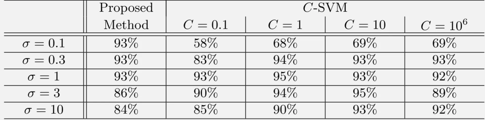
Experiments for Accuracy
Accuracy of binary classification:
It is not so worse than C-SVM.
December 1, ALSIP 2012
33
Binary Classification Using Fast Gaussian Filtering Algorithm 5
Table 1. Accuracy of classification of the Iris flower data set
(Classification between two species with 5-fold cross validation)
Proposed C-SVM Method C = 0.1 C = 1 C = 10 C = 106 σ = 0.1 93% 58% 68% 69% 69% σ = 0.3 93% 83% 94% 93% 93% σ = 1 93% 93% 95% 93% 92% σ = 3 86% 90% 94% 95% 89% σ = 10 84% 85% 90% 93% 92%
Table 2. Computational time to predict a class
(Every vector has two real numbers between 0 and 10, σ is 1)
# of training data 1,000 10,000 100,000 1,000,000
Proposed Prediction 2.43 ms 2.48 ms 2.55 ms 2.96 ms
method (Precomputation) (0.13 s) (1.48 s) (17.8 s) (203 s)
LIBSVM Prediction 0.02 ms 0.22 ms 2.29 ms 23.6 ms
(Training) (0.05 s) (4.47 s) (442 s) (1000+ s)
predicts a class by calculating all the distances between a target and training data. Precomputation of the proposed method takes nearly linear on the number of training data. Training of LIBSVM takes time that is nearly proportional to the square of the number of training data.
6 Conclusions
This paper showed that FGFA can be applied to sparse data using the d
-dimensional range tree algorithm. This is the same classification as a C-SVM
whose parameter C approaches 0, and it has as good accuracy as C-SVMs.
Ad-ditionally, we revealed that this can reduce time of prediction of C-SVMs when
the number of support vectors is larger than 10,000.
References
1. Kentaro Imajo. Fast Gaussian Filtering Algorithm Using Splines. In The 21st
International Conference on Pattern Recognition, 2012.
2. Koji Tsuda. Overview of Support Vector Machine. The Journal of the Institute of
Electronics, Information, and Communication Engineers, 83(6):460–466, 2000.
3. Christopher M. Bishop. Pattern Recognition and Machine Learning (Information
Science and Statistics). Springer-Verlag New York, Inc., 2006.
4. Chih-Chung Chang and Chih-Jen Lin. LIBSVM: A Library for Support Vector
Machines. ACM Transactions on Intelligent Systems and Technology, 2(3):27, 2011.
5. Jon Louis Bentley. Decomposable Searching Problems. Information Processing
Letters, 8(5):244–251, 1979.
6. R.A. Fisher. The Use of Multiple Measurements in Taxonomic Problems. Annals
of Human Genetics, 7(2):179–188, 1936.
Figure Accuracy for Iris Flower Data Set
/36
Experiments for Time
CPU time of training and prediction:
The proposed method is faster
when # of training data is over 150,000.
December 1, ALSIP 2012
34
Binary Classification Using Fast Gaussian Filtering Algorithm 5
Table 1. Accuracy of classification of the Iris flower data set
(Classification between two species with 5-fold cross validation)
Proposed C-SVM Method C = 0.1 C = 1 C = 10 C = 106 σ = 0.1 93% 58% 68% 69% 69% σ = 0.3 93% 83% 94% 93% 93% σ = 1 93% 93% 95% 93% 92% σ = 3 86% 90% 94% 95% 89% σ = 10 84% 85% 90% 93% 92%
Table 2. Computational time to predict a class
(Every vector has two real numbers between 0 and 10, σ is 1)
# of training data 1,000 10,000 100,000 1,000,000
Proposed Prediction 2.43 ms 2.48 ms 2.55 ms 2.96 ms
method (Precomputation) (0.13 s) (1.48 s) (17.8 s) (203 s)
LIBSVM Prediction 0.02 ms 0.22 ms 2.29 ms 23.6 ms
(Training) (0.05 s) (4.47 s) (442 s) (1000+ s)
predicts a class by calculating all the distances between a target and training data. Precomputation of the proposed method takes nearly linear on the number of training data. Training of LIBSVM takes time that is nearly proportional to the square of the number of training data.
6 Conclusions
This paper showed that FGFA can be applied to sparse data using the d
-dimensional range tree algorithm. This is the same classification as a C-SVM
whose parameter C approaches 0, and it has as good accuracy as C-SVMs.
Ad-ditionally, we revealed that this can reduce time of prediction of C-SVMs when
the number of support vectors is larger than 10,000.
References
1. Kentaro Imajo. Fast Gaussian Filtering Algorithm Using Splines. In The 21st
International Conference on Pattern Recognition, 2012.
2. Koji Tsuda. Overview of Support Vector Machine. The Journal of the Institute of
Electronics, Information, and Communication Engineers, 83(6):460–466, 2000.
3. Christopher M. Bishop. Pattern Recognition and Machine Learning (Information
Science and Statistics). Springer-Verlag New York, Inc., 2006.
4. Chih-Chung Chang and Chih-Jen Lin. LIBSVM: A Library for Support Vector
Machines. ACM Transactions on Intelligent Systems and Technology, 2(3):27, 2011.
5. Jon Louis Bentley. Decomposable Searching Problems. Information Processing
Letters, 8(5):244–251, 1979.
Figure Time of Training and Prediction for 2D Data
/36
1. Fast Gaussian Filtering Algorithm
2. Binary Classification Using
The Fast Gaussian Filtering Algorithm
3. Evaluations
4. Conclusions
December 1, ALSIP 2012
35
Conclusions
We proposed a new binary classifier. • It is not so worse than C-SVM, and
it can also speed up prediction of C-SVM. • Pre-computation is O(4dnlog2dn) time,
and prediction is O(4dlog2dn) time.
The proposed method consists of • Fast Gaussian filtering algorithm,