Can Oil Prices Predict Stock Market Returns?

(1)

Can Oil Prices Predict Stock Market Returns?

Kevin Daly (Corresponding Author)

School of Economics and Finance Locked Bag 1797, Penrith NSW 2751, Australia Tel: 61-2-4620-3546 E-mail: k.daly@uws.edu.au

Abdallah Fayyad

School of Economics and Finance Locked Bag 1797 Penrith NSW 2751, Australia

E-mail: A.Fayyad@uws.edu.au

Received: July 28, 2011 Accepted: August 16, 2011 Published: December 1, 2011 doi:10.5539/mas.v5n6p44 URL: http://dx.doi.org/10.5539/mas.v5n6p44

Abstract

This paper performs an empirical investigation into the relationship between oil price and stock markets returns for seven countries (Kuwait, Oman, UAE, Bahrain, Qatar, UK and USA) by applying the Vector Auto Regression (VAR) analysis. During this period oil prices have tripled creating a substantial cash surplus for the Gulf Cooperation Council (GCC) Countries while simultaneously creating increased deficit problems for the current accounts of the advanced economies of the UK & USA. The empirical investigation employs daily data from September 2005 to February 2010. Our empirical findings suggest the followings: (1) the predictive power of oil for stock returns increased after a rise in oil prices and during the Global Financial Crises (GFC) periods. (2) The impulsive response of a shock to oil increased during the GFC period. (3) Qatar and the UAE in GCC countries and the UK in advanced countries showed more responsiveness to oil shocks than the other markets in the study.

Keywords: Oil, Gulf Cooperation Council (GCC), UK and USA, Vector auto regression model, Variance decomposition, Impulse response function

1. Introduction

Oil prices have traditionally been more volatile than other commodity prices since World War II. The dynamics of demand and supply for oil in the global economy coupled with the activities of oil producers themselves ensures that an understanding of the volatile nature of oil prices is amongst the most topical pursuits of researcher’s. Recent changes in oil prices in the global economy have been rapid and unprecedented. This is partly due to the increased demand for oil by China and India.

The price of crude oil in US$ per barrel is tracked over a 38 year period in Figure 1 below. The Global Financial Crisis beginning in September 2008 was preceded by a year of less acute financial turmoil, which substantially reinforced the cyclical downturn in oil prices. At the beginning of 2008 the basket prices of oil was less US$100/b, middle of the year it was approximately US$140/b and by the year end the price was below US$40/b.

Early empirical studies by Gisser and Goodwin (1986) and Hickman et al. (1987)—confirmed an inverse relationship between oil prices and aggregate economic activity. Darby (1982), Burbidge and Harrison (1984), and Bruno and Sachs (1982, 1985) documented similar oil price-economy relationships in cross-country analysis. Hamilton (1983) made a definitive contribution by extending the analysis to show that all but one of the post-World-War-II recessions was preceded by rising oil prices, which other business cycle variables did not predict. Jones and Leiby (1996) find that the estimated oil price elasticity of GNP in the early studies ranged from -0.02 to -0.08, with the estimates consistently clustered around-0.05.

Several explanations have advanced as to why an inverse relationship exists between oil price movements and aggregate economic activity. Of these explanations, the classic supply-side model appears to be most favored by showing how rising oil prices slow GDP growth and stimulates inflation, in Rasche and Tatom (1977 and 1981), Barro (1984) and Brown and Yücel (1999). More recent studies by Gronwald (2008), Cologni and Manera (2008),

(2)

Kilian (2008), Lardic and Mignon (2006, 2008), and Lescaroux and Mignon (2008) have somewhat confirmed the earlier findings.

Apart from studies showing that oil price shocks have significant effects on economy’s performance, relatively few researchers have studied the relationship between oil prices and stock markets. In addition, most of this works has concentrated on developed oil importers with less focus on emerging markets or oil exporting countries. In this paper, we will focus on both oil- importing and oil- exporting countries.

The GCC established in 1981 includes six member countries of Bahrain, Oman, Kuwait, Qatar, Saudi Arabia and the United Arab Emirates (UAE). GCC countries share several common economic characteristics. In 2007, they produced in combination about 20% of all world crude oil, controlled 36% of world oil exports and acquired 47% of verified reserves. Oil exports largely determine earnings, government budget revenues, expenditures, and aggregate demand.

The GCC markets are important for several reasons.

GCC markets have attracted increasing attention in the last decade-in the wake of high oil prices since 2003 and recently in 2008, they have each achieved high economic growth rates.

GCC markets differ from those of developed and from those of major emerging countries in that they are predominately-segmented markets, largely isolated from the international markets and are overly sensitive to regional political events. Arouri, M. & Rault, C. (2010).

Jones and Kaul (1996) initial study focused on testing the reaction of advanced stock markets (Canada, UK, Japan, and US) to oil price shocks on the basis of the standard cash flow dividend valuation model. They found that for the US and Canada the reaction can be determined by the impact of the oil shocks on cash flows while the outcome for Japan and the UK were indecisive. Huang et al. (1996) applied unrestricted vector autoregressive (VAR) which confirmed a significant relationship between some US oil company stock returns and oil price changes. Conversely, they found no evidence of a relationship between oil prices and market indices such as the S&P500. In contract, Sadorsky (1999) applied an unrestricted VAR with GARCH effects to US monthly data and found a significant relationship between oil price changes and aggregate stock returns. Recently, El-Sharif et al. (2005) examined the links between oil price movements and stock returns in the UK oil and gas sector. They found a strong interrelationship between the two variables.

Abu Zarour, B. (2006), applied a VAR model to investigate the relation between oil prices and five stock markets in Gulf Countries during the period between May 2001 and May 2005. They found the response of these markets to shocks in oil prices increased and became faster during episodes of oil price increases.

Maghyereh, A. & AL-Kandari, A. (2007), found that oil price affects the stock price indices in GCC countries in a nonlinear fashion and they supported the statistical analysis of a nonlinear modeling relationship between oil and the economy, which is consistent with Mork et al. (1994), and Hamilton (2000).

Figure 2 shows how the stock markets in the GCC countries and oil prices are interrelated, it is apparent that both oil prices and stock market indices of the GCC countries have a common trend.

Miller & Ratti (2009) analyzed the long-run relationship between the world price of crude oil and international stock markets over the period from January 1971 to March 2008. They found a clear long-run relationship between the stock market prices of six OECD countries over the period 1971:1–1980.5 and 1988:2–1999.9, suggesting that stock market indices respond negatively to increases in the oil price over the long run. During 1980.6–1988.1, they find the relationships to be not statistically significantly different from either zero or from the relationships of the previous period. However, the expected negative long-run relationship appears to disintegrate after 1999.9. This finding supports a conjecture of change in the relationship between real oil price and real stock prices in the last decade compared to earlier years, which may suggest the presence of several stock market bubbles and/or oil price bubbles since the turn of the century.

Arouri and Rault, (2010), used the panel-data approach of Kónya (2006), based on seemingly unrelated regression (SUR) systems and Wald tests with Granger to study the sensitivity of stock markets to oil prices for GCC countries over the period from June 2005 to October 2008, and from January 1996 to December 2007. Their results indicate a strong statistically significant causal relationship, which was bi-directional for Saudi Arabia. However in the case of the other GCC countries, stock market price changes do not Granger cause oil price changes, whereas oil price shocks Granger cause stock price changes in a negative direction. This study suggests that changes in oil prices affect stock market returns in inversely for the majority of GCC countries.

(3)

2. Data and Empirical Results

The daily data employed in this study was sourced from the weighted equity market indices of seven stock markets namely Kuwait, Oman, United Arab Emirates (UAE), Bahrain, Qatar, United Kingdom (UK) and United States of America (USA and the Brent spot oil price. Out model employed daily data for the period 21/09/2005 — 12/02/2010, the stock market data was obtained from MSCI Barra while the daily data for crude oil price was sourced from the U.S. Department of Energy, Energy Information Administration (EIA).

All indices were based on US dollar and do not include dividends, the indices include small, medium and large capitalized firms. Returns for both stocks and oil are expressed in terms of percentage change by multiplying the first difference of the logarithm of stock market by 100.



P

_i



LOG

(

P

_it

/

P

_it_₁

)



100

Where



P

_i denotes the rate of change of

P

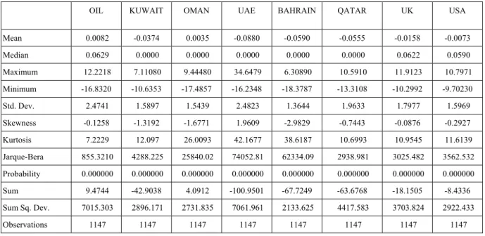
_it.

Table 1 presents the descriptive summary statistics of daily returns for the seven stock markets and oil for the period between 21/09/2005—12/02/2010. It is apparent from Table 1 results that the volatility (measured by standard deviation) for oil price (2.474178) is higher than all other markets since oil tripled during the study period from minimum value of $49.95 to $143.95.

The distributional properties of the return series appear to be non-normal, since all the markets have negative skewness except for UAE. The kurtosis in all markets, both developed and emerging, exceeds three, indicating a leptokurtic distribution.

The Jarque-Bera statistic and the associated

p



value

were used to test the null hypotheses that the daily distributions of returns are normally distributed. With all

p



value

equal to zero at the six decimal places, we reject the null hypothesis that returns for developed and emerging markets are well approximated by a normal distribution.

The following conditional expected return equation accommodates each market’s own returns and the returns of other markets lagged one period:

R t 



 AR t1 



t ………(1)

Where

R

_t is the

n



1

vector of daily return at time

t

for each market.

t



is the innovation for each market at time

t

with its corresponding

n



n

conditional variance - covariance matrix,



t . The market information available at time

t



1

is represented by the information

set

I

_t_₁. The

n



1

vector



represents long-term drift coefficients. The estimate of the elements of the matrix, A, can provide measures of the significance of the own and cross-mean spillovers. Figure 3 presents the markets daily returns, for the period between 21/09/2005 to 12/02/2010. We note that all stock markets in the study experienced significant volatility over the financial crisis especially during the month of September 2008 with the US, UK and perhaps Kuwait experiencing the higher ranges of that volatility. By comparison, the volatility in oil prices although apparent from the graph did not reach the heights recoded for stocks.

3. Methodology

3.1 Unit Root Test (URT)

We test for unit roots for each series (1st_{difference of raw data). We test the null hypothesis for the existence of a}

unit-root (non-stationary) against the alternative hypothesis of stationary variables using the Augmented Dickey–Fuller(ADF) statistic, Dickey, D.A., Fuller, W.A., 1981.We employ the Automatic selection of lags based on Schwarz (SIC), these results are available to readers on request .

3.2 VAR Methodology

The vector autoregressive (VAR) is commonly used for forecasting systems of interrelated time series and for analyzing the dynamic impact of random disturbances on the system of variables. The VAR approach bypasses the need for structural modeling by treating every variable as endogenous in the system as a function of the lagged values of all endogenous variables in the system. The term autoregressive is due to the appearance of the lagged values of the dependent variable on the right-hand side and the term vector is due to the fact that a vector of two (or more) variables is included in the system model, Hung, B. (2009).

The mathematical representation of a VAR system is

(4)

Or                                                                                                             pt t t t p k t k t k t k t pp p p p p p p p t t t t pp p p p p p p P t t t t e e e e Y Y Y Y A A A A A A A A A A A A A A A A Y Y Y Y A A A A A A A A A A A A A A A A Y Y Y Y ... ... ' ... ' ' ' ... ... ... ... ... ' ... ' ' ' ' ... ' ' ' ' ... ' ' ' ... ... ... ... ... ... ... ... ... ... ... ... 3 2 1 2 2 1 3 2 1 3 33 32 31 2 23 22 21 1 13 12 11 1 2 1 2 1 1 1 3 2 1 3 33 32 31 2 23 22 21 1 13 12 11 3 2 1

Where p is the number of variables be considered in the system, k is the number of lags be considered in the system,

   

Y

_t

,

Y

_t_₁

,...

 

Y

_t__k, are the

1



p

vector of variables, and the

 

A

,...

&

 

A



are the

p



p

matrices of coefficients to be estimated,

 

e

_t is a

1



p

vector of innovations that may be contemporaneously correlated but are uncorrelated with their own lagged values and uncorrelated with all of the right-hand side variables.

Since there are only lagged values of the endogenous variables appearing on the right-hand side of the equations, simultaneity is not an issue and OLS yields consistent estimates. Moreover, even though the innovations may be contemporaneously correlated, OLS is efficient and equivalent to Generalized Least Squares (GLS) since all equations have identical repressors.

For this study, suppose that stock market (SK) and Oil prices (O) are jointly determined by a VAR and let a constant be the only exogenous variable. Assuming that the VAR contains two lagged values of the endogenous variables, it may be written as





























































































    t t t t t t t t

e

C

O

SK

b

O

SK

a

O

SK

2 1 2 1 2 2 22 21 12 11 1 1 22 21 12 11 …………..(3) Or t k i k i i t i t i t

C

a

SK

b

O

e

SK

₁ 1 1 1 1 1 1



   





t k i k i i t i t i t

C

a

SK

b

O

e

O

₂ 1 2 1 2 1 2



   





Where

a

_ij

,

b

_ij

&

c

_ij are the parameters to be estimated, the

(

i

,

j

)

th

components reveals the response of the

ith

market return to a unit random shock in the

jth

market return after

k

periods also this represents

the impulse response of the

ith

market in

k

periods after a shock of one standard error in the

jth

market,

s

e

_i

'

are the stochastic error terms and are called innovations or shocks in the language of VAR.

As well, the variance decomposition of the forecast error gives us the percentage of unexpected variation in each market’s return that is produced by shocks from other returns in the system.

The VAR requires the determination of an appropriate lag structure in the system. In this study four lags have been chosen as oil is the main reference in this study. Lag structure is chosen based on the smallest value of Akaike (AIC) or Schwarz (BIC) of the VAR to determine the appropriate lags, Quantitative Micro Software, L. (2007).

3.3 VAR Estimation

In order to examine how changes in oil prices affect stock markets and the dynamic interrelationships between them we divided our estimation period into three sub-periods and estimated a VAR system for each period. The first period (normal period where oil prices appear constant: from 21 September 2005 to 06 October). Over the second period, (rise period where oil prices have increased above trend includes October 2006 to October 2008). The latter period includes the remarkable rise in oil prices, which tripled, from a minimum price of $49.95 per barrel to $143.95 per barrel. Finally, the third period (falling prices Global Financial Crises-GFC, F) includes the

(5)

timeframe from October 2008 to February 2010.

The estimation results of the VAR system for five GCC countries, UK, USA stock markets returns and oil returns for the first period (normal) (results are available from authors). The results indicate that there is no significant relationship between oil prices and the seven stock markets of the countries on a daily basis. The oil pries cannot predict or be predicted by any of the five GCC markets, UK or USA. However, a one-way directional relationship does appear from oil to the UK (-2) and Bahrain (-3) stock markets, (brackets represent lags). During the second period where oil price increase, our results from the estimated VAR indicate that, oil prices can predict UAE (-1), Kuwait (-3) and USA (-2) stock markets (lags are represented in brackets). Interestingly over this period of rising oil prices, the direction of oil price change can be predicted by most of the stock markets (Kuwait, Oman, Qatar, UK and USA), except UAE and Bahrain. In addition, the directional relationship between the GCC markets increased. One can find two-way directional relations between Omani and Kuwaiti stock markets and between Qatar and USA. Finally, the VAR estimation results for the third period (falling oil prices over the GFC); here oil prices can predict the direction of five stock market indices of Oman (-2), UAE (-2), Qatar (-1), UK (-1) and USA (-1) except Kuwait and Bahrain. Over this period of falling oil prices we observe that oil price changes can be predicted by Kuwait (-4), Bahrain (-2), Qatar (-3), UK (-2) and USA (-2) stock markets.

The results of the estimated VAR system for the second period (rising oil prices) reflect the fact that sharp increase in oil prices, did predict the direction of the US and two GCC countries stock markets, in comparison with the first period (constant oil price) that has normal oil prices and no prediction about stock market prices. It is noteworthy that over the third period of falling oil prices the predictive power of oil on stock markets increases. These results should not appear strange if we take into consideration that these countries essentially depends, in varying degrees, on oil, and that the GCC countries are the world’s biggest oil exporting country in addition to holding the largest oil reserves while other countries (USA and UK) are the biggest consumers of oil in the world.

3.4 Variance Decomposition

Variance decomposition measures the percentage of the forecast error of a market return that is explained by another market for instance oil market returns. It indicates the relative impact that one market has upon another market. The variance decomposition enables us to assess the economic significance of this impact as a percentage of the forecast error for a variable sum to one. The orthogonolization procedure of the VAR system decomposes the forecast error variance, the component that measures the fraction in stock return of a particular market explained by innovations in each of the seven indices, Abu Zarour, B. (2006).

Table 2 provides the variance decomposition of the 4 days ahead forecast error of each index for the so-called

normal oil price period. For the first period each row indicates the percentage of forecast error variance explained

by the market indicated in the first column, for instance at 4 period horizons for (KUWAIT) indicates that the 1.18% of forecast error variance in Kuwait is explained by the Oil market. The results indicate that most markets and oil returns are strongly exogenous in the sense that the percentage of the error variance accounted by the Kuwaiti market is approximately 93% at time horizon 4 while the percentage of the foreign explanatory power, as indicated by the all markets, is insignificant, reaching in the best cases 7% at time horizon 4.

Bahrain in the GCC markets is the least exogenous with 22% error variance explained by other markets; mainly the 11.6% explained by Kuwaiti markets, this means that the 11.6% of forecast error variance in Bahraini market is explained by the Kuwaiti market. Representing the advanced markets, the USA is the least exogenous with 33% error variance explained by other markets and mainly with 25.5% explained by UK market, this means that the 25.5% of forecast error variance in USA market is explained by the UK market. We can say that in both the GCC and advanced markets oil market plays a minor role in the forecast of error variance which matches with our results in of VAR estimation.

The variance decomposition for the second period (available from authors) shows that after a sharp rise in oil prices, one can find that in general all variables in the system have more endogenous power than the first period. The percentage of the foreign explanatory power is relatively strong; it exceed 44% for UAE, 27% for Bahrain, 45% for Qatar, 34% for UK and 42% for USA. The Kuwait market plays an important role during this period in the GCC markets while oil comes in the second, third and sometimes in fourth position. Since 12.5% of forecast error variance in Omani Market is explained by the Kuwaiti market, 19.3% in UAE, 17.6% in Bahrain and 17.5% in Qatar. For the advanced markets USA and UK plays a bidirectional role between each other.

Table 3 provides the variance decomposition for the third period (falling oil prices) covering the GFC. In the case of the GCC countries and after the fall in oil prices, Kuwait first, Oman second and oil third plays significant endogenous power for the GCC markets while oil has the first endogenous power for the Omani market (10% ) this

(6)

means that 10% of forecast error variance in Omani Market is explained by the Oil market. During this period, it is noticeable that oil has significant endogenous power for the advanced markets of USA and UK. Since 22.6% and 11.4% of forecast error variance in USA and UK Markets is explained by the oil market. In general the results achieved in this study cannot help us to verify which the dominant market is in the system that manipulates all the others and link their interdependence.

3.5 Impulse Response

The estimated impulse response of the VAR system enables us to examine how each of the seven variables responds to innovations from other variables in the system. These IM responses for all markets to one standard deviation shock in each of the GCC markets for the three periods are available on request form the authors. These results present the accumulated responses of all markets returns to one standard deviation shock in oil return for each period. In general, the responses are small and decline very slowly indicating that markets are not efficient in responding to a shock generated from oil returns. However, it is noticeable that a shock in oil price has a major and persistence impact on UAE, Qatar and UK markets more than on other GCC and USA markets. It requires the Qatar market two days to start responding to a shock to oil returns. In addition, Oman, Qatar and UK markets respond positively while other markets respond negatively to shock in oil returns.

For the second period, which witnesses the sharp rise in oil prices, we have a different picture for the relationship between GCC, UK, USA stock markets and oil returns. The Qatar market stands out to be the most influenced followed by UAE market then the Omani market. All markets react from the first day. It seems that these markets react quickly, appear relatively efficient since their reactions taper off, and start declining after day 11 to a shock originated in oil returns. However, Kuwait and USA markets show a small and slow process in responding to oil shock while Oman and Qatar markets show big and quick response.

The accumulated response of all markets returns to one standard deviation shock in oil return for the third period (fall) indicates that despite falling oil prices there is a positive response for all markets we should note that during this period the GFC was most vigorous. For the GCC markets, it is noticeable that UAE has a major positive and persistence response followed by Oman, Qatar, Kuwait and Bahrain. For the advanced markets, UK market has the major response followed by USA market. Regardless of the different magnitude of impulse response values, some of the above-mentioned Tables and Figures require comment.

For the first period (constant oil price), the response of the GCC stock markets to a shock in oil returns seems to be small and tapers off slowly from day 4 for all markets except for Qatar and the UK, which indicates a positive and persistent response. On the other hand, the US market shows a lesser degree of response compared to all the other markets.

For the second period (rising oil prices), after oil prices dramatically increase, the interaction between oil returns and all stock markets increased especially for Qatar, UAE, Oman, Bahrain and Kuwait. The latter all exhibit large and quick responses to oil shocks within a 4-day horizon. Over this period, the UK displays a faster and bigger response than USA market.

The Qatar market exerts the greatest response when oil prices rise; this is not surprising since approximately 42% of its GDP is derived from oil, second after Saudi Arabia with 44%.

For the third period (GFC period), the relationships between oil returns and all the stock markets increased especially for the UAE, Oman, Qatar, Kuwait and Bahrain. They each exhibit large and quick responses to oil shocks within a 7-day horizon. The UAE results are not surprising because the UAE market is more liberalized comparing to other GCC markets since half of the listed companies on the UAE exchange allow non-GCC stock ownership. The UK shows a faster and larger response within a 6-day horizon compared to the USA market. These results reflect the significant impact of the increase in oil prices on GCC stock markets. This is quite normal since GCC countries produce about 21% of the world’s daily oil production and they possess about 43% of the world’s oil reserve.

4. Conclusion

This paper uses Vector Auto-Regression (VAR), DCV and Impulse Response techniques to examine the effects of changes in oil prices on the GCC countries, the UK, and the US stock markets. These techniques allow us to examine the dynamic structures between the five member countries of the oil rich GCC and the advanced countries of the UK, USA in terms of the inter-relationships between oil and stock market returns. To achieve the primary objective of the study which focuses on the inter relationships between oil and stock markets, the period of estimation was divided into three sub-period referred to as constant, rising and falling oil price episodes.

(7)

The empirical results suggest the following: (1) Oil return cannot predict or be predicted by any GCC, UK, and USA stock market for the first period. However, after the oil prices rose sharply during the second period, oil can predict Kuwait, UAE and USA stock markets but not Qatar, Bahrain, Oman and UK. During the third period of GFC, all markets can be predicted by oil except Kuwait and Bahrain. (2) The variance decomposition indicates that all variables in the system are generally exogenous, while in the second period, the results look more endogenous since error forecast reaches up to 45% of the UAE can be explained by other stock markets and oil, while for the advanced markets it reaches up to 42% for USA. (3) The impulse responses functions indicate that for the first period the responses of GCC markets to shocks in oil returns were of a small order in general. During the second and third periods the GCC, UK and US markets’ responses are significantly greater than the period of constant oil price. (4) The response of stock returns for all markets to shocks generated by oil was large and characterized by prolonged memory during the third period (GFC).

From an economic point, the results suggest that there is a significant inter-relationship between the GCC markets. Oil prices do affect GCC markets and advanced market of UK and USA but to varying degrees. A high priority for policy makers in GCC countries is to diversify their economies by increasing the contributions of the non-oil sector to GDP. This is particularly important given that oil shocks impact sharply not only on GCC countries GDP but also the stock market returns.

References

Abu Zarour, B. (2006). Wild oil prices, but brave stock markets! The case of GCC stock markets. Operational

Research. An International Journal,6, 145-162.

Arouri, M., & Rault, C. (2010). Oil Prices and Stock Markets: What Drives what in the Gulf Corporation Council Countries? CESifo Working Paper, No.960.

Balaz, P., & Londarev, A. (2006). Oil and its position in the process of globalization of the world economy.

Politicka Ekonomie, 54(4), 508-528.

Bley, J., & Chen, K. (2006). Gulf Cooperation Council (GCC) stock markets: The dawn of a new era. Global

Finance Journal,17, 75-91. http://dx.doi.org/10.1016/j.gfj.2006.06.009

Brown, S. P. A., & Yücel, M. K. (2002). Energy Prices and Aggregate Economic Activity: An Interpretative Survey. The Quarterly Review of Economics and Finance, 42, 193-208. http://dx.doi.org/10.1016/S1062-9769(02)00138-2

Cologni, A., & Manera, M. (2008). Oil prices, inflation and interest rates in a structural co-integrated VAR model for the G-7 countries. Energy Economics.30, 856-88. http://dx.doi.org/10.1016/j.eneco.2006.11.001

Cunado, J., & Perez de Garcia, F. (2005). Oil prices, economic activity and inflation: evidence for some Asian countries. The Quarterly Review of Economics and Finance, 45, 1, 65-83. http://dx.doi.org/10.1016/j.qref.2004.02.003

Dickey, D. A., & Fuller, W. A. (1981). Likelihood ratio statistics for autoregressive time series with a unit root.

Econometrica. 49, 1057–1072. http://dx.doi.org/10.2307/1912517

El-Sharif, I., Brown, D., Burton, B., Nixon, B., & Russell, A. (2005). Evidence on the nature and extent of the relationship between oil prices and equity values in the UK. Energy Economics, 27, 819-830. http://dx.doi.org/10.1016/j.eneco.2005.09.002

Gronwald, M. (2008). Large oil shocks and the US economy: Infrequent incidents with large effects. Energy

Journal, 29, 151-71. http://dx.doi.org/10.5547/ISSN0195-6574-EJ-Vol29-No1-7

Hamilton, J. D. (2000). What is an oil shock. Working paper, No. W7755, MBER.

Hammoudeh, S. & Aleisa, E. (2004). Dynamic relationships among GCC stock markets and NYMEX oil futures.

Contemporary Economic Policy, 22(2), 250-69. http://dx.doi.org/10.1093/cep/byh018

Huang, R. D., Masulis, R. W., & Stoll, H. R. (1996). Energy shocks and financial markets. Journal of Futures

Markets, 16, 1-27. http://dx.doi.org/10.1002/(SICI)1096-9934(199602)16:1<1::AID-FUT1>3.0.CO;2-Q

Hung, B. (2009) Vector Auto-regression (VAR) model. retrieved on April 25, 2010. [Online] Available: http://www.hkbu.edu.hk/~billhung/econ3670/lecture/3670note10.doc

Jones, C. M., & Kaul, G. (1996). Oil and the Stock Markets. Journal of Finance, 51(2), 463-491. http://dx.doi.org/10.2307/2329368

(8)

Economy. Review of Economics and Statistics,90, 216-40. http://dx.doi.org/10.1162/rest.90.2.216

Kónya, L. (2006). Exports and growth: Granger causality analysis on OECD countries with a panel data approach.

Economic Modelling,23: 978-982. http://dx.doi.org/10.1016/j.econmod.2006.04.008

Lardic, S., & Mignon, V. (2008). “Oil prices and economic activity: An asymmetric co-integration approach” .

Energy Economics, 30(3), 847-855. http://dx.doi.org/10.1016/j.eneco.2006.10.010

Lardic, S. & Mignon, V. (2006). The impact of oil prices on GDP in European countries: An empirical investigation based on asymmetric co-integration. Energy Policy, 34(18), 3910-3915. http://dx.doi.org/10.1016/j.enpol.2005.09.019

Lescaroux, F., & Mignon, V. (2008). On the influence of oil prices on economic activity and other macroeconomic

and financial variables. OPEC Energy Review, 32(4), 343-380.

http://dx.doi.org/10.1111/j.1753-0237.2009.00157.x

Maghyereh, A., & AL-Kandari, A. (2007). Oil prices and stock markets in GCC countries: new evidence from nonlinear co-integration analysis. Managerial Finance, 33, 449-460. http://dx.doi.org/10.1108/03074350710753735

Miller, I., & Ratti, R. (2009). Crude oil and stock markets: Stability, instability, and bubbles. Energy Economics,31, 559-568. http://dx.doi.org/10.1016/j.eneco.2009.01.009

Mork, K. A., Olsen, O., & Mysen, H.T. (1994). Macroeconomic responses to oil price increases and decreases in seven OECD countries. Energy Journal. 15, 19-35.

Papapetrou, E. (2001).Oil Price Shocks, Stock Market, Economic Activity and Employment in Greece. Energy

Economics, 23, 511-32. http://dx.doi.org/10.1016/S0140-9883(01)00078-0

Quantitative Micro Software, L. (2007). EViews 6 User’s Guide II (6 ed), Chapter 34.

Sadorsky, P. (1999).Oil Price Shocks and Stock Market Activity. Energy Economics, 2, 449-469. http://dx.doi.org/10.1016/S0140-9883(99)00020-1

Notes

Note 1: Real Oil prices have been rescaled to be comparable with the average of the GCC real stock market indices Table 1. Summary statistics of daily return for seven stock markets and oil

OIL KUWAIT OMAN UAE BAHRAIN QATAR UK USA

Mean 0.0082 -0.0374 0.0035 -0.0880 -0.0590 -0.0555 -0.0158 -0.0073 Median 0.0629 0.0000 0.0000 0.0000 0.0000 0.0000 0.0622 0.0590 Maximum 12.2218 7.11080 9.44480 34.6479 6.30890 10.5910 11.9123 10.7971 Minimum -16.8320 -10.6353 -17.4857 -16.2348 -18.3787 -13.3108 -10.2992 -9.70230 Std. Dev. 2.4741 1.5897 1.5439 2.4823 1.3644 1.9633 1.7977 1.5969 Skewness -0.1258 -1.3192 -1.6771 1.9609 -2.9829 -0.7443 -0.0876 -0.2927 Kurtosis 7.2229 12.097 26.0093 42.1677 38.6187 10.6993 10.9545 11.6139 Jarque-Bera 855.3210 4288.225 25840.02 74052.81 62334.09 2938.981 3025.482 3562.532 Probability 0.000000 0.000000 0.000000 0.000000 0.000000 0.000000 0.000000 0.000000 Sum 9.4744 -42.9038 4.0912 -100.9501 -67.7249 -63.6768 -18.1505 -8.4336 Sum Sq. Dev. 7015.303 2896.171 2731.835 7061.961 2133.625 4417.583 3703.824 2922.433 Observations 1147 1147 1147 1147 1147 1147 1147 1147

(9)

Table 2. Countries Variance Decomposition

Period S.E. OIL UAE BAHRAIN QATAR UK USA

1 1.1403 0.1188 0.0000 0.0000 0.0000 0.0000 0.0000 2 1.1577 1.1672 0.0036 0.0511 1.1617 0.2070 0.1702 3 1.1645 1.1711 0.2444 0.2085 1.2327 0.2455 0.3343 4 1.1864 1.1822 0.8080 0.2033 1.8525 0.2797 1.1262

1 1.1363 0.7312 0.311994 83.715 0.0000 0.0000 0.0000 2 1.1541 0.7220 0.837091 82.558 0.0219 0.01052 0.0257 3 1.1773 1.1743 1.391644 79.346 1.5882 0.1185 0.9534 4 1.1926 1.1491 1.742805 77.979 1.5549 0.1157 1.4995

1 0.6899 0.3800 0.2338 0.3019 0.0583 25.7980 73.0030 2 0.7099 0.5051 2.1730 1.0997 0.0594 25.5780 69.0020 3 0.7316 0.5162 2.3359 1.0420 0.5566 24.1270 68.0800 4 0.7354 0.5316 2.3115 1.1069 0.5514 24.4920 67.3900

Table 3. Variance Decomposition for the Forecast Error of Daily Market Returns for GCC Markets, UK, USA and OIL Markets during the Third Period (fall)

Variance Decomposition of OMAN:

Period S.E. OIL KUWAIT OMAN UAE BAHRAIN QATAR UK USA

1 1.7526 0.4687 7.4401 92.0911 0.0000 0.0000 0.000000 0.0000 0.0000 4 2.0487 10.0238 8.7225 69.8025 0.6774 0.1868 0.4455 7.1874 2.9538

Variance Decomposition of UK:

1 2.1751 26.9682 1.5487 0.0398 0.5056 1.0933 0.2467 69.5973 0.0000 4 2.4036 22.6729 1.9513 1.0788 1.4991 1.2620 0.2405 58.6570 12.6381

Variance Decomposition of USA:

1 2.1051 12.6936 0.0050 0.2230 0.3721 0.5089 0.0073 33.2443 52.9454 4 2.2396 11.4800 1.8368 1.8158 2.2481 1.7840 1.4775 31.1466 48.2108

(10)

Figure 1. Crude Oil Prices 1970 to 2009(Source OPEC Bulletin Dec 2010) 200 400 600 800 1000 1200 1400 1600 100 200 300 400 500 600 700 800 900 OIL KUWAIT OMAN UAE BAHRAIN QATAR

(11)

-20 -10 0 10 20 2006 2008 2009 OIL -12 -8 -4 0 4 8 2006 2008 2009 K U W A IT -20 -10 0 10 2006 2008 2009 O M A N -20 -10 0 10 20 30 40 2006 2008 2009 U A E -20 -10 0 10 2006 2008 2009 B A H R A IN -20 -10 0 10 20 2006 2008 2009 Q A T A R -15 -10 -5 0 5 10 15 2006 2008 2009 U K -10 -5 0 5 10 15 2006 2008 2009 U S A