Knowledge Gradient Methods for Bayesian Optimization

(1)

KNOWLEDGE GRADIENT METHODS

FOR BAYESIAN OPTIMIZATION

A Dissertation

Presented to the Faculty of the Graduate School of Cornell University

in Partial Fulfillment of the Requirements for the Degree of Doctor of Philosophy

by Jian Wu August 2017

(2)

c

(3)

KNOWLEDGE GRADIENT METHODS FOR BAYESIAN OPTIMIZATION

Jian Wu, Ph.D. Cornell University 2017

Bayesian optimization, a framework for global optimization of expensive-to-evaluate functions, has shown success in machine learning and experimental design because it is able to find global optima with a remarkably small number of poten-tially noisy objective function evaluations. In this dissertation, we study in detail how the concept of the knowledge gradient (KG) can be adopted to design novel Bayesian optimization algorithms.

First, we propose a novel parallel Bayesian optimization algorithm by gener-alizing the concept of KG from the fully sequential setting to the parallel setting (qKG). By construction, this method provides a one-step Bayes-optimal batch of points to sample. We provide an eﬃcient strategy for computing this Bayes-optimal batch of points, and we demonstrate that the parallel knowledge gradient method finds global optima significantly faster than previous batch Bayesian optimization algorithms on both synthetic test functions and when tuning hyperparameters of practical machine learning algorithms, especially when function evaluations are noisy.

Second, we present a novel discretization-free strategy to calculate the set of points to be evaluated under the knowledge gradient method when used over an continuous domain. KG methods are widely studied for discrete ranking and se-lection problems, and provide a one-step Bayes-optimal point to sample, but all the previous eﬀorts generalizing KG to continuous domains rely on a discretized

(4)

finite approximation due to the computational challenges in calculating KG. How-ever, the discretization introduces error, and scales poorly as the dimension of the domain grows. In this chapter, we develop a fast discretization-free knowledge gradient method for Bayesian optimization, which is useful for all settings where KG is used over an continuous domain that overcomes these challenges.

Third, we explore the “what, when, and why” of Bayesian optimization with derivative information. We also develop a Bayesian optimization algorithm that eﬀectively leverages gradients. This algorithm accommodates incomplete and noisy gradient observations, can be used in both the sequential and batch settings, and can optionally reduce the computational overhead of inference by selecting the single most valuable directional derivative to retain. For this purpose, we develop a novel acquisition function, called the derivative-enabled knowledge-gradient (dKG). This generalizes the previously proposed batch knowledge gradient method to the derivative setting. We also provide a theoretical analysis of the algorithm: it is one-step Bayes-optimal by construction when derivatives are available, and we show (1) that it provides one-step value greater than in the derivative-free setting; and (2) that its estimator of the global optimum is asymptotically consistent.

Fourth, we show some preliminary results on how KG can be adopted to set-tings where we have some low-fidelity but cheap approximations. To this end, we develop a novel Bayesian optimization algorithm, continuous-fidelity knowledge gradient (cfKG), which can adaptively choose both the fidelity and the desired point to sample by better balancing the trade-oﬀ between the information gain vs. the cost when we have some continuous parameters controlling the fidelity of the information source we can query. Some preliminary numerical results are shown.

(5)

BIOGRAPHICAL SKETCH

Jian Wu was born in Hefei, Anhui province in China, a beautiful city in the middle of China. Before his college, he spent most of his time at his hometown. From age sixteen, he began his wonderful college life at Tsinghua, where he received a B.Eng in Automation. During his stay in Tsinghua, he obtained a foundation in math and computer science, which provides many building blocks for the work in this dissertation. Since joining Cornell ORIE, he has been interested in many practical problems arising in modern society including materials design [86], queueing theory [7, 8] and Bayesian optimization [84, 87].

(6)

To my wife, Linran.

(7)

ACKNOWLEDGEMENTS

I am grateful to many those who have contributed towards completing this disser-tation.

First and foremost, I would like to thank my advisors, Professor Peter I. Frazier and Jim Dai, for their constant help throughout my stay at Cornell. Their ways of defining and thinking about problems inspire me a lot. I am also grateful for their encouragements when sometimes I decided to pursue my own ideas. Pro-fessor Frazier’s willingness to apply Operations Research to solve problems from very diversified fields teaches me how useful OR can be. I also thank Professor Frazier, for his financial support for attending academic conferences, to providing computational resources.

I am also grateful to my family. Especially, I would like to thank my wife, Linran, for her love and trust. This work will not be possible without her. I dedicate this thesis to her.

Finally, I would like to thank my school of Operations Research & Information Engineering at Cornell, for the super productive and collaborative environment.

(8)

LIST OF FIGURES

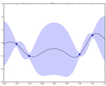
1.1 Illustration of Gaussian process regression with noisy evaluations on a 1-d function. The dots show previously evaluated points, (x(i), f(x(i))). The solid line shows the posterior mean,µ(n)(x)as a function ofx, which is an estimate f(x), and the shadow area show a Bayesian confidence interval for eachf(x), calculated as µ(n)(x)±1.96σ(n)(x). . . 7

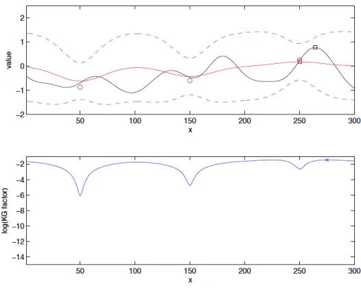
1.2 The source is at https://people.orie.cornell.edu/pfrazier/presentations. html. One should note that we are solving the maximization problem in this figure (instead of the minimization problem in (1.2.1)).The Upper panel shows the posterior distribution in a randomly sampled problem with independent normal homoscedastic noise and a one-dimensional input space, where the black solid line is the true function, the circles are previously measured points, the red solid line is the posterior mean

µ(n)₍_x₎_{, and the red dashed lines are at} _µ(n)₍_x₎_±₁_.₉₆_σ(n)₍_x₎_{. Lower} panel shows the natural logarithm of the knowledge gradient factorKG(x)

computed from this posterior distribution. An “x” is marked at the point with the largest KG factor, which is where the KG algorithm would evaluate next. . . 13

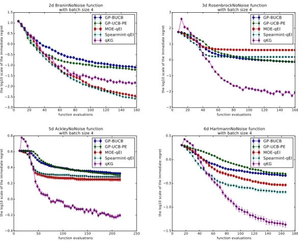
2.1 Performances on noise-free synthetic functions with q = 4. We report the mean and the standard deviation of the log10 scale of the immediate regret vs. the number of function evaluations. . . 30

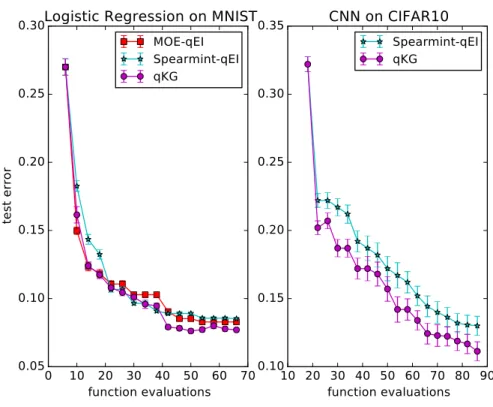
2.2 Performances on tuning machine learning algorithms withq = 4 . . . . 31

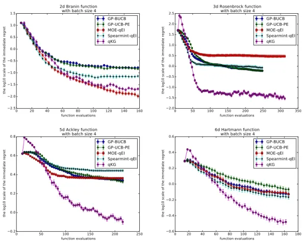
2.3 Performances on noisy synthetic functions with q = 4. We report the mean and the standard deviation of the log10 scale of the immediate regret vs. the number of function evaluations. . . 33

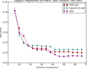
2.4 Tuning logistic regression on smaller test sets withq = 4 . . . 34

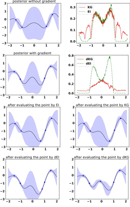
4.1 The topmost plots show (1) the posterior surfaces of a function sampled from a one dimensional GP with and without incorporating observations of the gradients. Note that the posterior variance is smaller if the gra-dients are incorporated; (2) the utility of sampling each point under the value of information criteria of KG and EI in both settings. If no derivatives are observed, both KG and EI will query a point with high potential gain (i.e. a small expected function value). On the other hand, when gradients are observed,d-KGmakes a considerably better sampling decision, whereasd-EI samples essentially the same location asEI. The plots in the bottom row depict the posterior surfaceafter the respective sample. Interestingly, KG benefits more from observing the gradients than EI (the last two plots): d-KG samples a point whose observation yields an accurate knowledge of the location of the optimum, whiled-EI still has considerable uncertainty around the optimum. . . 52

(11)

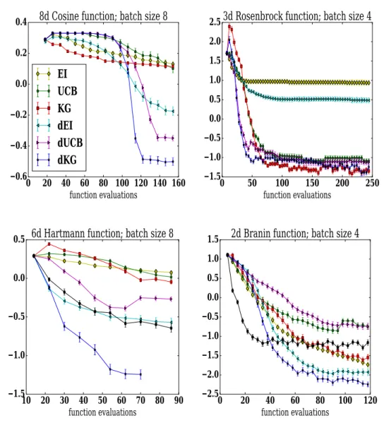
4.2 The average performance of 100 replications (the log10 of the immediate regret vs. the number of function evaluations). d-KG performs signifi-cantly better than its competitors for all benchmarks. In Branin and Hartmann, we also plot black lines, which is the performance of BFGS. . 58

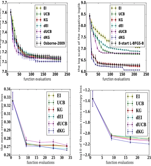
4.3 Results for the weighted KNN benchmark, the spectral mixture kernel benchmark, logistic regression and deep neural network (from left to right), all with batch size8 and averaged over 20replications. . . 61

5.1 The comparisons between KG and continuous-fidelity KG on three syn-thetic functions: Branin, 3-d Hartmann, and Rosenbrock. The fidelity space is one dimensional for Branin and Hartmann3 and two dimensional for Rosenbrock. . . 66

A.1 The performances of q-KG with diﬀerent batch sizes. We report the mean and the standard deviation of the log10 scale of the immediate regret vs. the number of iterations. Iteration 0 is the initial designs. For each iteration later, we evaluateq points recommended by theq-KG algorithm. . . 72

B.1 The average performance of 100 replications (the log10 of the immediate regret vs. the number of function evaluations) for the Levy and Ackley functions. For the Ackley function, we assume that a noisy observation of the full gradient is available. On the Levy function only 4th partial derivative can be observed (with noise). d-KG performs significantly better than its competitors for all benchmarks except the Levy function. 81

(12)

CHAPTER 1 INTRODUCTION

This thesis considers global optimization of expensive functions, in which (1) our objective function is expensive to evaluate (in terms of resources, money, time, etc), such that the number of function evaluations we can perform is extremely limited; (2) evaluating the objective function provides the noisy value of the objective, and

possibly some partial derivatives obscured by noise; (3) the objective function lacks structure beyond continuity such as convexity or submodularity; (4) we seek a global, rather than a local, optimum. Such problems typically arise when the objective function is evaluated by running a complex computer code (e.g. materials design [15], hyperparameter tuning [66], or algorithm configuration [26]), but also arises when the objective function can only be evaluated by performing a labor-intensive experiment, or running A-B tests in the real world.

Bayesian optimization (BO) methods are one class of methods attempting to solve such problems, and contain two components: (1) a statistical model: they use machine learning to build a statistical model for the unknown objective function, and the model provides not only point predictions but uncertainty quantifications; (2) an acquisition function: they use a carefully designed acquisition function to

suggest which point(s) in the function’s domain would be the most valuable to evaluate next. The acquisition function should balance the trade-oﬀ between ex-ploration and exploitation.

The most common statistical model in BO is to put a Gaussian process [61] prior distribution on the functionf, updating this prior distribution with each new observation of f. Some other models such as random forest [26] or deep neural

(13)

ing the next point or points to evaluate include probability of improvement (PI) [74], expected improvement (EI) [30], upper confidence bound (UCB) [71], entropy search/predictive entropy search (ES/PES) [22, 23], and knowledge gradient (KG) [62]. By carefully measuring the benefit of sampling at a point, BO often finds “near optimal” function values with fewer evaluations in comparison with other global optimization algorithms [66].

To the best of our knowledge, BO was pioneered in [37] followed by several seminal papers in the 1970s and 1980s pursued in [53] and [51]. In the late 1990s, Jones, Schonlau, and Welch introduced the famous Eﬃcient Global Optimization (EGO) method [30], building on the previous work by Mockus [51]. It used the Gaussian process (GP) as its statistical model and employed the EI acquisition function. This method became very popular and well-known in engineering, where it has been adopted for many time-consuming engineering design applications. In the 2000s, many follow-up works in statistics and engineering [24, 46] continued the successful story of BO. Since 2010s, interest in BO rose in the machine learning community, with publications including [26,66], after it was discovered BO was an excellent tool for tuning hyperparameters of computationally expensive machine learning models. If one is interested in knowing more about Bayesian optimization, [4] serves as a basic tutorial article and [64] gives a comprehensive review of some ongoing developments in BO.

In this chapter, we first enumerate a few problems arising from engineering design, materials discovery, medical science and machine learning that are suit-able for Bayesian optimization in Section 1.1. We then present the mathematical formulation of problems considered by Bayesian optimization in Section 1.2, and introduce the most common statistical model used by Bayesian optimization, i.e.

(14)

the Gaussian Process (GP), in Section 1.2.1, and common acquisition functions (the criteria for suggesting the point(s) to evaluate next) in Section 1.2.2. Finally, we provide an overview for the rest of the thesis in Section 1.3.

1.1

Examples Problems

The problems that can be solved by Bayesian optimization are incredibly common in practice. We enumerate a few examples from a long list, arising from a diversified set of fields. Some of these examples (such as machine learning hyperparameter tuning) will be considered more fully in the later chapters, and others are included to underscore the broad applicability of Bayesian optimization.

• Materials design and discovery: We would like to choose the chemical structure, composition, or processing conditions of a material to meet some design criteria. The evaluation usually requires physical experiments which are both time-consuming and expensive. Therefore, we choose the design adaptively by BO and test how good it is. See [15].

• Drug discovery: We would like to choose a molecule among a large pool to find the one that best treats a given disease. Synthesizing and testing a com-pound may require days and a significant investment of lab materials, which strictly limits the number of tests. Therefore, we test the molecules adap-tively by BO, and then collect information about its eﬀectiveness. See [55]. • Algorithm configuration: We would like to choose the algorithm

param-eters of some start-of-art solvers for hard computational problems. Each configuration evaluation is time-consuming and takes a lot of computational

(15)

the information about their empirical performance on standard benchmarks. See [26].

• Adaptive MCMC: We would like to choose the parameters in the Hybrid Monte Carlo (HMC) algorithm, such as step size, to ensure mixing of the Markov chain. Each parameter evaluation requires running HMC on the whole training data and is time-consuming. Therefore, we choose the param-eters adaptively by BO. See [47].

• Reinforcement learning: We would like to choose a parametric policy in a challenging Reinforcement Learning (RL) application. BO is attractive for this problem because it exploits Bayesian prior information about the expected return and exploits this knowledge to select new policies to execute. Eﬀectively, the BO framework for policy search addresses the exploration-exploitation tradeoﬀ. See [44].

• Machine learning hyperparameter tuning: For some machine learning algorithms, e.g., deep neural networks, using high-quality hyperparameters instead of low-quality ones is the diﬀerence between state-of-the-art predic-tive performance and being essentially useless. Typical approaches to tun-ing hyperparameters include hand tuntun-ing by experts and brute-force search. However, as the number of parameters grow, these approaches quickly be-come infeasible. To overbe-come this challenge, BO can be used to automate hyperparameter tunning. See [66].

(16)

1.2

Bayesian Optimization

In conventional Bayesian optimization (BO) [30], we wish to optimize a derivative-free expensive-to-evaluate function f with feasible domainA⊆Rd,

min

x∈Af(x), (1.2.1)

with as few function evaluations as possible. In this thesis, we assume that member-ship in the domainAis easy to evaluate and we can evaluatef only at points inA. We assume that evaluations off are either noise-free, or have additive independent normally distributed noise.

In many real problems, we do not know any structure information of the objec-tive function such as convexity or submodularity, and can only hope to obtain an estimate of the function value through running simulations or conducting physical experiments. Derivative information about the objective functions is not available in most of cases (that is why BO often belongs to the class of derivative-free opti-mization methods). Moreover, estimatingf(x)is usually an expensive process, for example, training a complex machine learning model such as denseNet [25] on a huge dataset such as ImageNet takes several days; conducting physical experiments requires labor investment of researchers and consumes resources.

Bayesian optimization is particularly suitable for these problems, when the ob-jective function does not have an explicit form, derivative information is not readily available, and function evaluation is expensive. BO consists of two components: a statistical model and an acquisition function. We will go over one by one: first, Bayesian optimization can incorporate the expertise belief about the problem in the form of a Bayesian prior; second, the sampling approach is designed to balance

(17)

evaluations required to find the optimum. We will review both aspects in details in Section 1.2.1 and Section1.2.2.

1.2.1

Gaussian Processes

Since the objective function is assumed unknown, in Bayesian optimization, we first build a predictive model on the objective function using Bayesian statistics. Among the wide variety of Bayesian statistical methods, Gaussian Process (GP) regression is a popular choice in Bayesian optimization. A Gaussian Process is a probability distribution over functions. Under the Gaussian Process, the marginal probability distribution of the value of the function at any single point is a normal distribution. The joint distribution of the values of the function at any collection of points is a multivariate normal distribution.

In Gaussian process regression, we use a Gaussian Process as our prior proba-bility distribution over the unknown objective function. We put a Gaussian pro-cess prior over the function f : A → R, which is specified by its mean function µ(x) : A → R and kernel function K(x1,x2) : A×A → R. We assume either

exact or independent normally distributed measurement errors, i.e. the evaluation

y(xi)at point xi satisfies

y(xi)|f(xi)∼ N(f(xi), σ2(xi)),

whereσ2 :A→R+is a known function describing the variance of the measurement errors. If σ2 _{is not known, we can also estimate it by either} _{maximum likelihood}

estimation (MLE) or in the fully Bayesian way.

(18)

Figure 1.1: Illustration of Gaussian process regression with noisy evaluations on a 1-d function. The dots show previously evaluated points,(x(i), f(x(i))). The solid line shows the posterior mean,µ(n)(x)as a function ofx, which is an estimatef(x), and the shadow area show a Bayesian confidence interval for eachf(x), calculated asµ(n)(x)±1.96σ(n)(x).

obtained corresponding measurements y(1:n)_{, we can then combine these observed}

function values with our prior to obtain a posterior distribution onf. This poste-rior distribution is still a Gaussian process with the mean function µ(n) _{and the}

kernel functionK(n) as follows

µ(n)(x) = µ(x) +K(x,x(1:n)) ( K(x(1:n),x(1:n)) +diag{σ2(x(1)),· · · , σ2(x(n))})−1(y(1:n)−µ(x(1:n))), K(n)(x1,x2) =K(x1,x2) −K(x1,x(1:n)) ( K(x(1:n),x(1:n)) +diag{σ2(x(1)),· · · , σ2(x(n))})−1K(x(1:n),x2). (1.2.2)

Figure 1.1 shows the output from Gaussian process regression on a one-dimensional function. [15] oﬀers a comprehensive review of Gaussian process regres-sion, including the choice of the mean function and the kernel function, inference with noisy observations, and hyperparameters estimation.

(19)

1.2.2

Acquisition Functions

The second crucial piece of Bayesian optimization is making good decisions about where to direct future sampling. Bayesian optimization methods address this by using a measure of the benefit that would be gained by sampling at a point, com-monly known as an “acquisition function”. Much of the literature in BO focuses on designing good acquisition functions that reach optima with as few evaluations as possible. Maximizing this acquisition function usually provides a single point to evaluate next, with common acquisition functions for sequential Bayesian op-timization including probability of improvement (PI) [37], expected improvement (EI) [30, 52], upper confidence bound (UCB) [71], entropy search/predictive

en-tropy search (ES/PES) [22, 23], and knowledge gradient (KG) [13, 62]. We will introduce some of these acquisition functions most relevant to this thesis in details.

Probability of Improvement

Considering the setting of noise-free function evaluations, the early work of [37] suggested maximizing the probability of improvement over the best sampled value observed so far, written as

PI(x) = P(f(x)≤f_n∗−ϵ), (1.2.3) where f_n∗ = minm≤nf(x(m)), is the best sampled value at nth iteration, and ϵ is

a positive constant that controls how much improvement over the current best sampled value is desired. Recall in (1.2.2) that if we have not observed f(x) yet, f(x) is a random variable that follows a normal distribution with mean µ(n)(x), and standard deviationσ(n)₍_x₎_{. The superscript} _n _{here means the distribution is}

(20)

a posterior after observingn data points. Then we can write (1.2.3) as PI(x) = Φ ( f_n∗−ϵ−µ(n)₍_x₎ σ(n)₍_x₎ ) , (1.2.4)

where Φ(·) is the standard normal cumulative distribution function.

The choice ofϵis a tunable parameter, although [37] suggested that in generalϵ should start fairly high early in the optimization, to drive exploration, and decrease toward zero as the algorithm continued to engage more eﬀort in exploitation at the end. Several works have studied the empirical impact of choices of ϵ [29, 43,74].

Upper/Lower confidence bound

Dating back to the seminal work of [38] on the multi-armed bandit problem, the upper confidence bound criterion has been a popular way of negotiating exploration and exploitation, often with provable cumulative regret bounds. More recently, the Gaussian process upper confidence bound (GP-UCB [71]) algorithm was proposed as a Bayesian optimistic algorithm with provable cumulative regret bounds. In UCB (LCB for minimization problems), we wish to sample at a point x which minimizes the following quantile.

LCB(x) =µn(x)−βnσn(x).

Similar to ϵ above, tuning βn can provide a performance boost.

Expected Improvement

A more widely-used as well as satisfying alternative acquisition function would not only consider the probability of improvement, but also the magnitude of this

(21)

improvement. [30] proposed such an alternative, called expected improvement (EI). As its name suggests, the formulation is

EI(x) =En

[

(f_n∗ −f(x))+], (1.2.5) where En[·] is the conditional expectation given previous n evaluations. Since the

f(x) follows a Gaussian distribution, the expectation in (1.2.5) can be written more explicitly, in terms of the normal cumulative distribution function Φ(·), and the normal probability density function φ(·):

EI(x) = (f_n∗−µ(n)(x))Φ (γ(x)) +σ(n)(x)φ(γ(x))

γ(x) = f

∗

n−µ(n)(x)

σ(n)₍_x₎ . (1.2.6)

The first advantage of this formulation compared with PI and also UCB (LCB) is that, without a user defined controlling variableϵ/βn, the expected improvement

balances the tradeoﬀ between exploration and exploitation automatically. In fact, the expected improvement favors point that, on the one hand, have a large pre-dicted value, while on the other hand, have a significant amount of uncertainty to allow room for improvement. The second advantage is that EI is designed to be one-step Bayes-optimal under two conditions: (1) the function evaluation is noise-free; (2) the final recommendation is restricted to a previously sampled point. More details are coming in the next section.

In many applications, e.g., those involving physical experiments or stochastic simulations, function evaluations are noisy. The formulation (1.2.5) is not appli-cable in this case, because (1) f_n∗ is not well-defined under noisy observations, in practice, f_n∗ will be replaced by miny1:n _{but it will lose its Bayes-optimal}

(22)

point. To alleviate these diﬃculties, alternative formulations of expected improve-ment were proposed in literature, e.g. SKO in [24].

Knowledge Gradient

Knowledge gradient (KG) [13,62] fully accounts for the introduction of noise, and does not restrict the final recommendation to a previously sampled point. makes it possible to explore a class of solutions broader than just those that have been previously evaluated when recommending the final solution.

The knowledge gradient policy in [13] for discrete Achooses the next sampling decision by maximizing the expected incremental value of a measurement, without assuming (as expected improvement does) that the point returned as the optimum must be a previously sampled point. In this section, we will show that how KG can be generalized to continuous domains.

Suppose that we have observedn function values. If we were to stop measuring now,minx∈Aµ(n)(x)would be the minimum of the predictor of the GP. If instead we

took one more sample,minx∈Aµ(n+1)(x)would be the minimum of the predictor of

the GP. The diﬀerence between these quantities,minx∈Aµ(n)(x)−minx∈Aµ(n+1)(x),

is the increment in expected solution quality (given the posterior aftern+1samples) that results from the additional sample.

This increment in solution quality is random given the posterior afternsamples, because minx∈Aµ(n+1)(x) is itself a random vector due to its dependence on the

outcome of the future sample. We can compute the probability distribution of this diﬀerence, and the KG algorithm values the sampling decisionx(n+1) =zaccording to its expected value, which we call the knowledge gradient factor, and indicate it

(23)

using the notation KG. Formally, we define the KG factor for a candidate point to samplez as KG(z,A) = min x∈Aµ (n)₍_x₎₋_E n [ min x∈Aµ (n+1)₍_x₎_|_x(n+1) ₌_z ] , (1.2.7) where En[·] := E [

·|x(1:n)_{, y}(1:n)] _{is the expectation taken with respect to the}

pos-terior distribution after n evaluations. Then we choose to evaluate the next point that maximizes the knowledge gradient factor,

max

z∈A KG(z,A). (1.2.8)

By construction, the knowledge gradient policy is Bayes-optimal for minimizing the minimum of the predictor of the GP if only one decision is remaining. The KG algorithm will reduce to the EI algorithm if function evaluations are noise-free and the final recommendation is restricted to the previous sampling decisions. Because under the two conditions above, the increment in expected solution quality will become min x∈x(1:n)µ (n)₍_x₎₋ _min x∈x(1:n)_∪{_z_}µ (n+q)₍_x_{) = min}_y(1:n)₋_min { y(1:n), min x∈z(1:q)µ (n+1)₍_x₎ } = ( miny(1:n)− min x∈z(1:q)µ (n+1) (x) )+ ,

which is exactly the EI acquisition function. Thus, the knowledge gradient algo-rithm generalizes the expected improvement algoalgo-rithm.

The KG factor for a one-dimensional optimization problem with noise is de-picted in Figure 1.2 (one can find the source at https://people.orie.cornell.edu/

pfrazier/presentations.html). We see a clear tradeoﬀ between exploration and

ex-ploitation, where the KG factor favors measuring points with a largeµ(n)₍_x₎_and/or

a large σ(n)₍_x₎_{. We also see local minima of the KG locate at points where we}

(24)

Figure 1.2: The source is athttps://people.orie.cornell.edu/pfrazier/presentations.html. One should note that we are solving the maximization problem in this figure (instead of the minimization problem in (1.2.1)).The Upper panel shows the posterior distribution in a randomly sampled problem with independent normal homoscedastic noise and a one-dimensional input space, where the black solid line is the true function, the circles are previously measured points, the red solid line is the posterior meanµ(n)(x), and the red dashed lines are at µ(n)(x)±1.96σ(n)(x). Lower panel shows the natural logarithm of the knowledge gradient factor KG(x) computed from this posterior distribution. An “x” is marked at the point with the largest KG factor, which is where the KG algorithm would evaluate next.

noise in our samples, the value at these points is not 0 — indeed, when there is noise, it may be useful to sample repeatedly at a point.

For tractability, one usually discretizes the continuous domain A to a finite approximation setA¯, then KG can approximated as

KG(z,A¯) = min x∈A¯ µ(n)(x)−En [ min x∈A¯ µ(n+1)(x)|z ] ,

(25)

pdf and normal cdf. This is described in more details in [13].

The KG factor depends on the choice of the setA¯. Typically, to achieve a better result, we choose the setA¯ to contain more elements, allowingµ∗_nandµ∗_n₊₁to range over a representative portion of the space, and allowing the KG factor calculation to more accurately approximate the value that would result if we implemented the best option. However, the trade-oﬀ is that as we increase the size ofA¯, computing the KG factor is much slower, making implementation of the KG method more computationally intensive.

1.3

Thesis Organization

This thesis is built upon the author’s previously published works: Chapter 2 is based on [84]; Chapter3is the key contribution of a working paper by the author, which was submitted to 2017 Informs ICS student paper competition and Informs DM best paper competition and is in preparation for journal submission [85] at the time of completing this thesis; Chapter 4 is based on [87]. The code in this thesis is available athttps://github.com/wujian16/qKG. We now give an overview of each chapter as follows:

Chapter 2

Chapter 2 considers batch Bayesian optimization. Chapter 2 proposes a novel batch BO method which measures the information gain of evaluatingq points via a new acquisition function, the parallel knowledge gradient (q-KG). This method is derived using a decision-theoretic analysis that chooses the set of points to

(26)

evaluate next that is optimal in the average-case with respect to the posterior when there is only one batch of points remaining. Naively maximizing q-KG would be extremely computationally intensive, especially when q is large, and so, in this chapter, we develop a method based on infinitesimal perturbation analysis (IPA) [76] to evaluate q-KG’s gradient eﬃciently, allowing its eﬃcient optimization. In our experiments on both synthetic functions and tuning practical machine learning algorithms, q-KG consistently finds better function values than other parallel BO algorithms, such as parallel EI [5, 66,76], batch UCB [10] and parallel UCB with exploration [6]. q-KGprovides especially large value when function evaluations are noisy.

Chapter 3

Chapter 3 presents a novel discretization-free strategy to provide the unbiased estimators of the KG acquisition function and its gradient when used over an continuous domain. KG methods are widely studied for discrete ranking and se-lection problems, which provide one-step Bayes-optimal point to sample. All the previous eﬀorts generalizing KG to continuous domains rely on a discretized finite approximation due to the computational challenges in calculating KG. However, the discretization introduces error, and scales poorly as the dimension of domain grows. In this chapter, we develop a fast discretization-free knowledge gradient method for Bayesian optimization, which is useful for all settings where KG is used over an continuous domain.

(27)

Chapter 4

Chapter 4 considers Bayesian optimization with gradients. In this chapter, we explore the “what, when, and why” of Bayesian optimization with derivative in-formation. We also develop a Bayesian optimization algorithm that eﬀectively leverages gradients in various applications to outperform the state of the art. This algorithm accommodates incomplete and noisy gradient observations, can be used in both the sequential and batch settings, and can optionally reduce the com-putational overhead of inference by selecting the single most valuable directional derivatives to retain. For this purpose, we develop a new acquisition function, called the derivative-enabled knowledge-gradient (d-KG). This generalizes the pre-viously proposed batch knowledge gradient method of [84] to the derivative set-ting, and replaces its approximate discretization-based method for calculating the knowledge-gradient acquisition function by a novel faster exact discretization-free method. We note that this discretization-free method is also of interest beyond the derivative setting, as it can be used to improve knowledge-gradient methods for other problem settings. We also provide a theoretical analysis of d-KG algorithm: it is one-step Bayes-optimal by construction when derivatives are available, and we show (1) that it provides one-step value greater than in the derivative-free setting; and (2) that its estimator of the global optimum is asymptotically consistent. In numerical experiments we compare with state-of-the-art batch Bayesian optimiza-tion algorithms with and without derivative informaoptimiza-tion, and the gradient-based optimizer BFGS with full gradients.

(28)

Chapter 5

Chapter 5 shows some preliminary results on how KG can be adopted to set-tings where we have some low-fidelity but cheap approximations. To this end, we develop a novel Bayesian optimization algorithm, continuous-fidelity knowledge gradient (cfKG), which can adaptively choose both the fidelity and the desired point to sample by better balancing the trade-oﬀ between the information gain vs. the cost when we have some continuous parameters controlling the fidelity of the information source we can query. Some preliminary numerical results are shown.

Chapter 6

Chapter 6 summarizes the contributions of this thesis and describes some ongo-ing work in Bayesian optimization by this author: risk-averse knowledge gradient, scalable Bayesian optimization, and high dimensional Bayesian optimization.

(29)

CHAPTER 2

THE PARALLEL KNOWLEDGE GRADIENT METHOD FOR BATCH BAYESIAN OPTIMIZATION

2.1

Introduction

In Bayesian optimization [66] (BO), we wish to optimize a derivative-free expensive-to-evaluate function f with feasible domain A⊆Rd_,

min

x∈Af(x),

with as few function evaluations as possible. In this chapter, we assume that membership in the domain A is easy to evaluate and we can evaluate f only at points inA. We assume that evaluations off are either noise-free, or have additive independent normally distributed noise. We consider the parallel setting, in which we perform more than one simultaneous evaluation of f.

BO typically puts a Gaussian process prior distribution on the function f, up-dating this prior distribution with each new observation of f, and choosing the next point or points to evaluate by maximizing an acquisition function that quan-tifies the benefit of evaluating the objective as a function of where it is evaluated. In comparison with other global optimization algorithms, BO often finds “near op-timal” function values with fewer evaluations [66]. As a consequence, BO is useful when function evaluation is time-consuming, such as when training and testing complex machine learning algorithms (e.g. deep neural networks) or tuning al-gorithms on large-scale dataset (e.g. ImageNet) [9]. Recently, BO has become popular in machine learning as it is highly eﬀective in tuning hyperparameters of machine learning algorithms [16, 17, 66,72].

(30)

Most previous work in BO assumes that we evaluate the objective function sequentially [30], though a few recent papers have considered parallel evaluations [6, 10, 63, 76]. While in practice, we can often evaluate several diﬀerent choices in parallel, such as multiple machines can simultaneously train the machine learning algorithm with diﬀerent sets of hyperparameters. In this chapter, we assume that we can access q≥1evaluations simultaneously at each iteration. Then we develop a new parallel acquisition function to guide where to evaluate next based on the decision-theoretical analysis.

Our Contributions. We propose a novel batch BO method which measures the information gain of evaluatingq points via a new acquisition function, the par-allel knowledge gradient (q-KG). This method is derived using a decision-theoretic analysis that chooses the set of points to evaluate next that is optimal in the average-case with respect to the posterior when there is only one batch of points remaining. Naively maximizing q-KG would be extremely computationally inten-sive, especially when q is large, and so, in this chapter, we develop a method based on infinitesimal perturbation analysis (IPA) [76] to evaluate q-KG’s gra-dient eﬃciently, allowing its eﬃcient optimization. In our experiments on both synthetic functions and tuning practical machine learning algorithms, q-KG con-sistently finds better function values than other parallel BO algorithms, such as parallel EI [5,66,76], batch UCB [10] and parallel UCB with exploration [6]. q-KG provides especially large value when function evaluations are noisy. The code in this chapter is available athttps://github.com/wujian16/qKG.

The rest of the chapter is organized as follows. Section 2.2 reviews related work. Section 4.3.1 gives background on Gaussian processes and defines notation used later. Section 2.4 proposes our new acquisition function q-KG for batch BO.

(31)

Section 2.5 provides our computationally eﬃcient approach to maximizing q-KG. Section2.6presents the empirical performance ofq-KGand several benchmarks on synthetic functions and real problems. Finally, Section 2.7 concludes the chapter.

2.2

Related work

Within the past several years, the machine learning community has revisited BO [16, 17, 63, 66, 68, 72] due to its huge success in tuning hyperparameters of com-plex machine learning algorithms. BO algorithms consist of two components: a statistical model describing the function and an acquisition function guiding evalu-ations. In practice, Gaussian Process (GP) [61] is the mostly widely used statistical model due to its flexibility and tractability. Much of the literature in BO focuses on designing good acquisition functions that reach optima with as few evaluations as possible. Maximizing this acquisition function usually provides a single point to evaluate next, with common acquisition functions for sequential Bayesian op-timization including probability of improvement (PI)[74], expected improvement (EI) [30], upper confidence bound (UCB) [71], entropy search (ES) [23], and

knowl-edge gradient (KG) [62].

Recently, a few papers have extended BO to the parallel setting, aiming to choose a batch of points to evaluate next in each iteration, rather than just a single point. [18, 66] suggests parallelizing EI by iteratively constructing a batch, in each iteration adding the point with maximal single-evaluation EI averaged over the posterior distribution of previously selected points. [18] also proposes an algorithm called “constant liar", which iteratively constructs a batch of points to sample by maximizing single-evaluation while pretending that points previously

(32)

added to the batch have already returned values.

There are also work extending UCB to the parallel setting. [10] proposes the GP-BUCB policy, which selects points sequentially by a UCB criterion until filling the batch. Each time one point is selected, the algorithm updates the kernel func-tion while keeping the mean funcfunc-tion fixed. [6] proposes an algorithm combining UCB with pure exploration, called GP-UCB-PE. In this algorithm, the first point is selected according to a UCB criterion; then the remaining points are selected to encourage the diversity of the batch. These two algorithms extending UCB do not require Monte Carlo sampling, making them fast and scalable. However, UCB criteria are usually designed to minimize cumulative regret rather than immediate regret, causing these methods to underperform in BO, where we wish to minimize simple regret.

The parallel methods above construct the batch of points in an iterative greedy fashion, optimizing some single-evaluation acquisition function while holding the other points in the batch fixed. The acquisition function we propose considers the batch of points collectively, and we choose the batch to jointly optimize this acquisition function. Other recent papers that value points collectively include [5] which optimizes the parallel EI by a closed-form formula, [48, 76], in which gradient-based methods are proposed to jointly optimize a parallel EI criterion, and [63], which proposes a parallel version of the ES algorithm and uses Monte Carlo Sampling to optimize the parallel ES acquisition function.

We compare against methods from a number of these previous papers in our nu-merical experiments, and demonstrate that we provide an improvement, especially in problems with noisy evaluations.

(33)

Our method is also closely related to the knowledge gradient (KG) method [13, 62] for the non-batch (sequential) setting, which chooses the Bayes-optimal point to evaluate if only one iteration is left [62], and the final solution that we choose is not restricted to be one of the points we evaluate. (Expected improvement is Bayes-optimal if the solution is restricted to be one of the points we evaluate.) We go beyond this previous work in two aspects. First, we generalize to the parallel setting. Second, while the sequential setting allows evaluating the KG acquisition function exactly, evaluation requires Monte Carlo in the parallel setting, and so we develop more sophisticated computational techniques to optimize our acquisition function. Recently, [77] studies a nested batch knowledge gradient policy. However, they optimize over a finite discrete feasible set, where the gradient of KG does not exist. As a result, their computation of KG is much less eﬃcient than ours. Moreover, they focus on a nesting structure from materials science not present in our setting.

2.3

Background on Gaussian processes

In this section, we state our prior on f, briefly discuss well known results about Gaussian processes (GP), and introduce notation used later. We put a Gaussian process prior over the function f :A→R, which is specified by its mean function µ(x) : A → R and kernel function K(x1,x2) : A×A → R. We assume either

exact or independent normally distributed measurement errors, i.e. the evaluation

y(xi)at point xi satisfies

(34)

whereσ2 _:_A_→_R+_{is a known function describing the variance of the measurement}

errors. If σ2 _{is not known, we can also estimate it as we do in Section} _2.6_.

Supposing we have measured f at n points x(1:n) _:={_x(1)_,_x(2)_,· · · _,_x(n)} _and

obtained corresponding measurements y(1:n), we can then combine these observed function values with our prior to obtain a posterior distribution onf. This poste-rior distribution is still a Gaussian process with the mean function µ(n) and the kernel functionK(n) _{as follows}

µ(n)(x) = µ(x) +K(x,x(1:n))(K(x(1:n),x(1:n)) +diag{σ2(x(1)),· · · , σ2(x(n))})−1(y(1:n)−µ(x(1:n))), K(n)(x1,x2) =K(x1,x2) −K(x1,x(1:n)) ( K(x(1:n),x(1:n)) +diag{σ2(x(1)),· · · , σ2(x(n))})−1K(x(1:n),x2). (2.3.1)

2.4

Parallel knowledge gradient (

q-KG

)

In this section, we propose a novel parallel Bayesian optimization algorithm by generalizing the concept of the knowledge gradient from [13] to the parallel setting. The knowledge gradient policy in [13] for discrete A chooses the next sampling decision by maximizing the expected incremental value of a measurement, without assuming (as expected improvement does) that the point returned as the optimum must be a previously sampled point.

We now show how to compute this expected incremental value of an additional iteration in the parallel setting. Suppose that we have observedn function values. If we were to stop measuring now, minx∈Aµ(n)(x) would be the minimum of the

(35)

would be the minimum of the predictor of the GP. The diﬀerence between these quantities,minx∈Aµ(n)(x)−minx∈Aµ(n+q)(x), is the increment in expected solution

quality (given the posterior after n+q samples) that results from the additional batch of samples.

This increment in solution quality is random given the posterior afternsamples, because minx∈Aµ(n+q)(x) is itself a random vector due to its dependence on the

outcome of the samples. We can compute the probability distribution of this diﬀerence (with more details given below), and the q-KG algorithm values the sampling decision z(1:q) _:= _{_z

1, z2,· · · , zq} according to its expected value, which

we call the parallel knowledge gradient factor, and indicate it using the notation q-KG. Formally, we define the q-KG factor for a set of candidate points to sample

z(1:q) as q-KG(z(1:q),A) = min x∈Aµ (n) (x)−En [ min x∈Aµ (n+q) (x)|z(1:q) ] , (2.4.1) where En[·] := E [

·|x(1:n)_{, y}(1:n)] _{is the expectation taken with respect to the}

pos-terior distribution aftern evaluations. Then we choose to evaluate the next batch of q points that maximizes the parallel knowledge gradient,

max

z(1:q)_⊂_Aq-KG(z

(1:q)_,_A₎_. _(2.4.2)

By construction, the parallel knowledge gradient policy is Bayes-optimal for minimizing the minimum of the predictor of the GP if only one decision is re-maining. The q-KG algorithm will reduce to the parallel EI algorithm if function evaluations are noise-free and the final recommendation is restricted to the previ-ous sampling decisions. Because under the two conditions above, the increment in

(36)

expected solution quality will become min x∈x(1:n)µ (n)₍_x₎₋ _min x∈x(1:n)_∪_z(1:q)µ (n+q)₍_x_{) = min}_y(1:n)₋_min { y(1:n), min x∈z(1:q)µ (n+q)₍_x₎ } = ( miny(1:n)− min x∈z(1:q)µ (n+q) (x) )+ ,

which is exactly the parallel EI acquisition function. However, computing q-KG and its gradient is very expensive. We will address the computational issues in Section2.5. The full description of theq-KG algorithm is summarized as follows. Algorithm 1 The q-KG algorithm

Require: the number of initial stage samples I, and the number of main stage sampling iterations N.

1: Initial Stage: draw I initial samples from a latin hypercube design in A, x(i)

fori= 1, . . . , I .

2: Main Stange:

3: for s= 1 toN do

4: Solve (2.4.2), i.e. get (z₁∗, z₂∗,· · · , z∗_q) = argmax_z(1:q)_⊂_Aq-KG(z(1:q),A)

5: Sample these points(z₁∗, z₂∗,· · · , z∗_q), re-train the hyperparameters of the GP by MLE, and update the posterior distribution of f.

6: end for

7: return x∗ = argmin_x_∈_Aµ(I+N q)(x).

2.5

Computation of

q-KG

In this section, we provide the strategy to maximize q-KG by a gradient-based optimizer. In Section 2.5.1 and Section 2.5.2, we describe how to compute q-KG and its gradient whenAis finite in (2.4.1). Section2.5.3describes an eﬀective way to discretize Ain (2.4.1). The readers should note that there are two As here, one is in (2.4.1) which is used to compute the q-KG factor given a sampling decision

z(1:q)_{. The other is the feasible domain in (}_2.4.2_{) (}_z(1:q) _⊂ _A_{) that we optimize}

(37)

2.5.1

Estimating

q-KG

when

A

is finite in (

2.4.1

)

Following [13], we express µ(n+q)(x) as

µ(n+q)(x) = µ(n)(x) +K(n)(x,z(1:q))(K(n)(z(1:q),z(1:q))

+diag{σ2(z(1)),· · · , σ2(z(q))})−1(y(z(1:q))−µ(n)(z(1:q))). Because y(z(1:q)₎−_µ(n)₍_z(1:q)₎ _{is normally distributed with zero mean and}

covari-ance matrix K(n)(z(1:q),z(1:q)) +diag{σ2(z(1)),· · · , σ2(z(q))} with respect to the posterior after n observations, we can rewrite µ(n+q)(x)as

µ(n+q)(x) = µ(n)(x) + ˜σn(x,z(1:q))Zq, (2.5.1)

where Zq is a standardq-dimensional normal random vector, and

˜

σn(x,z(1:q)) = K(n)(x,z(1:q))(D(n)(z(1:q))T)−1,

whereD(n)₍_z(1:q)₎_{is the Cholesky factor of the covariance matrix}_K(n)₍_z(1:q)_,_z(1:q)₎₊

diag{σ2₍_z(1)₎_,_{· · ·} _{, σ}2₍_z(q)₎_}_{. Now we can compute the} _q-KG _{factor using Monte}

Carlo sampling whenA is finite: we can sample Zq, compute (2.5.1), then plug in

(2.4.1), repeat many times and take average.

2.5.2

Estimating the gradient of

q-KG

when

A

is finite in

(

2.4.1

)

In this section, we propose an unbiased estimator of the gradient of q-KG using IPA when A is finite. Accessing a stochastic gradient makes optimization much easier. By (2.5.1), we expressq-KG as q-KG(z(1:q),A) = EZq ( g(z(1:q),A, Zq) ) , (2.5.2)

(38)

whereg = minx∈Aµ(n)(x)−minx∈A

(

µ(n)₍_x_{) + ˜}_σ

n(x,z(1:q))Zq

)

. Under the condition that µ and K are continuously diﬀerentiable, one can show that (please see the details in the supplementary materials)

∂ ∂zij q-KG(z(1:q),A) = EZq ( ∂ ∂zij g(z(1:q),A, Zq) ) , (2.5.3)

where zij is the jth dimension of the ith point inz(1:q). By the formula ofg,

∂ ∂zij g(z(1:q),A, Zq) = ∂ ∂zij µ(n)(x∗(before))− ∂ ∂zij µ(n)(x∗(after)) − ∂ ∂zij ˜ σn(x∗(after),z(1:q))Zq

wherex∗(before) = argmin_x_∈_Aµ(n)₍_x₎_,_x∗₍_after_{) = argmin} x∈A ( µ(n)₍_x_{) + ˜}_σ n(x,z(1:q))Zq ) , and ∂ ∂zij ˜ σn(x∗(after),z(1:q)) = ( ∂ ∂zij K(n)(x∗(after),z(1:q)) ) (D(n)(z(1:q))T)−1 −K(n)(x∗(after),z(1:q))(D(n)(z(1:q))T)−1 ( ∂ ∂zij D(n)(z(1:q))T ) (D(n)(z(1:q))T)−1.

Now we can sample many times and take average to estimate the gradient ofq-KG via (2.5.3). This technique is called infinitesimal perturbation analysis (IPA) in gra-dient estimation [40]. Since we can estimate the gragra-dient of q-KGeﬃciently when A is finite, we will apply some standard gradient-based optimization algorithms, such as multi-start stochastic gradient ascent to maximizeq-KG.

2.5.3

Approximating

q-KG

when

A

is infinite in (

2.4.1

)

through discretization

(39)

maximize over the approximate q-KG. The discretization itself is an interesting research topic [62].

In this chapter, the discrete setAnis not chosen statically, but evolves over time:

specifically, we suggest drawingM samples from the global optima of the posterior distribution of the Gaussian process (please refer to [23,63] for a description of this technique). This sample set, denoted by AM_n , is then extended by the locations of previously sampled pointsx(1:n)_{and the set of candidate points}_z(1:q)_{. Then (}_2.4.1₎

can be restated as q-KG(z(1:q),An) = min x∈An µ(n)(x)−En [ min x∈An µ(n+q)(x)|z(1:q) ] , (2.5.4)

where An = AMn ∪x(1:n)∪z(1:q). For the experimental evaluation we recompute

AM

n in every iteration after updating the posterior of the Gaussian process.

2.6

Numerical experiments

We conduct experiments in two diﬀerent settings: the noise-free setting and the noisy setting. In both settings, we test the algorithms on well-known synthetic functions chosen from [3] and practical problems. Following previous literature [66], we use a constant mean prior and the ARD Matern´ 5/2 kernel. In the noisy setting, we assume that σ2(x) is constant across the domain A, and we estimate it together with other hyperparameters in the GP using maximum likelihood esti-mation (MLE). We set M = 1000 to discretize the domain following the strategy in Section 2.5.3. In general, the q-KG algorithm performs as well or better than state-of-art benchmark algorithms on both synthetic and real problems. It per-forms especially well in the noisy setting.

(40)

Before describing the details of the empirical results, we highlight the implemen-tation details of our method and the open-source implemenimplemen-tations of the bench-mark methods. Our implementation inherits the open-source implementation of parallel EI from the Metrics Optimization Engine [75], which is fully imple-mented in C++ with a python interface. We reuse their GP regression and GP hyperparameter fitting methods and implement theq-KG method inC++. Besides comparing to parallel EI in [75], we also compare our method to a well-known heuristic parallel EI implemented inSpearmint [28], the parallel UCB algorithm (GP-BUCB) and parallel UCB with pure exploration (GP-UCB-PE) both

imple-mented inGpoptimization [11].

2.6.1

Noise-free problems

In this section, we focus our attention on the noise-free setting, in which we can evaluate the objective exactly. We show that parallel knowledge gradient outper-forms or is competitive with state-of-art benchmarks on several well-known test functions and tuning practical machine learning algorithms.

Synthetic functions

First, we test our algorithm along with the benchmarks on 4 well-known synthetic test functions: Branin2 on the domain [−15,15]2_{, Rosenbrock3 on the domain}

[−2,2]3_{, Ackley5 on the domain}_[−₂_,_2]5_{, and Hartmann6 on the domain}_[0_,_1]6_{. We}

initiate our algorithms by randomly sampling2d+2points from a Latin hypercube design, where dis the dimension of the problem. Figure 2.3 reports the mean and the standard deviation of the base 10 logarithm of the immediate regret by running

(41)

0 20 40 60 80 100 120 140 160 function evaluations −3.0 −2.5 −2.0 −1.5 −1.0 −0.5 0.0 0.5 1.0 1.5

the log10 scale of the immediate regret

2d BraninNoNoise function with batch size 4

GP-BUCB GP-UCB-PE MOE-qEI Spearmint-qEI qKG 0 20 40 60 80 100 120 140 160 function evaluations −3 −2 −1 0 1 2 3

3d RosenbrockNoNoise function with batch size 4

GP-BUCB GP-UCB-PE MOE-qEI Spearmint-qEI qKG 0 50 100 150 200 250 function evaluations −0.4 −0.2 0.0 0.2 0.4 0.6 0.8

5d AckleyNoNoise function with batch size 4

GP-BUCB GP-UCB-PE MOE-qEI Spearmint-qEI qKG 0 20 40 60 80 100 120 140 160 180 function evaluations −1.5 −1.0 −0.5 0.0 0.5

6d HartmannNoNoise function with batch size 4

GP-BUCB GP-UCB-PE MOE-qEI Spearmint-qEI qKG

Figure 2.1: Performances on noise-free synthetic functions with q = 4. We report the mean and the standard deviation of the log10 scale of the immediate regret vs. the number of function evaluations.

100 random initializations with batch size q = 4.

The results show that q-KG is significantly better on Rosenbrock3, Ackley5 and Hartmann6, and is slightly worse than the best of the other benchmarks on Branin2. Especially on Rosenbrock3 and Ackley5, q-KG makes dramatic progress in early iterations.

Tuning logistic regression and convolutional neural networks (CNN)

In this section, we test the algorithms on two practical problems: tuning logistic regression on the MNIST dataset and tuning CNN on the CIFAR10 dataset. We

(42)

set the batch size toq = 4.

First, we tune logistic regression on the MNIST dataset. This task is to clas-sify handwritten digits from images, and is a 10-class classification problem. We train logistic regression on a training set with 60000 instances with a given set of hyperparameters and test it on a test set with 10000 instances. We tune 4 hy-perparameters: mini batch size from 10 to 2000, training iterations from 100 to

10000, the ℓ2regularization parameter from 0to 1, and learning rate from0 to 1. We report the mean and standard deviation of the test error for 20 independent runs. From the results, one can see that both algorithms are making progress at the initial stage while q-KG can maintain this progress for longer and results in a better algorithm configuration in general.

0 10 20 30 40 50 60 70 function evaluations 0.05 0.10 0.15 0.20 0.25 0.30 test error

Logistic Regression on MNIST MOE-qEI Spearmint-qEI qKG 10 20 30 40 50 60 70 80 90 function evaluations 0.10 0.15 0.20 0.25 0.30 0.35 CNN on CIFAR10 Spearmint-qEI qKG

Figure 2.2: Performances on tuning machine learning algorithms with q= 4

(43)

with certain hyperparameters and test it on the test set with 10000instances. For the network architecture, we choose the one intensorflow tutorial. It consists of

2 convolutional layers, 2 fully connected layers, and on top of them is a softmax layer for final classification. We tune totally 8 hyperparameters: the mini batch size from10to 1000, training epoch from 1to 10, the ℓ2 regularization parameter from0 to1, learning rate from 0to 1, the kernel size from 2to 10, the number of channels in convolutional layers from10to1000, the number of hidden units in fully connected layers from 100 to 1000, and the dropout rate from 0 to 1. We report the mean and standard deviation of the test error for 5independent runs. In this example, the q-KG is making better (more aggressive) progress than parallel EI even in the initial stage and maintain this advantage to the end. This architecture has been carefully tuned by the human expert, and achieve a test error around

14%, and our automatic algorithm improves it to around 11%.

2.6.2

Noisy problems

In this section, we study problems with noisy function evaluations. Our results show that the performance gains over benchmark algorithms from q-KG evident in the noise-free setting are even larger in the noisy setting.

Noisy synthetic functions

We test on the same 4 synthetic functions from the noise-free setting, and add independent gaussian noise with standard deviation σ = 0.5 to the function eval-uation. The algorithms are not given this standard deviation, and must learn it from data.

(44)

0 20 40 60 80 100 120 140 160 function evaluations −2.5 −2.0 −1.5 −1.0 −0.5 0.0 0.5 1.0 1.5

2d Branin function with batch size 4

GP-BUCB GP-UCB-PE MOE-qEI Spearmint-qEI qKG 0 50 100 150 200 250 300 350 function evaluations −2.0 −1.5 −1.0 −0.5 0.0 0.5 1.0 1.5 2.0 2.5

3d Rosenbrock function with batch size 4

GP-BUCB GP-UCB-PE MOE-qEI Spearmint-qEI qKG 0 50 100 150 200 250 function evaluations −0.2 0.0 0.2 0.4 0.6 0.8

5d Ackley function with batch size 4

GP-BUCB GP-UCB-PE MOE-qEI Spearmint-qEI qKG 0 20 40 60 80 100 120 140 160 180 function evaluations −0.6 −0.4 −0.2 0.0 0.2 0.4 0.6

6d Hartmann function with batch size 4

GP-BUCB GP-UCB-PE MOE-qEI Spearmint-qEI qKG

Figure 2.3: Performances on noisy synthetic functions with q= 4. We report the mean and the standard deviation of the log10 scale of the immediate regret vs. the number of function evaluations.

The results in Figure 2.4 show that q-KG is consistently better than or at least competitive with all competing methods. Also observe that the performance advantage of q-KGis larger than for noise-free problems.

Noisy logistic regression with small test sets

Testing on a large test set such as ImageNet is slow, especial