Review
A review of ocean color remote sensing methods and statistical
techniques for the detection, mapping and analysis of
phytoplankton blooms in coastal and open oceans
David Blondeau-Patissier
a,⇑
, James F.R. Gower
b, Arnold G. Dekker
c,d, Stuart R. Phinn
d,
Vittorio E. Brando
c,da
North Australian Marine Research Alliance (NAMRA), The Research Institute for the Environment and Livelihoods (RIEL), Charles Darwin University, Darwin, Australia bFisheries and Oceans Canada, Institute of Ocean Sciences, Sidney, Canada
cCSIRO Land and Water, Aquatic Remote Sensing Group, Canberra, Australia d
School of Geography, Planning and Environmental Management, The University of Queensland, Brisbane, Australia
a r t i c l e
i n f o
Article history: Received 26 June 2013
Received in revised form 27 December 2013 Accepted 31 December 2013
Available online xxxx
a b s t r a c t
The need for more effective environmental monitoring of the open and coastal ocean has recently led to notable advances in satellite ocean color technology and algorithm research. Satellite ocean color sensors’ data are widely used for the detection, mapping and monitoring of phytoplankton blooms because earth observation provides a synoptic view of the ocean, both spatially and temporally. Algal blooms are indi-cators of marine ecosystem health; thus, their monitoring is a key component of effective management of coastal and oceanic resources. Since the late 1970s, a wide variety of operational ocean color satellite sen-sors and algorithms have been developed. The comprehensive review presented in this article captures the details of the progress and discusses the advantages and limitations of the algorithms used with the multi-spectral ocean color sensors CZCS, SeaWiFS, MODIS and MERIS. Present challenges include overcoming the severe limitation of these algorithms in coastal waters and refining detection limits in various oceanic and coastal environments. To understand the spatio-temporal patterns of algal blooms and their triggering factors, it is essential to consider the possible effects of environmental parameters, such as water temperature, turbidity, solar radiation and bathymetry. Hence, this review will also discuss the use of statistical techniques and additional datasets derived from ecosystem models or other satellite sensors to characterize further the factors triggering or limiting the development of algal blooms in coastal and open ocean waters.
Crown CopyrightÓ2014 Published by Elsevier Ltd. This is an open access article under the CC BY-NC-SA license (http://creativecommons.org/licenses/by-nc-sa/3.0/).
Contents
1. Introduction . . . 00
2. Algal blooms in the context of this review. . . 00
3. Ocean color remote sensing algorithms . . . 00
3.1. Reflectance classification algorithms . . . 00
3.2. Reflectance band-ratio algorithms . . . 00
3.2.1. Blue–green band-ratios for open and coastal ocean waters . . . 00
3.2.2. The relevance of the red-NIR spectral regions in coastal waters. . . 00
http://dx.doi.org/10.1016/j.pocean.2013.12.008
0079-6611/Crown CopyrightÓ2014 Published by Elsevier Ltd.
This is an open access article under the CC BY-NC-SA license (http://creativecommons.org/licenses/by-nc-sa/3.0/).
Abbreviations:AVHRR, Advanced Very High Resolution Radiometer; Chl-i, Chlorophyll concentration of pigment i; CDOM, Colored Dissolved Organic Matter; CIA, Color Index Algorithm; CZCS, Coastal Zone Color Scanner (NASA); EMD, Empirical Mode Decomposition; EOF, Empirical Orthogonal Function; FAI, Floating Algae Index; FLH, Fluorescence Line Height; GSM, Garver–Siegel–Maritorena model; HAB, Harmful Algal Bloom; HNLC, High Nutrient–Low Chlorophyll; HPLC, High Performance Liquid Chromatography; KBBI,Karenia brevisBloom index; MCI, Maximum Chlorophyll Index; MERIS, Medium Resolution Imaging Spectrometer (ESA); MODIS, Moderate Resolution Imaging Spectroradiometer (NASA); NIR, Near Infrared (>700 nm); PAR, Photosynthetically Active Radiation; PCA, Principal Component Analysis; QAA, Quasi-Analytical Algorithm; RBD, Red Band Difference; RCA, Red tide index Chlorophyll Algorithm; RGB, Red–Green–Blue true color satellite image; RI, Red Tide Index; Rrs, Remote Sensing Reflectance; SeaWiFS, Sea-viewing Wide Field-of-view Sensor (NASA); SSH, Sea Surface Height; SST, Sea Surface Temperature; TSM, Total Suspended Matter.
⇑
Corresponding author. Tel.: +61 0 8 8946 6646.E-mail address:[email protected](D. Blondeau-Patissier).
Contents lists available at
ScienceDirect
Progress in Oceanography
j o u r n a l h o m e p a g e : w w w . e l s e v i e r . c o m / l o c a t e / p o c e a n
3.2.3. Band-ratio algorithms: Limitations and challenges . . . 00
3.3. Spectral band difference algorithms. . . 00
3.3.1. Fluorescence Line Height (FLH) . . . 00
3.3.2. Maximum Chlorophyll Index (MCI). . . 00
3.3.3. Floating Algae Index (FAI) and Scaled Algae Index (SAI) . . . 00
3.3.4. Color Index Algorithm (CIA). . . 00
3.3.5. Spectral band difference algorithms: Limitations and challenges . . . 00
3.4. Bio-optical models. . . 00
3.4.1. Retrieval of taxa-specific pigment concentrations from bio-optical models. . . 00
3.4.2. Derivation of inherent optical properties from bio-optical models for the detection of algal blooms . . . 00
3.4.3. Bio-optical models: Limitations and challenges . . . 00
4. The detection of specific types of algal blooms . . . 00
4.1. Algal blooms with surface expressions . . . 00
4.1.1. Coccolithophore blooms. . . 00
4.1.2. Trichodesmium blooms . . . 00
4.1.3. Floating Sargassum. . . 00
4.1.4. Harmful Algal blooms – Example of dinoflagellate Karenia brevis . . . 00
5. Statistical techniques and data assimilation to assess phytoplankton bloom dynamics . . . 00
5.1. Statistical partitioning of marine ecosystems . . . 00
5.2. Time-series, fitted models and signal processing techniques . . . 00
5.3. Satellite product climatologies and merging data from multiple sources . . . 00
6. Conclusions and future directions. . . 00
Acknowledgments . . . 00
References . . . 00
1. Introduction
Over 5000 species of marine phytoplankton have been described
worldwide (e.g.,
Sournia et al., 1991). Typically ranging from less
than 1
l
m to over 100
l
m in size, a phytoplankton cell, also known
as an ‘algal’ or ‘algae’ cell, is a planktonic photosynthesizing
organism. Increases in phytoplankton cell numbers can result from
favorable environmental conditions, which include water column
stratification, increase in light availability (e.g.,
Gohin et al., 2003;
Kogeler and Rey, 1999), water temperature (Thomas et al., 2003)
and/or nutrient levels (e.g.,
Santoleri et al., 2003; Siegel et al.,
1999). The global distribution of Chlorophyll-a (Chl-a), the direct
proxy for phytoplankton biomass (Cullen, 1982), shows that
Chl-a–rich regions are located along the coasts and continental
shelves, north of 45°
North (Fig. 1a), mostly because of a strong
nutrient supply. Moderate Chl-a concentrations are found in the
equatorial regions of the Atlantic and Pacific, caused by the
upwell-ing of deep, nutrient-rich, cool waters from the divergence of the
ocean water masses along the equator. Moderate Chl-a
concentra-tions are also found in the subtropical convergence zone (south of
45°
South), where cool, nutrient-rich sub-Antarctic water masses
mix with warm, nutrient-poor subtropical waters. However, most
open ocean regions typically appear low in satellite-derived Chl
be-cause they are far from land. Ocean color observations are limited to
the first optical depth; consequently, deep chlorophyll maxima
(DCM) are not always captured by satellites (e.g.,
Huisman et al.,
2006; Cullen, 1982). Many phytoplankton blooms (see Section
2)
occurring deep in the water column or with extremely low Chl-a
(<0.1 mg m
3) remain unreported because they are not always
ob-served in satellite images but yet are known to occur (e.g.,
Dore
et al., 2008; Villareal et al., 2011). Algal blooms (see Section
2)
de-tected by satellite sensors often cover large areas, but their typically
‘‘patchy’’ distributions make them difficult to model (Martin, 2003)
(Fig. 1b–d). The visualization of satellite images (Fig. 1) is the
pri-mary technique used to identify their presence, particularly when
phytoplankton blooms occur as a regular event in a specific ocean
region (e.g.,
Srokosz and Quartly, 2013) or in regions where they
are not usually expected, such as oligotrophic gyres (e.g.,
Wilson,
2003; Wilson et al., 2008; Wilson and Qiu, 2008). Over the last
13 years, there has been an increase in peer-reviewed publications
on the study of algal blooms using ocean color satellite data (Fig. 2).
Algal blooms in coastal ocean regions have been the primary focus
of those studies, mainly due to the direct connectivity between the
land and continental shelf waters (e.g.,
Gazeau et al., 2004) and the
impact of coastal harmful phytoplankton blooms on anthropogenic
activities (Frolov et al., 2013). Important technological progress in
the design of satellite ocean color sensors from the second and
third generations greatly improved coastal water algorithms,
resulting in a more accurate retrieval of phytoplankton proxies in
coastal waters (see Table 1 of
Shen et al. (2012);
Fig. 3).
Phytoplankton blooms affect the color of the water by
increas-ing light backscatterincreas-ing with spectrally localized water-leavincreas-ing
radiance minima from generic (Chl-a) and species-specific algal
pigment absorption, such as phycobiliproteins for cyanobacteria,
fucoxanthin for diatoms and peridinin for dinoflagellates. Ocean
color remote sensing, the passive satellite-based measurement of
visible light emerging from the ocean surface (Robinson, 2004),
has provided more than two decades of near-real-time synoptic
and recurrent measurements of global phytoplankton biomass
(Figs. 1 and 4), evolving from qualitative (e.g.,
Gordon et al.,
1980) to quantitative estimates (e.g.,
Kutser, 2009). The
accumula-tion of scientific knowledge on the temporal and spatial dynamics
of phytoplankton in the world’s oceans from earth observations
was largely assisted by rapid advances in marine science
technol-ogies (e.g.,
Babin et al., 2008; Dickey et al., 2006) and has had many
global and local applications (Table 1). Recent reviews on satellite
ocean color remote sensing have reported on, but are not limited
to, scientific advances in this field (e.g.,
McClain, 2009a, 2009b),
its societal benefits (e.g.,
IOCCG Report 7, 2008) and its valuable
applications to coastal ecosystem management (e.g.,
Kratzer
et al., 2013; Klemas, 2011), including that of fisheries (e.g.,
Wilson,
2011) and in the detection of (harmful) algal blooms (Shen et al.,
2012) (Table 2).
The reviews of
Matthews (2011)
and
Odermatt et al. (2012)
discussed the various ocean color models used for the retrieval of
water quality parameters in open and coastal ocean waters, from
empirical to more complex approaches. More recently,
Brody et al.
(2013)
compared different methods to determine phytoplankton
bloom initiation. The present article will complement those
recent reviews by providing the following:
1. A comparative analysis of algorithm types specifically used for
the detection, mapping and analysis of algal blooms from
pas-sive multi-spectral ocean color sensors’ imagery. Advantages
and limitations in the application of the techniques presented
will be discussed.
2. A synthesis of the ocean color remote sensing methods used for
the detection of four specific types of blooms. An exception is
made for pelagic
Sargassum
, which are macro-algae and not
typically defined as phytoplankton.
3. An examination of the statistical techniques that are often used
in combination with an ocean color dataset for the detection
and monitoring of algal blooms.
The detection of phytoplankton functional types, phytoplankton
size classes and phytoplankton primary production derived from
ocean color remote sensing data will not be reviewed in this
arti-cle.
Tables 1–6
classify the peer-reviewed publications published
between 2000 and 2014 according to the research application,
the ocean color sensor used, the phytoplankton bloom types and
the techniques employed to detect those events.
2. Algal blooms in the context of this review
The various definitions of phytoplankton blooms often rely
on different, and sometimes arbitrary, criteria, such as the biomass
or growth rate, or both. The review article by
Kutser (2009)
warned
in the introduction that the term ‘‘bloom’’ is ‘‘
relative
’’ because it is
used to describe phytoplankton events with contrastingly different
biomass concentrations (p. 4402).
Richardson (1997)
defined an
al-gal bloom as ‘‘
the rapid growth of one or more species which leads to an
increase in biomass of the species
’’ (p. 302). In the context of this
re-view, a phytoplankton bloom will be defined as a biological event
composed of micro-algal species (see
Bricaud et al. (2004)
for
phytoplankton cell sizes and ranges of Chl-a concentrations) that
is sustained both over time and space and that results in noticeable
changes in satellite radiances at wavelengths used for algal bloom
proxies due to an increase in biomass (in comparison to surrounding
algal bloom-free waters).
45 Equator 45
(b)
(a)
(d)
(c)
South Atlantic Ocean
Barents Sea
Indian Ocean
Australia
(West coast)
Clouds
Clouds
Fig. 1.(a) The global distribution of chlorophyll averaged over the period from 1 January 2002 to 31 January 2008 using data collected from MODIS-Aqua; Chlorophyll values range from 0.01 mg m3
(purple) to 60 mg m 3
(red) (NASA/GSFC); (b) NASAMODIS-Aqua captures a Coccolithophore bloom in the Barents Sea on August 14, 2011 (credit: NASA); (c) ESAMERIS reduced-resolution RGB-stretched image showing surface bloom expressions (circled in red) off the Australian West coast on March 10, 2009 (from Blondeau-Patissier, 2011); (d) ESAMERIS full-resolution (300 m) true-color image showing a southern hemisphere spring phytoplankton bloom (green swirls) in the South Atlantic Ocean, 600 km east off the Falkland Islands, on December 2, 2011. ‘‘The figure-eight pattern in the image is likely to be an example of von Karman vortices, which are formed when an obstacle blocks a prevailing wind or ocean current’’ (credit: ESA). (For interpretation of the references to colour in this figure legend, the reader is referred to the web version of this article.)
2000 2002 2004 2006 2008 2010 2012 2014
Number of refereed journal
publications/year
0 100 200 300
Fig. 2.Number of peer-reviewed journal publications per year since 2000 based on the results of a Boolean search with the terms ‘‘ocean color⁄
’’ and ‘‘phytoplankton algal bloom*
’’ in ScienceDirectÒ
(as of December16, 2013). Data for the year 2014 refer to accepted publications that are available online and expected to be published between January and February 2014.
3. Ocean color remote sensing algorithms
The need for accurate retrievals of Chl concentrations in open
and coastal ocean waters from ocean color data has driven most
of the research in algorithm development over the past thirty
years. Other algorithms have also been developed, such as those
that use specific spectral features of the reflectance spectrum to
detect phytoplankton with surface expressions. There is a wide
variety of operational ocean color satellite sensors and algorithms
to assist in the detection and monitoring of phytoplankton blooms,
and this section explores the various forms currently available,
which
specifically
includes
reflectance-based
classification
algorithms, spectral band-ratios, spectral band-difference
algo-rithms and bio-optical models. The limitations and advantages
associated with their application in the detection and mapping of
algal blooms are discussed.
3.1. Reflectance classification algorithms
It has long been recognized that information about optically
ac-tive constituents present within a parcel of water can be obtained
from its spectral reflectance spectrum (e.g.,
Steemann Nielsen,
1963, 1937; Steemann Nielsen and Jensen, 1957). Spectral bands
located in the blue, green, yellow, red or near-infrared (NIR)
portion of the reflectance spectrum can be used in many ways to
detect algal blooms (Figs. 5 and 6). Algorithms that rely mostly
on the detection of specific spectral features are often well suited
for algal blooms with surface expressions. This approach can be
sufficient for the discrimination of algal blooms from other
natu-rally occurring phenomena (e.g.,
Siegel et al., 2007), but the sole
use of the reflectance spectrum can often only provide qualitative
estimates. The reliability of the measured reflectance is hampered
by its sensitivity to, e.g., the thickness of the floating algal layer,
suspended particulates, bottom reflectance (although novel
correction techniques now exist (e.g.,
Barnes et al., 2013)) and
atmospheric correction errors. This reliability is even more
questionable when dealing with coastal waters, where other
opti-cally active substances affect the water-leaving radiance. To ensure
the validity of the algal bloom information retrieved from
reflec-tance classification algorithms, it is recommended that knowledge
of the study region be taken into account. A detailed analysis of
the reflectance spectra of the flagged pixels is also required.
Section
4.1
provides further discussion for the specific detection
of Coccolithophore and Trichodesmium blooms.
Fig. 3.Examples of Chl-a satellite images from the first and second generations of ocean color sensors. Top panel: a CZCS image on October 16, 1979 from Cairns to Broad Sound, Great Barrier Reef, Australia (Gabric et al., 1990); Bottom panel: the same region as observed from MODIS-Aqua on October 3, 2011. Chl-a was derived using the Matrix Inversion Method (Brando et al., 2012) and SeaDAS 6.4. Clouds and Land are masked in gray and the submerged reef matrix is masked in white. Chl-a is expressed in
l
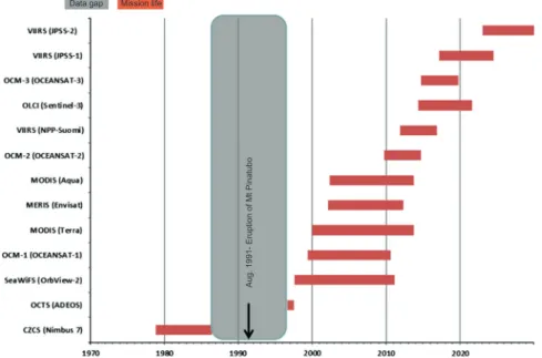
g/L. (For interpretation of the references to colour in this figure legend, the reader is referred to the web version of this article.)Data gap Mission life
Aug. 1991
-Eruption of Mt Pinatubo
Fig. 4.Timeline 1970–2030 illustrating past, current, and future global ocean-color satellite missions. Missions after 1999 were extracted from the online CEOS Earth Observation Handbook (http://www.eohandbook.com/). Satellite platforms are indicated. (For interpretation of the references to colour in this figure legend, the reader is referred to the web version of this article.)
Table 1
Detecting algal blooms from ocean color remote sensing: applications overview (cited research from 2006 to 2013 is indicative only).
Research application Global scale Local scale
Spatial and temporal distributions (phenology) Gower and King (2011a), Gower et al. (2008), Demarcq et al. (2012) and Racault et al. (2012)
Park et al. (2010b), Garcia and Garcia (2008), Gower and King (2007a), Song et al. (2010), Platt and Sathyendranath (2008), Henson et al. (2009)
Derivation of long terms baseline, and marine ecosystem’s response to i.e., climatic, anthropogenic forcing
Martinez et al. (2009) and Siegel et al. (2013)
Kahru et al. (2010), Shi and Wang (2007) and Zhao et al. (2008)
Ecosystem partitioning IOCCG (2009), Oliver and Irwin (2008) and Platt et al. (2008)
Henson et al. (2006)
Coastal zone management (eutrophication, etc.) Smetacek and Cloern (2008) Penaflor (2007), Banks et al. (2012), Klemas (2011) Biogeochemistry (carbon, nitrogen fluxes, etc.) Platt et al. (2008) Chang and Xuan (2011) and Focardi et al. (2009) Major phytoplankton groups (Coccolithophores,
Trichodesmium, etc.)
Moore et al. (2012) Carvalho et al. (2011), Miller et al. (2006), Shutler et al. (2012), McKinna et al. (2011) and Gower and King (2011b)
Size-class, community composition and physiology
Brewin et al. (2011), Behrenfeld et al. (2009)and
Pan et al. (2012, 2013) Extremes (e.g., super-blooms) Gower and King (2011a) Gower and King (2007a)
Table 2
Spectral bands (in nm) used in algal bloom indices for SeaWiFS, MODIS and MERIS (cited research is indicative only). Sensor Product Band 1 Band 2 Band 3 Algal bloom type References MODIS FLH 667 678 746 Algal blooms, surface algal blooms Hu et al. (2005)
MERIS FLH 665 681 708.75 Algal blooms Gower et al. (2003)
MODIS FAI 667 859 1240 or 1640 Surface algal blooms Hu (2009) SeaWiFS CIA 443 555 670 Low Chlorophyll concentrations Hu et al. (2012) MERIS MCI 681 708.75 753 High concentration in water and surface algal blooms Gower et al. (2003) MERIS MCIwide 665 708.75 753 High concentration in water and surface algal blooms Gower et al. (2004) MERIS EBI 665 708.75 n/a Surface algal blooms (Not peer-reviewed) Amin, R.
SeaWiFS RI 443 510 555 Algal blooms Ahn and Shanmugam (2006)
SeaWiFS ABI 443 490 555 HAB, algal blooms Shanmugam (2011) and Ahn and Shanmugam (2006) MODIS ABI 443 490 555 HAB, algal blooms Shanmugam (2011) and Ahn and Shanmugam (2006) MODIS KBBI & RBD 667 678 n/a Surface algal blooms (K. brevis) Amin et al. (2009b)
MERIS KBBI & RBD 665 681 n/a Surface algal blooms (K. brevis) Amin et al. (2008)
3.2. Reflectance band-ratio algorithms
In open ocean Case 1 waters, phytoplankton is the primary
water constituent (Morel, 1980; Morel and Prieur, 1977); thus,
Chl-a concentrations can be empirically related to the
water-leaving reflectance using relationships of various forms (e.g.,
Matthews, 2011; Dierssen, 2010). These empirical relationships
are often derived using large, sometimes global (e.g.,
Fargion and
McClain, 2003),
in situ
datasets of coincident Chl-a and reflectance
measurements. Empirical blue–green (440–550 nm) spectral
band-ratios are the most common types of ocean color algorithms used
for Chl-a retrievals because most of the phytoplankton absorption
occurs within this portion of the visible spectrum. However, the
use of visible wavelengths can be unreliable in coastal waters.
In optically complex, Case 2 waters, blue–green reflectance
band-ratios become less sensitive to changes in Chl-a concentrations
because increasing concentrations of color dissolved organic matter
(CDOM) and total suspended matter (TSM) (e.g.,
Bowers et al.,
1996) require the use of other spectral bands located in the
red (620–700 nm) and NIR (>700 nm) (e.g.,
Gitelson et al., 2009)
(Fig. 5).
3.2.1. Blue–green band-ratios for open and coastal ocean waters
Gordon et al. (1983, 1980)
and
Feldman et al. (1984)
were
among the first to use empirical band-ratios from CZCS spectral
bands for the study of the near-surface distribution of
phytoplank-ton blooms in the open ocean and to explore their relationships
with oceanographic conditions. Many other studies used their
ini-tial work to derive global phytoplankton maps from CZCS Chl-a
imagery (e.g.,
Banse and English, 2000, 1997, 1994; Nezlin et al.,
1999; Tang et al., 1999; Fuentes-Yaco et al., 1997b). The second
and third generation of ocean color sensors (Fig. 4; Fig. 5; see
Table 3Detecting phytoplankton blooms with CZCS (cited research is indicative only). Phytoplankton type Reflectance classification (thresholds, anomalies)
Reflectance band-ratios Bio-optical model or neural network Spectral band difference
Satellite product (threshold or anomaly) and climatology, statistics
Phytoplankton bloom (undefined)
Banse and English (2000), Kim et al. (2000), Yoder et al. (2001), Shevyrnogov et al. (2002b), Robinson et al. (2004) and Tang et al. (2004)
Banse and English (1999), Shevyrnogov et al. (2002a), Marinelli et al. (2008) and Antoine et al. (2005)a
Surface expression (undefined)
Coccolithophores Merico et al. (2003) Trichodesmium
Red tides/HAB a
Merged with SeaWiFS.
Table 4
Detecting phytoplankton blooms with SeaWiFS (cited research is indicative only). Phytoplankton type Reflectance classification (thresholds, anomalies)
Reflectance band-ratios Bio-optical model or neural network
Spectral band difference
Satellite product (threshold or anomaly) and climatology, statistics
Phytoplankton bloom (undefined)
Otero and Siegel (2004)
Gower (2001), Lavender and Groom (2001), Gohin et al. (2003), Santoleri et al. (2003), Thomas et al. (2003),
Vinayachandran and Mathew (2003), Claustre and Maritorena (2003), Babin et al. (2004), Otero and Siegel (2004), Ahn et al. (2005), Iida and Saitoh (2007)and Siegel et al. (2013)
Shanmugam (2011), Dierssen and Smith (2000) andSiegel et al. (2013)
Hu et al. (2012)
Saitoh et al. (2002), Nezlin and Li (2003), Srokosz et al. (2004), Brickley and Thomas (2004), Navarro and Ruiz (2006), Tan et al. (2006), Henson and Thomas (2007), Marrari et al. (2008), Yoo et al. (2008), Garcia-Soto and Pingree (2009), Henson et al. (2009), Platt et al. (2009) Quartly and Srokosz (2004), Vargas et al. (2009), Song et al. (2010), Raitsos et al. (2011), Racault et al. (2012) and Kidston et al. (2013) Surface
expression (undefined)
Coccolithophores Iida et al. (2002), Zeichen and Robinson (2004) andMoore et al. (2012) Trichodesmium Subramaniam
et al. (2002)and Dupouy et al. (2011)
Red tides/HAB Ahn et al. (2006)andTang et al. (2006) Stumpf (2001) Ahn and Shanmugam (2006)and Shanmugam et al. (2008)
Miller et al. (2006), Stumpf et al. (2003) and Tomlinson et al. (2004)
Table 5
Detecting phytoplankton blooms with MODIS (cited research is indicative only). Phytoplankton type Reflectance classification (thresholds, anomalies)
Reflectance band-ratios Bio-optical model or neural network
Spectral band difference
Satellite product (threshold or anomaly) and climatology, statistics Phytoplankton bloom (undefined) Venables et al. (2007)a , Shang et al. (2010), Shanmugam (2011)andMélin et al. (2011)a
Hu et al. (2012) Wang and Zhao (2008)a
,Shi and Wang (2007), Uz (2007)a
,Peñaflor et al. (2007), White et al. (2007)a
, Oliveira et al. (2009), Park et al. (2010a, 2010b), Raj et al. (2010)a ,Wang et al. (2010)a ,Li et al. (2010b) and Acker et al. (2008)a ,Zhao et al. (2009a)a,Kahru et al. (2010)a,b,
Nezlin et al. (2010)a andLe et al. (2013) Dasgupta et al. (2009) Surface expression (undefined)
Coccolithophores Signorini and McClain (2009), Balch et al. (2005) Iida et al. (2012)and Moore et al. (2012) Trichodesmium McKinna et al.
(2011)
Hu et al. (2010a) Red tides/HAB Siswanto et al.
(2013)
Kahru et al. (2004)and Carvalho et al. (2011) Cannizzaro et al. (2008)a and Carvalho et al. (2010) Hu et al. (2005), Ryan et al. (2009) andZhao et al. (2010)b
Cannizzaro et al. (2008), Cannizzaro (2004), Hu et al. (2004), Tomlinson et al. (2008)a
,Anderson et al. (2011), Banks et al. (2012)a
,Shutler et al. (2012)andKurekin et al. (2014)b
a Merged with SeaWiFS. b Merged with MERIS.
Table 6
Detecting phytoplankton blooms with MERIS (cited research is indicative only). Phytoplankton type Reflectance classification
(thresholds, anomalies)
Reflectance band-ratios
Bio-optical model or neural network
Spectral band difference Satellite product (threshold or anomaly) and climatology, statistics Phytoplankton bloom
(undefined)
Uiboupin et al. (2012) Gower et al. (2008, 2005) Gordoa et al. (2008) Surface expression
(undefined)
Gower and King (2011a) Coccolithophores Moore et al. (2012)
Trichodesmium Matthews et al. (2012)
Red tides/HAB Bernard et al. (2005) Ryan et al. (2008)and
Jessup et al. (2009) Li et al. (2010a)
VIIRS
CDOM, Turbidity Chl Pigments Turbidity, TSM TSM Chl & red-edge Fluorescence Atmospheric correctionFig. 5.Comparison of the spectral band positions for five ocean color sensors of the first (CZCS), second (SeaWiFS), third (MERIS, MODIS) and fourth (VIIRS) generations. (Figure modified from Fig. 1 ofLee et al. (2007). The authors used 14 remote sensing reflectance spectra from various waters around the world. The potential applications for each spectral region are indicated. SeeTable 2as well (this review.) (For interpretation of the references to colour in this figure legend, the reader is referred to the web version of this article.)
Fig. 3 of
Klemas (2012)) addressed the need for more spectral
bands, thereby enabling the development of more sophisticated
atmospheric correction schemes and in-water constituent retrieval
algorithms, which are required for both improved retrieval
accu-racy for water quality variables and algal bloom proxies in coastal
ocean waters. SeaWiFS OC4 (O’Reilly et al., 2000, 1998) and MODIS
OC3M (Campbell and Feng, 2005b, 2005a) are switching band-ratio
algorithms that use spectral bands in the blue and green regions of
the visible spectrum to estimate Chl-a concentrations. The MODIS
OC3M (e.g.,
Chen and Quan, 2013) is extended from the SeaWiFS
OC4 and adapted to the MODIS spectral bands. The use of global
standard ocean color band-ratios has been demonstrated to
signif-icantly overestimate Chl-a.
Moore et al. (2009)
have shown that
the nominal uncertainty of 35% for Chl-a retrievals is true in ocean
gyres, but the OC3M relative Chl-a error is >50%outside those gyres
and can be >100% in coastal waters.
Komick et al. (2009)
found that
MODIS OC3M systematically overestimated Chl-a when lower than
0.13 mg m
3in Western Canadian waters. Similar results were also
found by
Radenac et al. (2013)
for the equatorial Pacific warm pool.
For SeaWiFS OC4,
Volpe et al. (2007)
found that Chl-a was
overes-timated by 70% for Chl-a levels lower than 0.2 mg m
3in the
Med-iterranean Sea. Such low Chl-a concentrations are encountered in
the vast majority of the global ocean (Hu et al., 2012).
3.2.2. The relevance of the red-NIR spectral regions in coastal waters
The
in vivo
absorption peak near 676 nm is minimally affected
by the influence of CDOM and TSM when the two are in low
con-centrations (see Section
3.3;
Fig. 5). Spectral bands near 676 nm
have been widely used for the retrieval of Chl-a in coastal waters
(Odermatt et al., 2012; Gurlin et al., 2011).
Gitelson et al. (1999)
have shown that reflectance increases in the NIR beyond 700 nm
due to increased scattering from algal biomass, correlated to an
in-crease in Chl-a for most phytoplankton groups. The sensitivity
analysis conducted by
Ruddick et al. (2001)
on two red-NIR
band-ratio algorithms revealed that the relative error on Chl-a
ret-rievals became more significant at low Chl-a concentrations
(<10 mg m
3) and in low backscatter conditions but also that the
choice of paired wavelengths was very important. Their study
showed that a band-ratio algorithm that uses the red-NIR band
pair 672 and 704 nm would perform best at Chl-a
10 mg m
3,
whereas a wider red-NIR band pair spreading further apart (e.g.,
667 and 748 nm) would perform best at Chl-a
100 mg m
3.
The ‘‘red-edge’’ is technically defined as an increase in spectral
reflectance in the red-NIR (680–750 nm) and often results from the
presence of partly submersed vegetation (e.g.,
Dierssen et al., 2007,
2006; Bostater et al., 2003; Gitelson, 1992) or algal bloom surface
expressions (e.g.,
Shen et al., 2012; Ruddick et al., 2008) (Fig. 5).
Only a few ocean color sensors have the spectral requirements that
enable the detection of those reflectance features. For SeaWiFS,
two of the nine spectral bands are positioned in red-NIR region
of the spectrum (namely 670 nm and 765 nm), and these two
bands have limited use for the detection of Chl-a. In contrast,
MODIS and MERIS provide more spectral bands between 600 and
800 nm (Figs. 5 and 6). Further useful applications of the red-NIR
spectral region in reflectance-based algorithms are discussed in
Sections
3.3 and 4.
3.2.3. Band-ratio algorithms: Limitations and challenges
Most reflectance band-ratios are designed for global
applica-tions over optically deep ocean waters (Odermatt et al., 2012).
The use of band-ratios often leads to erroneous retrievals in coastal
waters, where the optical complexity is highly variable (Dierssen,
2010; Blondeau-Patissier et al., 2004). Additional limitations in
the use of band-ratios are regional differences in optical properties
and concentrations; the generalized global parameterization of
some algorithms is inapplicable in some of the world’s ocean
regions (e.g.,
Volpe et al., 2007; Claustre and Maritorena, 2003;
Sathyendranath et al., 2001; Dierssen and Smith, 2000). Many
studies have shown that the retrieval accuracy of Chl-a by satellite
ocean color sensors, aimed to be within ±35% in oceanic waters,
cannot always be met when using band-ratio algorithms (e.g.,
Moore et al., 2009; Hu et al., 2000). In coastal waters, the quality
of this retrieval significantly degrades and is often considered
unreliable. The use of blue–green spectral bands for the specific
detection of Chl-a in coastal waters is affected by the absorption
signal of CDOM and TSM (e.g.,
Dierssen, 2010; Gower, 2000;
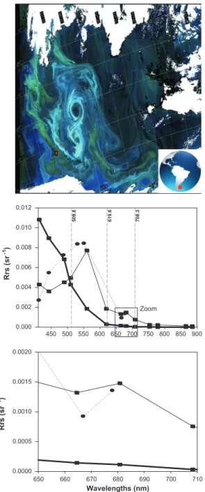
Wavelengths (nm) 450 500 550 600 650 700 750 800 850 900 Rrs (sr -1) Rrs (sr -1) 0.000 0.002 0.004 0.006 0.008 0.010 0.012 650 660 670 680 690 700 710 0.0000 0.0005 0.0010 0.0015 0.0020 Zoom 509.8 619.6 708.3
Fig. 6.Detecting algal blooms from MODIS and MERIS ocean color sensors. Top panel: RGB MERIS image of December 2, 2011 showing the pixel location (red dot) for the extracted reflectance data; middle panel: remote sensing reflectance spectra (Rrs) of MERIS (thin line) and MODIS (dotted line) Level 2 (standard algorithms) for the same day. Reflectance from the surrounding blue water is shown (thick line); bottom panel: zoom on the spectral region 650–710 nm. MERIS bands at 509.81, 619.30 and 708.32 nm are shown by vertical dashed lines. (For interpretation of the references to colour in this figure legend, the reader is referred to the web version of this article.)
Joint and Groom, 2000). To overcome this limitation, other studies
suggested the use of red-NIR band-ratios for Chl-a retrieval in
coastal waters (e.g.,
Moses et al., 2012; Shanmugam, 2011).
3.3. Spectral band difference algorithms
Spectral band difference algorithms exploit spectral regions
that feature significant changes in the reflectance spectrum due
to the presence of an algal bloom, compared to the nearby
bloom-free water. Given that absorption tends to vary more
rap-idly with wavelength than scattering, two adjacent reflectance
spectral bands may have similar backscattering properties but will
differ significantly in absorption. Hence, this absorption feature
can be quantified by spectral difference. The various forms of
spec-tral band difference algorithms use band triplets from the red-NIR
or the blue–green spectral regions (Table 2) depending on whether
the algorithm is designed to be sensitive to an algal group, high
chlorophyll concentrations or surface bloom expressions (Fig. 7).
One of the most used ocean color spectral band difference
algo-rithms is the Fluorescence Line Height (FLH) (see review of
et al. (2007)), an index for quantifying solar-induced chlorophyll
fluorescence. Other similar mathematical expressions are used to
derive algal bloom indices from SeaWiFS, MERIS and MODIS
(Table 2) and are discussed in this section.
3.3.1. Fluorescence Line Height (FLH)
The literature published on this topic since the 1960s (Yentsch
and Menzel, 1963) has shown that estimating fluorescence is
greatly beneficial to studies of phytoplankton biomass (Falkowski
and Kiefer, 1985), physiology (e.g.,
Westberry et al., 2013;
Behren-feld et al., 2009), and composition (e.g.,
Hu et al., 2005). The remote
sensing approach used to retrieve FLH was originally developed by
Neville and Gower (1977), and its first application to an ocean color
sensor was on MODIS-Terra (Abbott and Letelier, 1999; Letelier
and Abbott, 1996). It is well known, however, that MODIS-Terra
suffers from uncertainties and instabilities, particularly the
radio-metric response of the 412-nm band, which has significantly
(>40%) degraded since the start of the mission (Franz et al.,
2008). The significant striping in MODIS-Terra water-leaving
radi-ances makes the data largely unusable. Thus, MODIS mostly refers
to the sensor on the Aqua satellite. The spectral band positions of
MERIS (Gower et al., 1999) and MODIS (Hoge et al., 2003) allow
Fig. 7.The Algal Bloom Index (ABI) is used to map phytoplankton blooms in the Arabian Sea and the Gulf of Oman from a MODIS-Aqua scene of February 28, 2010. Fig. 4 from Shanmugam (2011). Top panel: A MODIS/Aqua true color composite on 18 February 2010 in the Arabian Sea and Gulf of Oman; The corresponding Chl-a images are derived using (middle) the OC3 and (bottom) ABI algorithms.
for the computation of FLH, but this product cannot be derived
from CZCS, SeaWiFS and VIIRS because of the lack spectral bands
in the 670–690 nm range.
Gower and Borstad (2004)
and
Zhao
et al. (2010)
compared FLH results between MODIS and MERIS
and concluded that MERIS bands were better positioned for
mea-suring fluorescence. The use of MODIS FLH to detect HAB has been
successfully used by many (Frolov et al., 2013; Cannizzaro et al.,
2008; Hu et al., 2005), providing more reliable information than
a standard Chl algorithm. MERIS FLH was found to be successful
at detecting high biomass phytoplankton in sediment-dominated
coastal waters (e.g.,
Gower et al., 2005). However, others studies
have led to inconclusive results on the benefits of FLH in the
detec-tion of algal blooms (e.g.,
Tomlinson et al., 2008).
3.3.2. Maximum Chlorophyll Index (MCI)
The Maximum Chlorophyll Index (MCI) can only be applied to
MERIS because of its use of the 708.75 nm band. This band is more
responsive to strong reflectance in the NIR, and the lack of similar
bands in MODIS and VIIRS may hamper the detection of
high-concentration bloom events. The MCI is mainly designed for the
detection of high-concentration algal blooms, and it was
successfully used to globally monitor phytoplankton blooms in
the world’s oceans by
Gower et al. (2008). The minimum Chl-a
concentration required for a phytoplankton bloom to be detected
by the MCI is
30 mg m
3(Gower et al., 2005), but phytoplankton
blooms can have much higher concentrations, with some studies
reporting Chl-a > 200 mg m
3(e.g.,
Gower and King, 2007a;
Sasamal et al., 2005).
3.3.3. Floating Algae Index (FAI) and Scaled Algae Index (SAI)
Hu et al. (2010c) and Hu (2009)
proposed the Floating Algae
In-dex (FAI) to detect large (>4000 km
2) surface-floating algae from
MODIS 250 and 500 m bands in both fresh and marine
environ-ments. The FAI uses a functional form similar to FLH and MCI
where the height of the NIR peak is estimated relatively to a linear
baseline from adjacent bands in the red and short wave infrared
(SWIR) wavelengths (Table 2). Thus, the FAI is sensitive to the
red-edge and is robust to the influence of CDOM, aerosols and
sun glint because of the use of NIR bands. However, similarly to
MCI, the FAI is likely sensitive to turbid waters and shallow depths.
It is used in combination with pre-determined thresholds to help
separate land, cloud and high concentrations of submersed algae
or sediments from pixels associated with surface algae scums.
FAI was originally applied to the detection of cyanobacteria and
macro-algae in the freshwater lake Taihu and the Yellow Sea
(China). Its global applicability remains untested. Building on this
research,
Garcia et al. (2013)
developed an automatized image
processing algorithm, the Scaled Algae Index (SAI), which is a
necessary intermediate product for quantifying the spatial
coverage of the floating macro-algae observed in satellite imagery
based on FAI.
3.3.4. Color Index Algorithm (CIA)
A recent development in algal bloom indices is the Color Index
Algorithm (CIA) proposed by
Hu et al. (2012). This empirical
algorithm was originally developed to estimate surface Chl-a
concentrations in oligotrophic (
6
0.25 mg m
3) waters. The CIA is
a three-band reflectance difference algorithm (443 nm, 555 nm
and 670 nm bands), making it applicable to SeaWiFS, MODIS and
MERIS. Its accuracy has not yet been fully validated because of
the lack of low-concentration, high-quality
in situ
Chl-a data from
the world’s oceans. The CIA was successfully applied to the waters
of the Red Sea by
Brewin et al. (2013), where it was found to
per-form better than the MODIS OC3 at retrieving Chl-a because of the
low concentrations typically encountered in those waters.
3.3.5. Spectral band difference algorithms: Limitations and challenges
Many limitations in the use of red-NIR bands have been raised
in this section. The robust application of FLH for the detection of
algal blooms remains under discussion.
McKee et al. (2007)
sug-gested that the FLH signal could be masked in complex coastal
waters due to the influence of CDOM and TSM. Similarly,
Gilerson
et al. (2007, 2008)
found that MODIS FLH retrieved fluorescence
with reasonable accuracy only for waters with Chl < 4 mg m
3but that the signal was masked by particulate backscattering in
turbid waters with high CDOM and TSM concentrations. The
authors also questioned the performance of the MERIS FLH
algo-rithm in coastal waters where large errors could be introduced
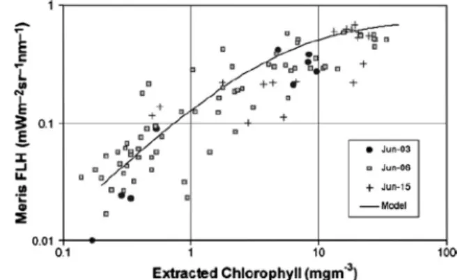
via the linear baseline between the 665 nm and 708.75 nm bands.
The use of a linear baseline between the two NIR MERIS bands for
the computation of FLH has been demonstrated to work in coastal
waters with Chl-a concentrations of up to 20 mg m
3(Gower and
King, 2007b) (Fig. 8). For higher chlorophyll concentrations
how-ever, due to the combined effects of water absorption and Chl-a
distortion, the Chl-a spectrum and a linear baseline can no longer
be used.
Gower et al. (1999)
also challenged the theory that the
scattering by TSM had a significant reducing effect on the relative
fluorescence height above the baseline. The influence of CDOM on
the FLH is often considered small in relatively low concentrations
due to its negligible absorption in the NIR.
Hu (2009)
acknowl-edged that limitations in the MODIS FAI included the questionable
reliability of the MODIS atmospheric correction and the lack of a
MODIS-cloud masking algorithm that would reliably flag all cloud
and/or sun-glint contaminated pixels while keeping (floating)
al-gae pixels. Although the first issue can be easily solved using
Ray-leigh-corrected reflectance (Hu et al., 2010b), the second remains a
problem, and the author suggested the use of true-color FAI-paired
images to separate the clouds from the ocean surface features.
Sev-eral ocean color algal bloom indices can be combined to enhance
our interpretation of algal bloom phenomena and their underlying
mechanisms (see Section
5.3).
3.4. Bio-optical models
Bio-optical models are based on various fundamental theories
of marine optics and, because they rest on firm theoretical bases
and rigorous equations, they are often robust (e.g.,
Morel, 2001).
Coastal systems are generally shallow (<100 m), dynamic,
transi-tional environments that receive considerable amounts of
freshwa-ter inputs carrying nutrients, dissolved and particulate organic
matter, sediment and contaminants (Blondeau-Patissier et al.,
2009; Babin et al., 2003). Extracting detailed and accurate
informa-tion from ocean color imagery is a more challenging task in coastal
Fig. 8.The MERIS FLH product as a function of surface extracted chlorophylls from the Canadian west coast, ECOHAB project, June–September 2003. Fig. 4 ofGower and King (2007b).
waters in comparison to the open ocean (Tilstone et al., 2011b; Qin
et al., 2007). Inversed modeling algorithms (Odermatt et al., 2012)
are often necessary to enable the accurate retrieval of Chl-a
concentrations in optically complex waters, although optically
ac-tive constituents (CDOM, TSM) may show discernible patterns of
their own during algal bloom conditions (e.g.,
Chari et al., 2013;
Zhao et al., 2009b).
3.4.1. Retrieval of taxa-specific pigment concentrations from
bio-optical models
Taxonomic phytoplankton groups contain different
combina-tions of pigments (e.g.,
Uitz et al., 2006), but the spectral features
of individual pigments are often similar (e.g.,
Aiken et al., 2008;
Richardson, 1996). There is still some debate about which
phyto-plankton pigments can be reliably identified because many water
quality parameters confine the algorithms to specific conditions.
However, the use of the (specific) absorption coefficient of
phyto-plankton indexed to the composition of the phytophyto-plankton
com-munity sampled
in situ
has brought promising results in open
ocean waters (e.g.,
Claustre et al., 2005; Sathyendranath et al.,
2004). Such techniques are employed to detect phytoplankton
community structures from ocean color datasets (e.g.,
Brewin
et al., 2011), but significant progress is yet to be made, both in
the bio-optical models and databases, for their use in coastal
waters.
3.4.2. Derivation of inherent optical properties from bio-optical models
for the detection of algal blooms
The principal phytoplankton pigments that mostly contribute to
absorption are the photosynthetic pigments consisting of the
chlo-rophylls, carotenoids and biliproteins. The phytoplankton
absorp-tion coefficient is an important parameter in ocean color
algorithms and is increasingly used to parameterize algal bloom
algorithms (e.g.,
Goela et al., 2013). To study the phytoplankton
dynamics characterizing the coastal waters of the Taiwan Strait,
Shang et al. (2010)
used the Quasi-Analytical Algorithm (QAA)
from
Lee et al. (2002)
to retrieve the phytoplankton absorption
coefficient from MODIS. Their findings promoted the use of the
phytoplankton absorption coefficient over Chl-a because the latter
can suffer from the contamination of non-biotic optically active
material.
3.4.3. Bio-optical models: Limitations and challenges
Bio-optical forward and inverse modeling is developing rapidly
as an essential tool to understand the effects of dense algal
concen-trations on light absorption and backscattering coefficients. False
positive bloom detections in CDOM- or TSM-rich waters and
uncertainties due to the quality of the atmospheric correction are
still hampering accurate retrievals of optical properties and
bio-geochemical concentrations in coastal waters. The use of specific
inherent properties now has a central role in bio-optical modeling
(e.g.,
Brando et al., 2012; Tilstone et al., 2011a), but the
identifica-tion of specific phytoplankton groups on the basis of inherent
opti-cal properties remains a challenge in coastal waters. For future
parameterizations of taxa-specific bio-optical models,
Claustre
et al. (2005)
stressed the need to make coincident measurements
of the phytoplankton taxonomic composition, photophysiological
parameters and phytoplankton absorption to improve local,
regio-nal and global
in situ
databases. As suggested by
Dierssen (2010)
and later by
Sen Gupta and McNeil (2012), the water properties
of the world’s oceans are changing. It is probable that algorithm
parameterizations derived from
in situ
data collected over the past
decades might not be applicable in the near future due to the
pos-sible change in the CDOM–Chl relationships in coastal waters. One
of the latest reports on future ocean color mission requirements,
IOCCG Report 13 (2012b), stated that ‘‘
phytoplankton blooms’
timing, frequency, composition and intensity are expected to change
with climate in ways that may be hard to predict. (
. . .
). Thus reliable
and accurate detection of algal blooms is an objective for future
missions
’’ (p. 14).
4. The detection of specific types of algal blooms
4.1. Algal blooms with surface expressions
Algal blooms with surface expressions, such as occolithophores,
cyanobacteria and
Sargassum
, are observable in satellite imagery
due to the large areas they often cover (Fig. 1). Spectral
character-istics specific to those taxa may be exploited for their mapping, or
masking, by using empirically derived, rule-based reflectance
clas-sification algorithms; bio-optical models can also be used.
4.1.1. Coccolithophore blooms
Coccolithophores, with the globally dominant
Emiliania huxleyi
,
are calcifying phytoplankton species that form large, dense blooms
occurring at most latitudes (Brown, 1995). Coccolithophore blooms
play an important role in ocean biogeochemistry (Harlay et al.,
2011) and the upper ocean light field (e.g.,
Balch et al., 2005).
The senescent stage of Coccolithophore blooms is often identifiable
in an ocean color remote sensing image by its milky blue–green
color (Fig. 1), accompanied by the typical high scattering across
all spectral bands (400–800 nm) that results from the detached
coccoliths (Voss et al., 1998). Following the early work of
Holligan
et al. (1983), who reported on the higher reflectance values found
for CZCS satellite image pixels within Coccolithophore-rich waters,
Brown and Yoder (1994a)
and
Brown (1995)
pioneered research on
the detection of Coccolithophore blooms. Using a reflectance
clas-sification technique to map those events in the global ocean,
Brown and Yoder (1994a), Ackleson et al. (1994)
and, later,
Merico
et al. (2003)
identified many limitations that were associated with
this technique, including false positives resulting from various
sources, such as poor satellite coverage, atmospheric correction
er-rors, reflectance signal contamination from CDOM and scattering
from resuspension of TSM. These contaminating sources, whether
individual or combined, could bias the results obtained not only
for the detection of Coccolithophore blooms but also those of
Chl-a (e.g.,
Blondeau-Patissier et al., 2004). Nonetheless, the
acceptable accuracy of the classification results led to the
docu-mentation of Coccolithophore bloom events at both global (e.g.,
Brown, 1995) and basin scales (e.g.,
Brown and Podesta, 1997;
Brown and Yoder, 1994b). Since this early work with CZCS
(Ta-ble 3), novel methods have been developed using reflectance
anomalies (e.g.,
Shutler et al., 2010) and reflectance classifiers
(e.g.,
Moore et al., 2012) with SeaWiFS (Table 4), MODIS (Table 5)
and MERIS (Table 6). These new approaches allowed for the
map-ping of Coccolithophore blooms in ocean regions where previously
such blooms were either not detected or underestimated, such as
shelf or polar seas (e.g.,
Holligan et al., 2010; Hegseth and
Sundfj-ord, 2008). The use of existing standard Coccolithophore masks in
those regions is often unsuitable, and some regional adjustments
are required.
Iida et al. (2002)
demonstrated that the thresholds
used in the NASA standard SeaWiFS Coccolithophore mask
algo-rithm were too high to map the events in the Bering Sea and lower
threshold values were necessary.
4.1.2. Trichodesmium blooms
Blooms of cyanobacterium
Trichodesmium
fix atmospheric
nitrogen into ammonium, making it usable for other organisms
(e.g.,
LaRoche and Breitbarth, 2005).
Subramaniam and Carpenter
(1994)
qualitatively mapped
Trichodesmium sp
. blooms from CZCS
satellite imagery of the Atlantic, Indian and Pacific Oceans using an
Please cite this article in press as: Blondeau-Patissier, D., et al. A review of ocean color remote sensing methods and statistical techniques for the detection,empirical reflectance algorithm based on their high reflectivity.
Due to the strong absorption by phycoerythrin,
Trichodesmium
blooms have a characteristic spectral feature at 550 nm that makes
them potentially identifiable in satellite reflectance spectra.
Bio-optical properties specific to
Trichodesmium
were also used by
Subramaniam et al. (1999a,b)
for the large-scale detection of such
events in AVHRR imagery off the Somali coast from a
reflectance-based model. Those properties were subsequently used in a
semi-empirical bio-optical model by
Subramaniam et al. (2002)
to detect
Trichodesmium
events in SeaWiFS imagery off the South
Atlantic Bight, demonstrating that
Trichodesmium
blooms could
be detected in optically complex coastal waters when in sufficient
quantity. However, this model had some limitations, including
sensitivity to bottom reflection and corals and generating false
positives from other similarly reflective sources (such as
Cocco-lithophore or
Phaeocystis
blooms, TSM). Recent studies employ
criterion-based reflectance techniques to detect and quantify
Trichodesmium
floating mats using reflectance anomalies (Dupouy
et al., 2011, 2008), high-resolution NIR bands (McKinna et al., 2011)
and blue–green reflectance bands with MODIS.
Hu et al. (2010a)
demonstrated the potential of MODIS FAI to distinguish
Trichodesmi-um
mats from the background influence of both TSM and CDOM in
the coastal waters of Florida, on the condition that
Trichodesmium
was in sufficiently high concentration (i.e., Chl-a > 4 mg m
3). Mostly
a qualitative approach (e.g., presence/absence), very few of these
reflectance-based studies provide quantitative estimates of
Trichodes-mium
blooms from satellite imagery. The quantitative estimate of
Trichodesmium sp.
abundances can be achieved with the use of
taxa-specific pigment retrieval models.
Westberry et al. (2005)
used
an extension of the bio-optical model of
Garver and Siegel (1997)
and
Maritorena et al. (2002)
(GSM) to map the abundance and
biomass of
Trichodesmium
on a global scale from SeaWiFS imagery.
These two studies helped reveal many aspects of the distribution of
Trichodemsium sp.
in the global ocean, with the largest annual
spatio-temporal occurrence of
Trichodesmium sp
. in the Pacific Ocean.
4.1.3. Floating Sargassum
Sargassum sp.
are surface-floating macro-algae distributed
throughout the temperate and tropical oceans.
Sargassum
some-times cover large areas (tens of kilometers), which may provide a
useful proxy for tracking convergent or divergent oceanographic
processes (e.g.,
Zhong et al., 2012). MERIS MCI and MODIS FLH
have been shown to be very effective in monitoring their
distribu-tions in the Gulf of Mexico and the North Atlantic Ocean (Gower
and King, 2011b, 2008; Gower et al., 2006). Using those surface
expression indices,
Gower and King (2011b)
have shown that
Sargassum sp.
seasonal occurrences are characterized by a
migra-tion from the Gulf of Mexico in spring to the North Atlantic in July,
ending near the Bahamas in February of the following year. An
estimated biomass of floating
Sargassum
of 1 g Chl kg
1wet algae
(Gower et al., 2006) corresponds to 10
6ton yr
1sourced from
the Gulf of Mexico, which may have large implications for
carbon fluxes (Gower and King, 2011b). The spatial and seasonal
distributions of
Sargassum
have, overall, been well mapped using
satellite imagery, but
Gower et al. (2013)
recently showed a large
drift in their distributions for the year 2011, the cause of which
is unclear.
4.1.4. Harmful Algal blooms – Example of dinoflagellate Karenia brevis
The outbreak of a single, dominating phytoplankton species can
alter coastal ecosystems, often causing costly damages to both the
local economy and the marine ecosystem (e.g.,
Babin et al., 2008;
Hu et al., 2004). Harmful algal blooms are often referred to as
red tide events, but a reddish appearance of the ocean water can
be caused by any phytoplankton species, with the only variable
being its concentration (Kutser, 2009; Dierssen et al., 2006).
Red-tide-type phytoplankton species, such as dinoflagellate
Kare-nia brevis
, absorb radiations in the blue and lower green regions
(450–500 nm) of the visible spectrum while strongly reflecting
radiations in the yellow region (570–580 nm).
Bernard et al.
(2005)
used an empirical Chl-a algorithm based on the ratio
be-tween the MERIS red bands 665 and 709 nm to detect high biomass
(up to 200 mg m
3) dinoflagellate-dominated HAB events in the
Southern Benguela. Another band-ratio was proposed by
Ahn and
Shanmugam (2006). The Red Tide Index (RI) is specifically
de-signed to detect red-tide blooms (Table 2). The Red Tide Index
Chlorophyll Algorithm (RCA) empirically relates RI to Chl-a for
con-centrations of up to 70 mg m
3(see Fig. 6 from
Ahn and
Shanmu-gam (2006)). Their findings showed that spatial patterns of
red-tide blooms as mapped from the RI and RCA indices were more
consistent with field observations than when standard band-ratio
algorithms were used. In this case,
Ahn and Shanmugam’s (2006)
study demonstrated the successful application of the band-ratio
approach over bio-optical models such as the one developed by
Cannizzaro et al. (2008)
for the Gulf of Mexico from SeaWiFS and
MODIS imagery. Band difference algorithms are also used. The
Red Band Difference (RBD) proposed by
Amin et al. (2009a,
2009b)
is an index specifically designed to detect
K. brevis
. The
spectral region used for the RBD (665–681 nm) is sensitive to both
phytoplankton absorption and scattering from suspended
sedi-ment; thus, an additional discrimination algorithm is required,
the
Karenia brevis
Bloom index (KBBI) (Amin et al., 2008;
Table 2).
KBBI is the ratio of the RBD to the sum of the same two normalized
water reflectance bands. This procedure can be applied to both
MODIS and MERIS and has been demonstrated to work in waters
other than the Gulf of Mexico (e.g., Gulf Stream, mid-Atlantic).
5. Statistical techniques and data assimilation to assess
phytoplankton bloom dynamics
The mapping of the seasonal, inter-annual, or decadal cycle of
phytoplankton growth, which can include its spatial patterns,
tim-ing and magnitude, is key to understandtim-ing algal bloom dynamics
in a specific ocean region. The sole use of an ocean color dataset is
often insufficient for accurately resolving ocean color constituents
(e.g.,
Mélin et al., 2011; Zingone et al., 2010; Uz, 2007), and
addi-tional data sources from models (e.g.,
Mouw et al., 2012) or
non-ocean color satellite sensors (e.g.,
Robinson et al., 2004; Saitoh
et al., 2002)can be necessary. In addition, statistical techniques
are often used as a post-processing step to unravel the temporal
and/or spatial patterns of those events (e.g.,
Kurekin et al., 2014).
The comprehensive reviews of
Bierman et al. (2011)
and
Kitsiou
and Karydis (2011)
already described the univariate and
multivar-iate statistical techniques that can be applied to water quality data.
Klemas (2012)
and
Brody et al. (2013)
used case studies to
illus-trate the applications of remote sensing techniques for the
detec-tion of phytoplankton blooms. This secdetec-tion provides addidetec-tional
material to these reviews and explores the various statistical
tech-niques that can be employed to extract further information from
satellite-derived climatologies and time-series.
5.1. Statistical partitioning of marine ecosystems
To analyze the dynamics of phytoplankton blooms in a study
re-gion, it is often necessary to first partition it into sub-regions
(IOCCG Report 9, 2009). The fundamental difference between the
partition of terrestrial and aquatic ecosystems is that aquatic
ecosystems usually have dynamic boundaries between biomes
to account for seasonal or inter-annual variations (Platt and
Sathyendranath, 1999).
Longhurst (1995)
was among the first to
provide a classification of the oceanic pelagic environment based
Please cite this article in press as: Blondeau-Patissier, D., et al. A review of ocean color remote sensing methods and statistical techniques for the detection,on the spatial variability of the ocean’s physical properties. Other
work has followed using satellite-derived Chl-a as the main
vari-able to characterize the spatial distribution, areal extent and
dynamics of phytoplankton blooms using multivariate statistical
analysis (e.g.,
Brickley and Thomas, 2004; Fuentes-Yaco et al.,
1997a).
Hardman-Mountford et al. (2008)
used six years of
SeaW-iFS Chl monthly global composites and Principal Component
Anal-ysis (PCA) to characterize broad-scale ecological patterns in the
world’s oceans. Their classification, based on the Chl spatial
distri-bution and variability, was consistent with Longhurst’s grouping of
four primary biomes, although a major difference emerged for the
equatorial biome. The delineation of ecosystem boundaries can be
performed using clustering methods (e.g., K-means and Empirical
Orthogonal Functions) to describe the spatial and temporal
vari-ability of a study region (e.g.,
Bergamino et al., 2010; Henson and
Thomas, 2007; Brickley and Thomas, 2004) (Fig. 9).
5.2. Time-series, fitted models and signal processing techniques
The statistical analysis of algal biomass cycles using time-series
can help detect trends in a dataset or reveal correlations between
the dynamics of phytoplankton biomass and environmental factors
that may be inherent to a study region.
A special issue of the journal Estuaries and Coasts (Zingone
et al., 2010) was dedicated to the analysis of multi-scale
phytoplankton variability for 22 coastal ecosystems around the
world by means of 84 timeseries, some of which were computed
from remote sensing data. This special issue highlighted the power
of time-series analysis as a statistical technique for deriving
environmental baselines. Although SeaWiFS, MODIS-Aqua and
MERIS individually have at least a decade of ocean color data,
multiple-sensor data merging is often required to significantly
extend the timeseries.
Maritorena et al. (2010)
showed that over
a seven year-period, the average daily coverage of the world’s
ocean was
25% when a merged satellite product was used, almost
double the global coverage of any single mission.
Kahru et al.
(2010)
merged data from SeaWiFS, MERIS and MODIS-Aqua to
examine the timing of the annual phytoplankton bloom maximum
in the Arctic. The data merging of satellite-derived surface Chl-a
extended their time series as far back as 1997 (Tables 1 and 5).
The authors found significant trends towards earlier phytoplankton
blooms in
11% of their study area.
The analysis of timeseries can be approached using
time-domain methods or mixed time-and frequency-time-domain methods.
The first technique analyzes data series in the same space in which
they were observed, whereas the second decomposes data series at
different time scales and frequencies. The sole use of
frequency-domain approaches for time-series analyses of phytoplankton
biomass is not common. In the timedomain, the timeseries is
decomposed into individual, periodic oscillations, the sum of
which matches the original signal.
Platt et al. (2009)
and
Song
et al. (2010)
qualitatively analyzed the timeseries of SeaWiFS data
of Chl-a for 10 regions of the Northwest Atlantic Ocean over a
10-year period (1998–2007) with a time-domain approach. To
quantify the timing of the spring and summer blooms, they fitted
a shifted-Gaussian model to the satellite-derived chlorophyll data
using a non-linear least-squares method. They found that blooms
in some regions occurred consistently earlier than their expected
latitudinal norm.
Mixed time–frequency statistical techniques include the
Empir-ical Mode Decomposition (EMD) (Huang et al., 1998), a signal
pro-cessing technique that is datadriven and decomposes an initial
signal into several high- and low-frequency oscillation
compo-nents, or wavelets (e.g.,
Demarcq et al., 2012; Nezlin and Li,
Fig. 9.Use of multivariate statistical analysis and satellite ocean color data to define biogeographic zones. The biogeographic zones of the Irminger Basin (top panel) are determined by an EOF analysis of the SeaWiFS chlorophyll-a concentration. The four modes are presented as homogenous correlation maps. Only contours for which the correlation is statistically significant (p< 0.01) are plotted. Figs. 1 and 2 fromHenson et al. (2006).
Fig. 10.DetectingKarenia brevisblooms in a MODIS-Aqua image of November 13, 2004 in west Florida shelf waters using FLH and RBD (both in W m 2
l
m 1sr 1 ) (Amin et al. (2009b),Fig. 6).
Fig. 11.Combining multiple satellite products to identify algal blooms: Top panel: Detecting a red-tide bloom in Monterey Bay, California on August 25, 2004 from MODIS and MERIS products (Fig. 4 fromRyan et al. (2009)); Bottom panel: detecting a surface algal bloom (500 km long), possibly ofTrichodesmium sp., off the Fitzroy River on December 12, 2008 (Great Barrier Reef, South east coast of Australia; 22–26s
S) from two MERIS satellite products and a band-stretched image (Blondeau-Patissier (2011)). (For interpretation of the references to colour in this figure legend, the reader is referred to the web version of this article.)
2003). These components are used to reveal temporal features in
noisy timeseries. Wavelet- and variance-preserving spectra, as well
as Lomb-Scargle periodograms (Scargle, 1982), are similar to the
Fourier Transform. They are used for the detection of cyclic periods
of unevenly spaced datasets (e.g.,
Yoo et al., 2008), which typically
include those from ocean color satellites because data gaps can
originate from the lack of ocean color sensors (Fig. 4) or from the
presence of clouds.
As ocean color satellite data time-series become longer
(>10 years of continuous data), time-series analysis techniques
will make it possible to more reliably assess the periodicity
characterizing the datasets of a specific region. As such, trends in
Fig. 12.Seasonal timing of phytoplankton on a global scale. The spatial distributions are averaged over 10 years of SeaWiFS data (1998–2007). The right panels show the data averaged longitudinally and smoothed latitudinally with a 5°running average. The negative sign in panels (a–c) is due to the growing period spanning the calendar year. Fig. 1 fromRacault et al. (2012).satellite-derived information on phytoplankton are used as a link
to possible climate and ecosystem changes.
5.3. Satellite product climatologies and merging data from multiple
sources
Satellite data climatologies are commonly derived from a
three-dimensional datacube (latitude, longitude, time) of a satellite
prod-uct, allowing the analysis of the selected product through both
time and space. Each layer of the datacube is mapped over the
same longitude–latitude grid and can be composed of daily
satel-lite images, or composites of various lengths. The use of
chloro-phyll climatology maps alone can already provide significant
information on the spatio-temporal heterogeneity of
phytoplank-ton biomass for a specific region.
Yoo et al. (2008)
compiled eight
years of SeaWiFS Chl data to examine seasonal, inter-annual and
event-scale variation in phytoplankton in the North Pacific Ocean.
They found that the seasonal progression of the timing of the
an-nual Chl peak showed a different pattern when compared with
the Atlantic or Indian Ocean, particularly for the North Pacific High
Nutrient–Low Chlorophyll (HNLC) regions, which had distinctive
autumnal Chl peaks. HNLC regions comprise the eastern equatorial
Pacific Ocean, the sub-arctic North Pacific Ocean, and the Southern
Ocean. All three regions combined represent a significant portion
(30%) of the global oceanic waters and are typically characterized
by low spatio-temporal chlorophyll variability with concentrations
<0.3 mg m
3(Boyd et al., 2004). However, higher chlorophyll levels
can be observed over the generally shallower continental shelves
(Tyrrell et al., 2005).
Several phytoplankton bloom detection techniques make use of
satellite product climatologies. Some derive concentration
thresh-olds (Park et al., 2010b; Siegel et al., 2002) for a specific region or
pixel. Others involve the use of background subtraction methods
(Miller et al., 2006; Stumpf et al., 2003) or space–time plots (e.g.,
Quartly and Srokosz, 2004). Despite being effective techniques
for flagging bloom anomalies, possible bias can arise from distorted
images that may have been unscreened in the compiled
climatol-ogy. For instance, the uncorrected influence of the sea bottom in
shallow clear waters (Barnes et al., 2013) or the persistence of a
bloom for a longer period than the timewindow itself may skew
the results obtained from those techniques.
The combined use of several remote sensing products can bring
a wealth of information that will help understand the
environmen-tal factors that may trigger the onset or the termination of algal
bloom events in a specific regio