Durham Research Online
Deposited in DRO:03 December 2014
Version of attached le: Accepted Version
Peer-review status of attached le: Peer-reviewed
Citation for published item:
Coolen, F.P.A. and Al-nefaiee, A.H. (2012) 'Nonparametric predictive inference for failure times of systems with exchangeable components.', Proceedings of the Institution of Mechanical Engineers, part O : journal of risk and reliability., 226 (3). pp. 262-273.
Further information on publisher's website: http://dx.doi.org/10.1177/1748006X11418430
Publisher's copyright statement: Additional information:
Use policy
The full-text may be used and/or reproduced, and given to third parties in any format or medium, without prior permission or charge, for personal research or study, educational, or not-for-prot purposes provided that:
• a full bibliographic reference is made to the original source
• alinkis made to the metadata record in DRO
• the full-text is not changed in any way
The full-text must not be sold in any format or medium without the formal permission of the copyright holders. Please consult thefull DRO policyfor further details.
Durham University Library, Stockton Road, Durham DH1 3LY, United Kingdom Tel : +44 (0)191 334 3042 | Fax : +44 (0)191 334 2971
Nonparametric predictive inference for
failure times of systems with
exchangeable components
Frank P.A. Coolen
∗Abdullah H. Al-nefaiee
†Department of Mathematical Sciences
Durham University, Durham DH1 3LE, UK
Abstract
The theory of system signatures [1] provides a powerful framework for reliability assessment for systems consisting of exchangeable components. For a system with m components, the signature is a vector containing the probabilities for the events that the system fails at the moment of the j-th ordered component failure time, for all j = 1, . . . , m. As such, the signature represents the structure of the system. This paper presents how signatures can be used within nonparametric predictive inference, a statistical framework which uses few modelling assumptions enabled by the use of lower and upper probabilities to quantify uncertainty. The main result is the use of signatures to derive lower and upper survival functions for the failure time of systems with exchangeable components, given failure times of tested components that are ex-changeable with those in the system. In addition, it is shown how the failure times of two such systems can be compared. This paper is the first in which signatures are combined with theory of lower and upper probabilities, related research challenges are briefly discussed.
Key words: coherent systems; exchangeable components; lower and upper survival
func-tions; nonparametric predictive inference; signatures.
∗Email address: [email protected] (corresponding author)
1
Introduction
In recent decades, system signatures have proven to be a powerful tool for qualifying relia-bility of coherent systems consisting of exchangeable components, which also can be used to quantify aspects of reliability of a system such as its failure time distribution [1]. Consider a system consisting of m components which have exchangeable random failure times [2]. It is convenient to call these ‘exchangeable components’, informally they can be said to be all ‘of the same type’. As an example, consider batteries of the same brand; their failure times will not be identical, but not knowing the individual batteries failure times the exchangeability assumption implies that the information about the failure time of one specific battery is the same as the information about the failure time of any other specific battery. It should be emphasized that such failure times are not statistically independent, as for example learning that one battery’s failure time is small will provide important information about the ran-dom failure time of another battery. A standard situation where such an exchangeability assumption is reasonable, and indeed implicit to many standard statistical methods, is when the components (batteries) for which failure times are observed had been chosen by simple random sampling from a batch of exchangeable components, with interest in predicting the failure times of one or more components from the same batch. Throughout this paper it is assumed that the system is coherent, which means that the system can never change from ‘not functioning’ to ‘functioning’ due to failure of one or more further components [3]. Let the random failure time of the system beTS, and let Tj:m be the j-th order statistic of the
m random component failure times for j = 1, . . . , m, with T1:m ≤ T2:m ≤ . . . ≤ Tm:m. The
system’s signature is defined to be the m-vector q with j-th component
qj =P(TS =Tj:m) (1)
soqj is the probability that the system failure occurs at the moment of the j-th component
failure. Assume that Pm
j=1qj = 1; this assumption implies that the system functions if all
components function, has failed if all components have failed, and that system failure can only occur at times of component failures. The signature provides a qualitative description of the system structure that can be used in reliability quantification [1]. For example, the survival function of the system failure time can be derived by
P(TS > t) = m
X
j=1
qjP(Tj:m > t) (2)
and the expected value of TS can be derived by
E(TS) = m
X
j=1
An attractive feature of describing system structures through signatures is the possibility to compare the reliability of different systems based on stochastic ordering of their signatures, as long as the components in these systems are all exchangeable [1]. This paper presents an alternative to compare the reliability of different systems by directly considering the random system failure times. Derivation of the signature of a system is generally not straightforward, indeed the signature for a relatively basic system structure can already be complex, but it only has to be derived once for a system following which it can greatly simplify several quantitative inferences related to the system’s reliability.
The main goal of this paper is to explore the use of signatures in imprecise reliability [4], in particular in the nonparametric predictive inference (NPI) framework [5, 6]. It should be emphasized that the signature itself will not be generalized into an imprecise probabilistic version. This would potentially be an interesting topic for research, for example if the system structure is not known precisely or if it suffices to work with approximate signatures due to complexity of deriving exact signatures. In NPI for system reliability lower and upper probabilities are used to reflect the limited knowledge about reliability of the components, using only the information from component tests.
In this paper, the use of signatures for system reliability is explored in the generalized the-ory of uncertainty quantification where lower and upper probabilities (also called ‘imprecise probability’ [7] or ‘interval probability’ [8]) are used instead of precise probabilities. Section 2 presents the use of system signatures to derive NPI lower and upper survival functions for a system. In Section 3 comparison of reliability of two systems is presented by directly considering the random failure times of the systems. This includes explicit consideration of the difference between failure times of two systems. Section 4 contains some concluding remarks, particularly providing a brief discussion on main research challenges.
2
Predicting system failure time
This section presents the NPI lower and upper survival functions for systems with exchange-able components, derived by generalizing expression (2) to lower and upper probabilities. Suppose that in a test of n components, exchangeable with those in the system considered, the observed failure times were t1 < t2 < . . . < tn. For ease of notation, define t0 = 0 and
tn+1 = ∞. These n observations partition the non-negative real-line into n + 1 intervals
Ii = (ti−1, ti) for i = 1, . . . , n+ 1. Consider reliability of a system with m components, so
interest is in the m failure times of those components, say T1, . . . , Tm. The test data and
LetSj = #{Tl ∈Ii, l= 1, . . . , m}, then P( n+1 \ j=1 {Sj =sj}) = n+m n −1 (4)
for all (s1, . . . , sn+1) withsj non-negative integers andP n+1
j=1 sj =m. For any event involving
the mfuture observations, equation (4) implies that the number of such orderings for which this event holds can be counted. Generally in NPI a lower probability for the event of interest is derived by counting all orderings for which this event has to hold, while the corresponding upper probability is derived by counting all orderings for which this event can hold [5, 6]. The order statistics of the m future observations T1, . . . , Tm are the ordered component
failure times introduced in Section 1, denoted by T1:m ≤ T2:m ≤ . . .≤ Tm:m. The following
probabilities for Tj:m, for j = 1, . . . , m, are derived by counting the relevant orderings [9],
and hold for i= 1, . . . , n+ 1,
P(Tj:m ∈Ii) = i+j−2 i−1 n−i+ 1 +m−j n−i+ 1 n+m n −1 (5)
NPI provides a precise probability for this event Tj:m ∈ Ii, as each of the n+nm
equally likely orderings ofn test observations andmfuture observations has thej-th ordered future observation in precisely one interval Ii. The probabilities (5) straightforwardly lead to the
following NPI lower and upper survival functions forTj:m, these are the sharpest bounds for
the probability of the eventTj:m > tthat can be justified without further assumptions. The
NPI lower survival function for Tj:m is
ST j:m(t) =P(Tj:m > t) = n+1 X l=i+1 P(Tj:m ∈Il) for t∈(ti−1, ti] (6)
and the corresponding NPI upper survival function is
STj:m(t) =P(Tj:m> t) =
n+1
X
l=i
P(Tj:m ∈Il) fort ∈[ti−1, ti) (7)
At observed failure times ti there is no imprecision in these NPI lower and upper survival
functions, that isSTj:m(ti) = STj:m(ti) fori= 1, . . . , n, whileSTj:m(0) =STj:m(0) = 1. Beyond
the largest observed component failure time in the test, the NPI lower survival function is equal to zero but the NPI upper survival function remains positive,
STj:m(t) = 0 and STj:m(t) =P(Tj:m ∈In+1) = m Y l=j l n+l >0 for t > tn
This reflects that there is no evidence in favour of such components, and hence the system, surviving past time tn (this is reflected by the lower survival function being equal to zero),
but the evidence against this is limited as there are only n observations thus far (this is reflected by the upper survival function being a positive decreasing function of n).
To combine NPI with system signatures, it is important to explain a key ingredient of theory of lower and upper probabilities, namely a set P of precise probability distributions, each denoted byP ∈ P, which corresponds to the assessed values and which is such that the lower probability of an event E is P(E) = infP∈PP(E) and P(E) = supP∈PP(E). In his
theory of interval probability, Weichselberger [8] calls such a set a ‘structure’, see [5] for more details and strong consistency properties of inferences based on such a construction of lower and upper probabilities. Generally, in NPI the assumptionA(n)provides precise probabilities
for some events involving one or more future observations, and the corresponding structure consists of all precise probabilities which assign those values to all those events. So, the structure Pj for Tj:m, for j = 1, . . . , m, consists of all precise probability distributions which
assignP(Tj:m ∈Ii) as given in (5) to interval Ii, for eachi= 1, . . . , n+1. As interest is in the
system failure time TS, letPS be the structure corresponding to NPI for TS. PS is derived
directly from thePj, j = 1, . . . , m, by the logical relationship that exists based on equation
(2) for the precise probability distributions in the respective structures. This means that for each probability distribution inPS ∈ PS, there is a combination of probability distributions
in the structuresPj that, by (2), leads toPS. Also the reverse relation holds, namely that any
combination of probability distributions in the structuresPj lead, by application of (2), to a
probability distributionPSwhich belongs toPS. The NPI lower and upper survival functions
for TS are derived by minimisation and maximisation, respectively, of the probabilities for
eventsTS > tover the structurePS. While in general this would be non-trivial optimisation
problems, NPI provides a simple solution as explained below.
The NPI lower and upper survival functions for the failure timeTS of a coherent system
consisting ofmexchangeable components, with the system structure represented by signature
q, can be derived by the following generalizations of equation (2)
ST S(t) = P(TS > t) = infP S∈PS PS(TS > t) = inf PS∈PS m X j=1 qjPS(Tj:m > t) = m X j=1 qj inf Pj∈Pj Pj(Tj:m > t) = m X j=1 qjP(Tj:m > t) (8) STS(t) = P(TS > t) = sup PS∈PS PS(TS > t) = sup PS∈PS m X j=1 qjPS(Tj:m > t) = m X j=1 qj sup Pj∈Pj Pj(Tj:m > t) = m X j=1 qjP(Tj:m > t) (9)
lower and upper probabilities [5,6] only inf PS∈PS m X j=1 qjPS(Tj:m > t)≥ m X j=1 qj inf Pj∈Pj Pj(Tj:m > t) (10) and sup PS∈PS m X j=1 qjPS(Tj:m > t)≤ m X j=1 qj sup Pj∈Pj Pj(Tj:m > t) (11)
would hold, so justification of the fourth equalities in (8) and (9) is required. The argument is given for the case of the NPI lower survival function, justification of the NPI upper survival function follows the same steps. For the equality to hold in (10), the probability distributions in Pj which minimise Pj(Tj:m > t) for all t must be attained simultaneously
for all j = 1, . . . , m. That this holds follows from the derivation of (5), as given in [7], which is based on the n+nm
equally likely orderings of the n data observations and m
future observations. Each NPI lower survival function for a Tj:m, for all j = 1, . . . , m, can
be derived by considering, for each of the equally likely orderings, the situation with all future observations assigned to interval Ii = (ti−1, ti), by the specific ordering, to actually
be located immediately to the right ofti−1 (so to the left of ti−1+ǫ for any ǫ > 0) with all
their probability mass for this interval. This construction clearly corresponds to the NPI lower survival function for Tj:m, and can be used in each interval to get all these NPI lower
survival functions, so for all j = 1, . . . , m, simultaneously.
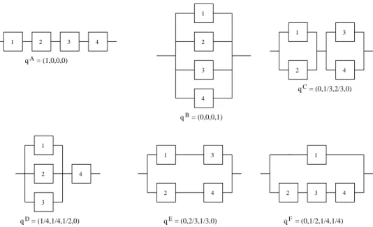
Example 1
Figure 1 presents the signatures of six coherent systems with m = 4 exchangeable com-ponents. Suppose that n = 4 components exchangeable with those in such a system were tested, leading to ordered failure timest1 < t2 < t3 < t4, which create the partitionI1, . . . , I5
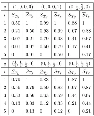
of the positive real-line. Table 1 presents the probabilities (5), denoted byjPi =P(Tj:4 ∈Ii)
for j = 1, . . . ,4 and i= 1, . . . ,5, together with the NPI lower and upper survival functions
for Tj:4 as given by (6) and (7), respectively. Table 2 presents the NPI lower and upper
survival functions ST
S(t) and STS(t) for the system failure time TS, from (8) and (9), for
each of the six systems presented in Figure 1.
Table 2 illustrates that the upper survival function for the system failure time is always equal to one in the first interval and the corresponding lower survival function is less than one. Of course, these upper and lower survival functions decrease at each observed failure time of a component in the test. The lower survival function is zero after the largest observation while the upper survival functions always remains positive. Tables 1 and 2 show that the upper survival function in intervalIi is equal to the lower survival function in interval Ii−1.
1 2 3 4 1 2 3 4 qA B q C q D q qE q = (0,0,0,1) = (1,0,0,0) 1 2 3 4 = (0,1/3,2/3,0) 1 2 3 4 = (1/4,1/4,1/2,0) 1 2 3 4 = (0,2/3,1/3,0) 1 2 3 4 = (0,1/2,1/4,1/4) F
Figure 1: Coherent systems with 4 exchangeable components
j= 1 j= 2 j= 3 j = 4 i 1Pi ST1:4 ST1:4 2Pi ST2:4 ST2:4 3Pi ST3:4 ST3:4 4Pi ST4:4 ST4:4 1 0.500 0.500 1 0.214 0.786 1 0.071 0.929 1 0.014 0.986 1 2 0.286 0.214 0.500 0.286 0.500 0.786 0.171 0.757 0.929 0.057 0.929 0.986 3 0.143 0.071 0.214 0.257 0.243 0.500 0.257 0.500 0.757 0.143 0.786 0.929 4 0.057 0.014 0.071 0.171 0.071 0.243 0.286 0.214 0.500 0.286 0.500 0.786 5 0.014 0 0.014 0.071 0 0.071 0.214 0 0.214 0.500 0 0.500
Table 1: jPi, STj:4(t) andSTj:4(t) fort ∈Ii, forn = 4 andm= 4
This is a property that generally holds for the lower and upper survival functions in this paper, and which follows directly from (6) and (7).
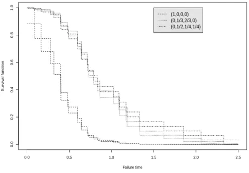
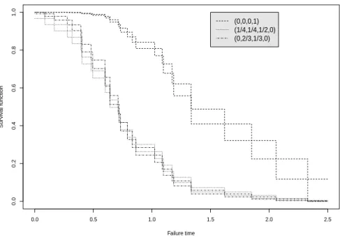
Figures 2 and 3 present the NPI lower and upper survival functions for the six systems in Figure 1 based onn = 30 observations of component failure times, simulated from the Weibull distribution with shape parameter 2 and scale parameter 1. The 30 ordered simulated component failure times are given in Table 3.
The signatures of systems C and F are not stochastically ordered, which leads to their NPI lower and upper survival functions crossing as is illustrated in Figure 2, and the same applies for systems D and E, shown in Figure 3. These lower and upper survival functions clearly indicate the differences in the system reliability for these six systems. However, one may wish to quantify the differences in reliability more precisely, a new approach that can be used for this will be presented in Section 4.
q (1,0,0,0) (0,0,0,1) (0,13,23,0) i STS STS STS STS STS STS 1 0.50 1 0.99 1 0.88 1 2 0.21 0.50 0.93 0.99 0.67 0.88 3 0.07 0.21 0.79 0.93 0.41 0.67 4 0.01 0.07 0.50 0.79 0.17 0.41 5 0 0.01 0 0.50 0 0.17 q (14,14,12,0) (0,23,13,0) (0,12,14,14) i STS STS STS STS STS STS 1 0.79 1 0.83 1 0.87 1 2 0.56 0.79 0.59 0.83 0.67 0.87 3 0.33 0.56 0.33 0.59 0.44 0.67 4 0.13 0.33 0.12 0.33 0.21 0.44 5 0 0.13 0 0.12 0 0.21 Table 2: ST S(t) and STS(t) fort ∈Ii 0.086 0.167 0.277 0.319 0.394 0.400 0.402 0.481 0.494 0.599 0.601 0.642 0.642 0.712 0.720 0.732 0.790 0.832 0.863 1.023 1.088 1.097 1.172 1.185 1.334 1.336 1.620 1.851 2.060 2.329
Table 3: 30 simulated component failure times for Example 1
Example 2
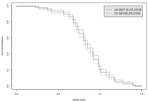
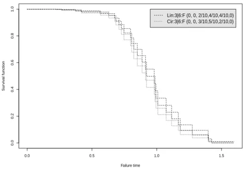
To further illustrate the NPI lower and upper survival functions for systems presented in this paper, consider linear and circular consecutive k-out-of-m:F systems, which fail if and only ifk or more linearly or circularly ordered components fail. Such systems have received much attention in the reliability literature in recent years, particularly also with focus on their signatures [10, 11, 12]. Table 4 givesn = 30 component failure times simulated from a Weibull distribution with shape parameter 3 and scale parameter 1. Figure 4 presents the NPI lower and upper survival functions, based on these data, for both a linear and circular consecutive 2-out-of-4:F system, for which the signatures are also given in the figure. The circular system fails for all neighbouring pairs of failing components for which the linear system fails, but in addition it also fails if only the first and last ordered components fail. This results in the circular system being less reliable than the linear system, as shown in Figure 4. Figure 5 presents similar NPI lower and upper survival functions for the linear and circular consecutive 3-out-of-6:F systems based on the same component failure data.
0.0 0.5 1.0 1.5 2.0 2.5 0.0 0.2 0.4 0.6 0.8 1.0 Failure time Sur viv al function (1,0,0,0) (0,1/3,2/3,0) (0,1/2,1/4,1/4)
Figure 2: The lower and upper survival functions
These systems are clearly more reliable early on than the 2-out-of-4 systems. For all these four systems considered, the lower survival function is zero beyond the largest observed component failure time, t = 1.425, reflecting that the data provide no evidence in favour of survival beyond this time, yet the corresponding upper survival functions are positive reflecting the fact that such survival cannot be deemed to be impossible on the basis of the 30 observations only.
0.223 0.265 0.372 0.419 0.564 0.630 0.675 0.685 0.709 0.727 0.747 0.798 0.807 0.824 0.850 0.887 0.914 0.921 0.981 0.987 0.994 1.008 1.073 1.115 1.167 1.182 1.275 1.397 1.400 1.425
Table 4: 30 simulated component failure times for Example 2
3
Comparing failure times of two systems
System signatures provide a straightforward way to compare the reliability of two systems with m exchangeable components (so both systems having components of the same single type) if the signatures are stochastically ordered [1]. Let the signature of system A be qa
and of systemB be qb, and let the failure times of these systems be Ta and Tb, respectively.
If Pm j=rq a j ≥ Pm j=rq b
0.0 0.5 1.0 1.5 2.0 2.5 0.0 0.2 0.4 0.6 0.8 1.0 Failure time Sur viv al function (0,0,0,1) (1/4,1/4,1/2,0) (0,2/3,1/3,0)
Figure 3: The lower and upper survival functions
a comparison is even possible if the two systems do not have the same number of compo-nents, as one can always increase the length of a system signature in a way that does not affect the corresponding system’s failure time distribution [1], hence one can always make the two systems’ signatures of the same length. However, many systems’ structures do not have corresponding signatures which are stochastically ordered. For example, the signatures (1 4, 1 4, 1 2,0) and (0, 2 3, 1
3,0) in the example in Section 2 are not stochastically ordered.
There-fore, this section presents a different way to compare the random failure times Ta and Tb
of two systems A and B within the NPI framework, namely by considering the event that system B does not fail before system A, so Ta ≤ Tb. This has the further advantage of
being applicable to any two independent systems, so systems that each only have a single type of components but with the components of system A of a different type than those of system B. Subsection 3.1 presents NPI lower and upper probabilities for the eventTa ≤Tb
for two systems that share the same type of components, followed in Subsection 3.2 by such results for two systems with different types of components. Subsection 3.3 generalizes this by considering the event Ta ≤ Tb +δ and how the NPI lower and upper probabilities for
this event behave as a function of δ. This enables a more detailed insight into the actual difference between the random lifetimes of the systems A and B.
0.0 0.5 1.0 1.5 0.0 0.2 0.4 0.6 0.8 1.0 Failure times Sur viv al functions Lin:2|4:F (0,1/2,1/2,0) Cir:2|4:F(0,2/3,1/3,0)
Figure 4: The lower and upper survival functions
3.1
Two systems with components of a single type
Consider two systems A and B withm components each and all their components assumed to be exchangeable, so both systems share components of a single type. Using the results presented in Section 2, it is easily seen that a similar result holds for the NPI lower and upper probabilities as for precise probabilities mentioned above, namely if Pm
j=rq a j ≥ Pm j=rq b j for
allr= 1, . . . , mthenP(Ta> t)≥P(Tb > t) andP(Ta > t)≥P(Tb > t) for allt >0. If the
signatures qa and qb are not stochastically ordered, a different way to compare the systems’
failure times is needed, and indeed it is natural to consider the event Ta ≤ Tb. This does not require both systems to have the same number of components, so let system A consist of ma components and system B of mb components, where the failure times of all ma+mb
components are assumed to be exchangeable. Let the ordered random failure times of the components in systemAbeTa
1:ma ≤T
a
2:ma ≤. . .≤T
a
ma:ma and let the ordered random failure
times of the components in system B be T1:bmb ≤T2:bmb ≤ . . .≤Tmbb:mb. Using the signature
qa and qb of these systems, the following equality holds [1]
P(Ta≤Tb) = ma X i=1 mb X j=1 qiaqjbP(Tia:m a ≤T b j:mb) (12)
This equality can be used directly in NPI, as the probabilities in the sum on the right-hand side of (12) are precise-valued in NPI, so no use of lower and upper probabilities is required.
0.0 0.5 1.0 1.5 0.0 0.2 0.4 0.6 0.8 1.0 Failure time Sur viv al function Lin:3|6:F (0, 0, 2/10,4/10,4/10,0) Cir:3|6:F (0, 0, 3/10,5/10,2/10,0)
Figure 5: The lower and upper survival functions
These probabilities are
P(Tia:ma ≤Tjb:m b) = ma+mb ma −1"j−1 X l=0 i−1 +l i−1 ma−i+mb−l ma−i # (13)
This follows by a straightforward counting argument, using the fact that exchangeability of the ma +mb component lifetimes includes that their orderings are all equally likely. This
implies that the ma+mb
ma
different orderings of the lifetimes of thema components in system
Aand themb components in systemB, neglecting the specific role played by each component
in the system (note that this is taken into account by the signatures), are all equally likely. For the event Ta
i:ma ≤ T
b
j:mb to occur, the number of components in system B failing before Ta
i:ma, so before the failure time of the i-th failing component in system A, can at most be j−1. For a value ofl∈ {0,1, . . . , j−1}, the corresponding term in the sum in equation (13) counts all equally likely orderings of the component failure times with precise l such times for components in system B occurring before Ta
i:ma.
Consider, for example, the systems Dand E in Figure 1, which have signatures that are not stochastically ordered. Let their failure times be denoted by Td and Te, respectively,
then this results givesP(Td≤Te) = 0.518, which can be interpreted as indicating that these two systems are about equally reliable, with system E slightly more reliable than systemD.
3.2
Two systems with different types of components
Let system A consist of ma exchangeable components, and system B of mb exchangeable
components, with the components of the different systems being of different types and their random failure times assumed to be fully independent, which means that any information about components of the type used in systemAdoes not contain any information about com-ponents of the type used in systemB. The ordered random failure times of the components in system A and of those in system B are denoted as in Subsection 3.1. Suppose that na
components exchangeable with those in system A have been tested and had ordered failure timesta
1 < ta2 < . . . < tana, and similarly that ordered observed failure times ofnb components
exchangeable with those in systemB are tb1 < tb2 < . . . < tbn
b. To avoid notational complexity
assume that there are no tied observations throughout, any tied observations can be dealt with by breaking ties by adding small values to one or more of the tied observations. Using the signaturesqa and qb of these systems, a result similar to equality (12 holds for the NPI
lower probability for the event Ta≤Tb
P(Ta≤Tb) = ma X i=1 mb X j=1 qiaqjbP(Tia:ma ≤Tjb:m b) (14) where, as presented in [9] P(Tia:ma ≤Tjb:m b) = na X l=1 Pla,i[P(Tjb:m b ≥t a l)] (15) withPla,i=P(Ta i:ma ∈(t a
l−1, tal)). The summation in (15) does not include a term forl =n+1
because P(Tb
j:mb ≥ ∞) = 0. Let vl ∈ {1, . . . , nb + 1} be such thatt
b vl−1 < t a l < tbvl, then P(Tjb:m b ≥t a l) = nb+1 X v=vl+1 P(Tjb:m b ∈(t b v−1, tbv)) (16)
The justification of (14) is similar to that of (8) in Section 2, effectively the NPI lower probabilities for the events Ta
i:ma ≤ T
b
j:mb, for i = 1, . . . , ma and j = 1, . . . , mb, can all
be attained simultaneously for the same underlying configuration of observed and future failure times for components of type A (all future observations ‘at’ the right end-point of each interval) and the same underlying configuration of observed and future failure times for components of type B (all future observations ‘at’ the left end-point of each interval) [9]. The corresponding NPI upper probability for the event Ta≤Tb is derived and justified
similarly, and is P(Ta≤Tb) = ma X i=1 mb X j=1 qiaqjbP(Tia:ma ≤Tjb:m b) (17)
where P(Tia:ma ≤Tjb:m b) = na+1 X l=1 Pla,i[P(Tjb:m b ≥t a l−1)] (18) and P(Tjb:m b ≥t a l) = nb+1 X v=vl P(Tjb:m b ∈(t b v−1, t b v)) (19) Example 3
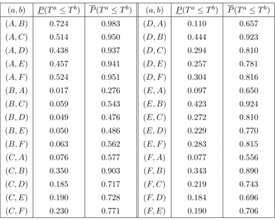
The pairwise comparison results presented in this section are illustrated using the six tems from Example 1, each with four exchangeable components but with the different sys-tems considered having different components and hence independent failure times. Table 5 presents the NPI lower and upper probabilities (14) and (17) for the events Ta ≤ Tb for
the failure times Ta and Tb for all combinations of two systems out of the six presented in Figure 1. For all these 30 events, it is assumed that na = 3 components exchangeable with
those in the system with failure time Ta and n
b = 2 components exchangeable with those
in the system with failure time Tb have been tested and that the ordering of the test data
is ta
1 < tb1 < ta2 < tb2 < ta3. Of course, the NPI lower and upper probabilities in Table 5 show
that systemA is the least reliable and system B the most reliable of these systems. Notice that the comparisons of systemsA, B, C, F with either systemDorE (whose signatures are not stochastically ordered) give very similar results, yet they all indicate that system E is slightly more reliable than systemD, the same conclusion as drawn in Subsection 3.1. This is an attractive way to compare the random failure times of two systems, which takes both the system structures and the information from the test data directly into account and considers a natural event of interest. The NPI lower probability reflects the evidence in favour of the event Ta ≤ Tb while the corresponding upper probability reflects the evidence in favour of the complementary event Ta > Tb. The difference between corresponding upper and lower probabilities, also called the ‘imprecision’, is due to the limited information available and the relatively weak modelling assumptions. In Table 5 the imprecision of most events is large, which is due to there being only 5 observations in total. If more test data are available, the imprecision typically become smaller, with the difference disappearing in the limit if the number of test data in both groups goes to infinity.
Table 6 presents the NPI lower and upper probabilities for the pairwise comparison of systems D and E, considering the event TD ≤ TE with n
D = 3 observed failure times
for components exchangeable with those in system D and nE = 2 observed failure times
for components exchangeable with those in system E, and all possible orderings of these observed failure times. These lower and upper probabilities vary of course for the different
(a, b) P(Ta≤Tb) P(Ta≤Tb) (a, b) P(Ta≤Tb) P(Ta≤Tb) (A, B) 0.724 0.983 (D, A) 0.110 0.657 (A, C) 0.514 0.950 (D, B) 0.444 0.923 (A, D) 0.438 0.937 (D, C) 0.294 0.810 (A, E) 0.457 0.941 (D, E) 0.257 0.781 (A, F) 0.524 0.951 (D, F) 0.304 0.816 (B, A) 0.017 0.276 (E, A) 0.097 0.650 (B, C) 0.059 0.543 (E, B) 0.423 0.924 (B, D) 0.049 0.476 (E, C) 0.272 0.810 (B, E) 0.050 0.486 (E, D) 0.229 0.770 (B, F) 0.063 0.562 (E, F) 0.283 0.815 (C, A) 0.076 0.577 (F, A) 0.077 0.556 (C, B) 0.350 0.903 (F, B) 0.343 0.890 (C, D) 0.185 0.717 (F, C) 0.219 0.743 (C, E) 0.190 0.728 (F, D) 0.184 0.696 (C, F) 0.230 0.771 (F, E) 0.190 0.706
Table 5: Pairwise comparisons of six systems from Figure 1
data orderings, and also the imprecision varies. If the three tested components of typeD all failed before the two of typeE, the data do not contain any evidence against the possibility that components of typeDwill always fail before components of typeE, which is reflected in
P(TD ≤ TE) = 1 in this case. Similarly, the other extreme data ordering does not provide
any evidence in favour of the possibility that components of type D will ever fail before components of type E, as reflected by P(TD ≤TE) = 0 for the final ordering in Table 6.
3.3
The difference between the failure times of two systems
The method presented in Subsection 3.2 compares the random failure times of two systems by considering the event that one fails before the other, but it does not provide insight into the actual difference between these failure times. Therefore, the approach of Subsection 3.2, using the same setting of two systems with different types of components, is now generalized by considering the event Ta ≤ Tb +δ, so Ta −Tb ≥ δ, for all real-valued δ. Of course,
the setting of Subsection 3.1 can be similarly generalized. The following generalization of equation (12), P(Ta≤Tb+δ) = ma X i=1 mb X j=1 qiaqjbP(Tia:m a ≤T b j:mb +δ)
Data ordering P(TD ≤TE) P(TD ≤TE) td1 < td2 < t3d< te1 < te2 0.548 1 td1 < td2 < t1e < td3 < te2 0.442 0.940 td1 < td2 < t1e < te2 < td3 0.371 0.869 td1 < te1 < t2d< td3 < te2 0.328 0.852 td 1 < te1 < td2 < te2 < td3 0.257 0.781 te1 < td1 < t2d< td3 < te2 0.219 0.757 te 1 < td1 < td2 < te2 < td3 0.149 0.686 td1 < te1 < t2e < td2 < td3 0.181 0.675 te1 < td1 < t2e < td2 < td3 0.072 0.580 te1 < te2 < t1d< td2 < td3 0 0.466
Table 6: Pairwise comparisons of systemsD and E with nD = 3 and nE = 2
is proven in the same way as equation (12) [1], and is intuitively logical because adding the constant value δ to the random lifetime of a system can be thought of as adding it to the lifetimes of all its components, doing so will not change the signature of the system. This immediately carries through to the NPI lower probability for this event, which is
P(Ta≤Tb+δ) = ma X i=1 mb X j=1 qiaqjbP(Tia:ma ≤Tjb:mb +δ) (20)
with the NPI lower probabilities in the sum on the right-hand side equal to
P(Tia:m a ≤T b j:mb +δ) = na X l=1 Pla,i[P(Tjb:m b +δ ≥t a l)] (21)
Letvl,δ ∈ {1, . . . , nb + 1} be such thattbvl,δ−1 < t
a l −δ < t b vl,δ, then P(Tjb:m b+δ≥t a l) = nb+1 X v=vl,δ+1 P(Tjb:m b ∈(t b v−1, tbv)) (22)
The corresponding NPI upper probability for the eventTa ≤Tb+δ is
P(Ta≤Tb+δ) = ma X i=1 mb X j=1 qiaqjbP(Tia:ma ≤Tjb:m b +δ) (23) where P(Tia:ma ≤Tjb:m b+δ) = na+1 X l=1 Pla,i[P(Tjb:m b +δ ≥t a l−1)] (24) and P(Tjb:m b+δ≥t a l−1) = nb+1 X v=vl,δ P(Tjb:m b ∈(t b v−1, tbv)) (25)
Compared to the NPI lower and upper probabilities presented in Subsection 3.2, which correspond to those for δ = 0 here, calculation of these NPI lower and upper probabilities just follows from shifting the mb test observations for components exchangeable to those
in system B by adding δ, or alternatively by subtracting δ from each observation ta l. For
changing value ofδ, these NPI lower and upper probabilities only change ifδ is large enough to change the ordering of the tb
1, . . . , tbnb relative to the values t
a
1 −δ, . . . , tana −δ, such a
change of the ordering can happen for at most na × nb different values of δ. Therefore,
P(Ta ≤Tb+δ) and P(Ta ≤Tb+δ) can have at mostna×nb+ 1 different values (including
the case δ = 0), and as function of δ these lower and upper probabilities are step functions which change value at the same na×nb points, making their computation straightforward
unless na×nb is very large.
Example 4
SystemsD and E of Figure 1 have been of interest as their signatures are not stochastically ordered. Assume now that they have different types of components, with nd = ne = 30
components exchangeable with those of each type in the respective system having been tested, leading to the failure times in Table 7. The ordered failure times are given in Table 6, which for system D were simulated from a Weibull distribution with shape parameter 3 and scale parameter 1, and for systemE from a Weibull distribution with shape parameter 2 and scale parameter 1.
System D System E 0.223 0.747 0.994 0.154 0.585 1.076 0.265 0.798 1.008 0.155 0.598 1.169 0.372 0.807 1.073 0.347 0.642 1.239 0.419 0.824 1.115 0.402 0.692 1.248 0.564 0.850 1.167 0.483 0.738 1.327 0.630 0.887 1.182 0.512 0.822 1.421 0.675 0.914 1.275 0.513 0.843 1.569 0.685 0.921 1.397 0.548 0.848 1.643 0.709 0.981 1.400 0.563 0.863 1.735 0.727 0.987 1.425 0.574 0.938 2.565
Table 7: Simulated ordered component failure times for Example 4
Figure 6 presents the NPI lower and upper probabilities for the event Td ≤ Te +δ as functions of δ. In the top-left figure, Figure 6.1, these functions are given for the data in Table 7. For these data, these functions remain constant for values of δ less than −2.342
or greater than 1.271, as in these cases the two data sets are completely non-overlapping, which shows in the fact that the NPI lower probability for this event is equal to zero for
δ < −2.342 and the NPI upper probability for this event is equal to one for δ > 1.271.
Actually, the changes in these NPI lower and upper probabilities at δ equal to −2.342 or 1.271 are very small and not well visible in Figure 6.1. The same is true at other values of
δ close to these minimal and maximal ones at which the NPI lower and upper probabilities change. At δ=−2.342, the NPI lower probability Td≤ Te+δ increases from 0 to 0.00013 and the NPI upper probability increases from 0.03630 to 0.03656, while at δ = 1.271 the lower probability increases from 0.9870 to 0.9872 and the upper probability increases from 0.99996 to 1.
The 3 further figures included in Figure 6 show the effect of substantial changes to the actual observations, that is changes that actually change the order of the observations, and hence how the NPI lower and upper probabilities for the eventTd ≤Te+δ adapt to changes in the component test data. First, the largest observed failure time for system D, 1.425, is replaced by 3.425, which makes it the largest observed value in both sets of data. The resulting NPI lower and upper probabilities for the event Td ≤ Te +δ as functions of δ
are presented in Figure 6.2, but the effect on the figures is not well visible when compared to the original situation in Figure 6.1. Figures 6.3 and 6.4 show the NPI lower and upper probabilities with the largest 4 and 10, respectively, values for System D, as given in Table 7, changed by adding 2 to the original data values, which implies that these all become larger than the largest observation for System E. Now the effect is clear in both figures, and of course substantially stronger in case 10 observations have been changed. Figure 7 presents the same functions of Figures 6.1 and 6.4, so for the original data and with 10 values changed, on a larger scale to see the differences more clearly. While the differences for the larger values ofδare obvious, this figure shows that there have also been some small changes for δ close to 0 and even for negative values of δ.
4
Concluding remarks
This paper has introduced the use of signatures in the study of system reliability with lower and upper probabilities. There are many related research challenges, for example a slightly more challenging topic is simultaneous comparison of more than two systems’ failure times. The NPI lower and upper probabilities for pairwise comparisons, as presented in Section 3, cannot be combined directly into such quantifications for multiple comparisons. For example, it may be of interest to consider the event that a particular one of the systems considered is the most reliable in the sense of its random failure time being the largest of all systems’
−4 −2 0 2 4 0.0 0.4 0.8
1
−4 −2 0 2 4 0.0 0.4 0.82
−4 −2 0 2 4 0.0 0.4 0.83
−4 −2 0 2 4 0.0 0.4 0.84
Figure 6: The difference of failure times of two systems
failure times, so it is of interest to generalize the method presented in Section 3 to derive NPI lower and upper probabilities for such events. This can be done in NPI along the lines of such multiple comparisons as presented in [13].
Substantially more challenging research topics include generalization of the approach presented in this paper for test data including right-censored observations, as often occur for failure time data [14]. This first requires development of NPI for future order statistics with such data, which is a challenge indeed as equation (4) cannot be applied in such a setting and simple counting arguments may need to be replaced by complex optimisation methods. Once the approach has been extended to include right-censored data, multiple comparisons are also of interest and can follow the same approach as presented in [15, 16].
Signatures can also be used for reliability quantification for systems for which only failure or non-failure upon request for functioning is of interest, so without explicit focus on failure time. Applying this to systems with exchangeable components will be relatively straightfor-ward and will generalize the results in [17]. In that paper a conjecture was formulated about optimal redundancy allocation, in line with the results in [18] and [19] for different systems;
−4 −2 0 2 4 0.0 0.2 0.4 0.6 0.8 1.0
Figure 7: The difference of failure times of two systems
analysis based on signatures might facilitate the proof of that conjecture.
There are major research challenges to the general theory of signatures, solutions to which may be of particular interest when working with lower and upper probabilities. For example, the fact that the theory of signatures [1] only applies to systems with exchangeable components is a very considerable restriction on the practical relevance of signatures and the related methods for reliability quantification. While there is clearly no direct generalization of signatures to systems with multiple types of components, the basic idea to separate aspects of the system structure and of specific component lifetime distributions to support quantification of reliability could possibly also lead to methods that would simplify such quantification when theory of lower and upper probabilities is used. A further challenge is in deriving system signatures for more substantial systems, where it may be of interest to consider approximation of system signatures. It may be possible to develop a theory of ‘imprecise signatures’, so sets of signatures that are based on partial information about the system considered. There are other statistical approaches that use lower and upper probabilities to quantify uncertainty [4], combination of such approaches with signatures
also provides many opportunities and challenges for research. This paper opens up a wide area of interesting research topics, progress on which will help development and application of NPI methods for system reliability.
Acknowledgements
We thank two referees for their supportive comments and suggestions for improving the presentation of this paper.
References
[1] Samaniego F.J. (2007).System Signatures and their Applications in Engineering Relia-bility. Springer.
[2] De Finetti B. (1974). Theory of Probability. Wiley.
[3] Barlow, R.E., Proschan, F. (1975). Statistical Theory of Reliability and Life Testing: Probability Models. Holt, Rinehart and Winston.
[4] Utkin L.V., Coolen F.P.A. (2007). Imprecise reliability: an introductory overview. In:
Computational Intelligence in Reliability Engineering, Volume 2: New Metaheuristics, Neural and Fuzzy Techniques in Reliability, G. Levitin (Ed). Springer, pp. 261-306.
[5] Augustin T., Coolen F.P.A. (2004). Nonparametric predictive inference and interval probability. Journal of Statistical Planning and Inference 124 251-272.
[6] Coolen F.P.A. (2006). On nonparametric predictive inference and objective Bayesianism.
Journal of Logic, Language and Information 15 21-47.
[7] Walley P. (1991). Statistical Reasoning with Imprecise Probabilities. Chapman & Hall.
[8] Weichselberger K. (2001). Elementare Grundbegriffe einer Allgemeineren Wahrschein-lichkeitsrechnung I. Intervallwahrscheinlichkeit als Umfassendes Konzept. Physika.
[9] Coolen F.P.A., Maturi T.A. (2010). Nonparametric predictive inference for order statis-tics of future observations. In: Combining Soft Computing and Statistical Methods in Data Analysis, C. Borgelt et al(Eds). Springer, pp. 97-104.
[10] Eryilmaz S. (2010). Review of recent advances in reliability of consecutive k-out-of-n
[11] Navarro J., Eryilmaz S. (2007). Mean residual lifetimes of consecutive-k-out-of-n sys-tems. Journal of Applied Probability44 82-98.
[12] Eryilmaz S. (2011). Circular consecutive k-out-of-n systems with exchangeable depen-dent components. Journal of Statistical Planning and Inference 141 725-733.
[13] Coolen F.P.A., van der Laan P. (2001). Imprecise predictive selection based on low structure assumptions. Journal of Statistical Planning and Inference98 259-277.
[14] Coolen F.P.A., Yan K.J. (2004). Nonparametric predictive inference with right-censored data. Journal of Statistical Planning and Inference126 25-54.
[15] Coolen-Maturi T., Coolen-Schrijner P., Coolen F.P.A. (2011). Nonparametric predictive selection with early termination of experiments. Journal of Statistical Planning and Inference141 14031421.
[16] Coolen-Maturi T., Coolen-Schrijner P., Coolen, F.P.A. (2011). Nonparametric predic-tive multiple comparisons of lifetime data. Communications in Statistics - Theory and Methods, to appear.
[17] Coolen F.P.A., Aboalkhair A.M., MacPhee, I.M. (2009). Nonparametric predictive sys-tem reliability with all subsyssys-tems consisting of one type of component. In: Risk and Decision Analysis in Maintenance Optimization and Flood Management, M.J. Kallen, S.P. Kuniewski (Eds). IOS Press, pp. 85-98.
[18] Coolen-Schrijner P., Coolen F.P.A., MacPhee I.M. (2008). Nonparametric predictive in-ference for system reliability with redundancy allocation.Journal of Risk and Reliability
222 463-476.
[19] MacPhee I.M., Coolen F.P.A., Aboalkhair A.M. (2009). Nonparametric predictive sys-tem reliability with redundancy allocation following component testing.Journal of Risk and Reliability223 181-188.