Learning Embeddings for Graphs and Other High Dimensional Data

(1)

Hasti Narimanzadeh

School of Science

Thesis submitted for examination for the degree of Master of Science in Technology.

Espoo 31.12.2019

Thesis supervisor and advisor:

(2)

Author: Hasti Narimanzadeh

Title: Learning Embeddings for Graphs and Other High Dimensional Data Date: 31.12.2019 Language: English Number of pages: 5+54 Computer Science

Professorship: Theoretical Computer Science

Supervisor and advisor: Prof. Parinya Chalermsook

An immense amount of data is nowadays produced on a daily basis and extracting knowledge from such data proves fruitful for many scientific purposes. Machine learning algorithms are means to such end and have morphed from a nascent research field to omnipresent algorithms running in the background of many applications we use on a daily basis. Low-dimensionality of data, however, is highly conducive to efficient machine learning methods. However, real-world data is seldom low-dimensional; on the contrary, real-world data can be starkly high-dimensional. Such high-dimensional data is exemplified by graph-structured data, such as biological networks of protein-protein interaction, social networks, etc., on which machine learning techniques in their traditional form cannot easily be applied.

The focus of this report is thus to explore algorithms whose aim is to generate representation vectors that best encode structural information of the vertices of graphs. The vectors can be in turn passed onto down-stream machine learning algorithms to classify nodes or predict links among them. This study is firstly prefaced by introducing dimensionality reduction techniques for data residing in geometric spaces, followed by two techniques for embedding vertices of graphs into low-dimensional spaces.

Keywords: Graph embeddings, Network embedding, Machine learning, dimen-sionality reduction algorithms, random walks, spectral techniques

(3)

Preface

Like most things, I would like to keep this preface minimal. So, first and foremost, I would like to thank my supervisor and advisor Parinya Chalermsook for his support throughout, and for granting me the autonomy to do research on my topic of interest. As I recall, he once told me nothing repels him more than unmotivated students; I hope I haven’t let him down in that respect.

The friendships made, I will treasure always. So big thanks to Wanchote, Sor-rachai, Amit, Ly, and Nidia.

My best friends and partners in crime, Armin and Mona, who also happen to be my brother and sister, I am indebted to you for your guidance and support.

The process would have been a lot more difficult if it wasn’t for both emotional and intellectual support, as well as the late night dinners and orange juices Arash provided every single day. Arash, you simply make life better, thank you.

This wouldn’t be possible after all without my parents giving me the gift of life. Nader and Shahrbanou, thank you for every step of the way. I will be beholden to you always.

Otaniemi, 31.12.2019

(4)

1 Introduction And Outline Of The Thesis

Machine Learning (ML) embodies the conversion of experience to knowledge in the realm of computers. The term originates from computers programmed to “learn” from the input data available to them. Machine learning is where the sheer abundance of digital data intersects with mathematical frameworks. In loose terms, the input to such a learning model is the training data and the output is some expertise.

Such pattern recognition in data has a long history: The astronomical observations of Tycho Brahe in the 16th century allowed Kepler to discover the empirical laws of planetary motion, which in turn paved the way for developments in classical mechanics [1]. And nowadays its applications are innumerable, ranging from recommendation systems to image classification. Moreover, the type of data used in such models runs the gamut: images, words, numbers, clicks on social media, etc., enabling all the more applications to be born.

The nature of the input data can speak to a machine learning model’s efficacy. Conventionally, data used by learning algorithms are represented in Euclidean space. However, in many real-world scenarios, the data are represented as graphs with complex relationships between its entities. Examples of such data are social networks or biological protein-protein networks [2]. Attempts to apply machine learning algorithms established the area of representation learning on graphs whose goal is to encode graphs in low-dimensional embeddings such that the graph structure and properties are maximally preserved. The encoded graph-structured data can be in turn fed into a downstream machine learning algorithm as feature inputs.

Traditionally, representation vectors were hand-crafted for graphs, discarding the graph properties encoded in the graph structure. With the advancement of machine learning paradigms, research gravitated towards applying machine learning algorithms on graphs. Fast forward to now, techniques in representation learning on graphs, also referred to as graph embedding, are broadly categorized into three categories of factorization based, random walk based, and deep learning approaches. These categories include countless algorithms and there is ongoing research to concoct all the more with more efficiency, as well as construct a consistent theoretical foundation for all techniques.

In Section2we explore the mathematical bedrock of machine learning algorithms and subsequently study a well-known dimensionality reduction technique on data in geometric spaces and how it bears resemblance to a factorization based graph embedding algorithm we study in Section 4. In Section 3 we review the general idea of graph embeddings and provide a literature review of some existing techniques. In Section5, a random walk embedding technique is explored, and lastly some challenges that lie ahead are discussed.

(7)

2 Machine Learning

We begin to study how learning is mathematically defined in the context of machine learning. In so doing, we lay groundwork and justification for numerous elements of the subsequent algorithms and concepts. It can also be viewed as an attempt to bring the two areas of graph embeddings and machine learning closer.

2.1 Notation

The following notations are used throughout this manuscript:

A scalar is denoted by a roman (non-bold) lowercase letter, e.g.b ∈R. We denote vectors in Rd _{by bold lowercase letters, e.g.} _x_{= (}_x

1, x2, . . . , xd)T is a column vector whose elements are x1, x2, . . . , xd (denoted by roman, indexed lowercase letter) and where T _{denotes the transpose operator. Norm function} _k_x_k _{without any indices} refers to L2-norm: kxk=kxk₂ = s X i x2 i

A bold uppercase letter signifies a matrix, for example M ∈ Rd×d _{is a square} matrix of dimensionsdbyd. Elements of matrixMare denoted using roman, capital, double-indexed letters such asMij

BothPandP rmay donate the probability of a random variable. The dot product of two vectors is indicated by a dot character, e.g.w.x is the dot product of vectors w and x.

2.2 A Formal Mathematical Learning Model

Learning has a concrete mathematical notion that is essential to understanding how learning algorithms operate. To this end, we attempt to present an all-encompassing albeit terse description of a formal model that describes a simple learning scenario. Shalev-Shwartz and Ben-David [3] offer a simple but powerful example of a learning problem which we can deliberately examine to seek the primary components of a learner. Suppose we have a few papayas at our disposal and would like to determine their tastiness. Drawing on prior experience we decide to use two features of papayas to assess tastiness: their color and softness. We begin tasting papayas, noting their tastiness, color, and softness. Ultimately, we would have a sample of tasted papayas, having recorded their two features of softness and color. We then arrive at a prediction rule for predicting the tastiness of future papayas.

We begin with the fundamental mathematical components of the said learning problem.

• Learner’s input: Learner is given the following in a basic statistical setting: – Domain set: Often denoted by X, it is the set of objects under study that we wish to label. In the above-mentioned learning task, the domain

(8)

set is all the papayas. Each object of the domain set is often referred to as data points or instances and is usually represented as a vector of features or dimensions.

– Label set: This is a set, often denoted byY, including all the labels we wish to assign to each data point in the domain set. For our example, the label set is thus tasty and not tasty which we can mathematically formulate as either {−1,+1} or{1,0}. In this specific type of learning scheme, we have the “correct” label for each papaya in the domain set. Nonetheless, this may not always be the case. In fact, learning tasks to which labels are not available are dubbed unsupervised learning; whereas learning schemes that exploit existing correct labels to tune their parameters are named supervised learning. The most notable example of the former is clustering [4]. And the papaya example is an instance of supervised learning, more specifically, a classification task.

X and Y coupled together form a set, namely the training data set S =

{(x1, y1), . . . ,(xN, yN)}, where yi is the correct label corresponding to data point xi. Usually, the domain and label sets are fed to learner as the this training data set.

• Learner’s output: The learner is expected to learn a prediction rule, or better yet a mapping from the domain set to the label set h :X −→ Y, which also constitutes the output of the learner. The mapping is also called thehypothesis or the predictor. The hypothesis is the rule that the learner adopts to assess the tastiness of future papayas based on their color and softness. The correct labelyi is however generated by a functionf, that isf(xi), wheref :X −→ Y. The “correct” labelling function f is what the learner tries to emulate to the best of its abilities.

• The probability distribution of the dataThe training data set is sampled from an arbitrary probability distribution. In our current learning scheme, we assume the learner does not have any knowledge of the underlying distribution

Dand does not try to estimate it. We will encounter a specific type of learning paradigm in Section 2.5, that the estimation of the underlying probability distribution of the generated data lies at the heart of the learning task. This is however not the case here.

• Measure of performance The efficacy of the trained learner is determined by how the learner performs on a random, or rather unseen data point drawn from the underlying distribution. In that sense, thetrue error of the hypothesis

h is defined to be the probability of label of a random data point—drawn from probability distribution D—not being equal to the correct label. More precisely,

(9)

This measure determines thegeneralization power of the learning algorithm and for this reason it is also called thegeneralization error of the learner. The two terms, “generalization error” and the “true error ” may be used interchangeably throughout.

The generalization error is measured with respect to the underlying distribution

D and the correct labelling function f, hence the subscript (D, f). However, the learner has no knowledge of the two and therefore is incapable of directly calculating the true error. This lack of knowledge about the target function and the distribution of the data underpins the necessity of a different notion of error which the hypothesis h can compute. This brings us to the following learning paradigm: Empirical Risk Minimization.

2.3 Empirical Risk Minimization

The learner only has access to the training data set drawn from an unknown distri-bution. It attempts to learn a hypothesis h:X −→ Y that approximates a target functionf that has generated the labels of the training samples. Since the learner has no knowledge of either f or D and has the training data set at its disposal, it computes the training error it incurs on the training samples. In the simplest of forms, such as the papaya example we’ve discussed so far, this error can be calculated as follows.

LS(h) = |{i∈[N] :h(xi)6=f(xi)}|

N (2)

The subscript emphasizes the dependence of the hypothesis loss on the training data set. And due to this dependence, it is also called empirical risk or empirical error. Intuitively, the hypothesis attempts to do well on the training data set, or rather, minimize the empirical risk and for this reason, this learning paradigm is namedEmpirical Risk Minimization or ERM for short.

2.3.1 Empirical Risk Minimization and Overfitting

Albeit ERM seems intuitive, Shalev-Shwartz and Ben-David [3] outline how it can lead tooverfitting. Overfitting is the phenomenon that the hypothesis h performs well on the training data set while performing poorly on the unseen data, concluding that the generalization error is too high for such a hypothesis. A common solution to this overfitting problem is to constrict the search space. Strictly speaking, the learner chooses a set of predictors, namely the hypothesis class denoted by H, before seeing the training data set. Thereafter the problem amounts to finding a mapping function

h∈ H that performs well enough on the training data set. Therefore, formally, we would like to find the set of hypotheses in H that achieve the minimum empirical error

ERMH(S)∈arg min h∈H

(10)

The choice of the hypothesis class is thus based on some prior knowledge about the task at hand and leads to a fundamental question in learning theory of how to choose the hypothesis class H to ensure ERMH learning will not overfit. One solution to preventing overfitting is restricting the hypothesis class by imposing an upper bound on its size—which is the number of hypotheses in the hypothesis class. Theorem (1) states that ERM will not overfit provided the hypothesis space H is finite and the training sample is sufficiently large.

Theorem (1) makes two simplifying assumptions: the i.i.d. Assumption and the realizability Assumption. The i.i.d. assumption, on which numerous machine learning algorithms are founded, states that data points in the training data set are independently and identically distributed. The realizability assumption is that there exists h∗ ∈ H such that LD,f(h∗) = 0. Meaning that for a random data point x sampled fromD, the true label given byf(x) equals the calculated labelh∗(x) with probability 1. Therefore, Theorem (1) must show that

LD(hS)< with probability at least 1−δ for accuracy parameter >0 and confidence parameter 1−δ.

That is, the true error of the hypothesis chosen by the ERM is sufficiently low, that is LD(h)< . The confidence parameter is to cater for cases that we may draw “unrepresentative” samples from the underlying distribution.

Theorem 1 (FINITE theorem) Let H be a finite hypothesis space and assume realizability. Let and δ∈(0,1) be the accuracy and the confidence respectively. And consider the sample size N to be

N ≥ log (|H|/δ)

Let the Empirical Risk Minimization algorithm select the hypothesishs over the sample S ∼ DN_{. Then}

LD(hs)≤ with probability at least 1−δ

Proof: Define H = {h ∈ H: LD(h) > }, which includes all hypotheses with error more than > 0. We then move on to calculate the probability that any hypothesis in H is consistent with a sampleS of size N

(11)

P[∃h∈ H: LS(h) = 0]

=P[LS(h1) = 0∨. . .∨ LS(h|H|) = 0]

≤ X

h∈H

P[LS(h) = 0], (Union bound) Given we have defined the error of the hypotheses to be

LD(h) = Px∼D[h(x)6=f(x)]> we have Px∼D[h(x) =f(x)]<1− therefore ≤(1−)N|H| ≤(1−)N|H|

Hence, the probability that all the hypotheses that are consistent with sample S

have error at most is at least 1−(1−)N|H|. We would like to select N such that (1−)N|H| ≤δ This yields N ≥ ln( 1 δ) + ln|H| −ln (1−) ≥ ln (|H|/δ)

Therefore, in most machine learning scenarios, a suitableloss function, also known as thecost function, is defined based on the task at hand and subsequently optimized (minimized) by an optimization method of choice. The choice of the loss function primarily hinges on the types of parameters we would like to predict and also affects the choice of the optimization method.

2.4 The Perceptron Algorithm: A Linear Classifier

We study a simple yet powerful linear classifier, the Perceptron [5], to see how the components of a learning task we set forth earlier play out. We consider a binary classification task, i.e. Y = {−1,+1} and a training data set X = {x1, . . . ,xN} where xi ∈Rd for all i.

For such a training set, we would like to find a linear classifier, that is a hyper-plane, which correctly classifies all the data points. A hyper-plane is characterized by the normal vector which is perpendicular to the hyper-plane w∈Rd _{and a} _bias parameter b∈R. Thus, the learning task amounts to finding the most suited normal vector and bias. Let the potential hyper-planes, i.e. linear predictors, be the following set of functions

(12)

For any data point xthere are two options—minus the case where the data point resides on the hyper-plane and thus the dot product of the two equals zero—: the data point can form an acute angle with the normal vector and thus the functions in

Ld would output a positive number. Or the data point forms an obtuse angle with the normal vector in which case the output would be negative. In any case it is not hard to see that for the predictor to classify data point xi with the corresponding

correct label yi correctly, the following must hold true yi(w.xi+b)≥0

In order for the predictor to return a valid −1 or +1 label upon receiving a data point x, we apply the sign function to predictors, that is

sign(w.x+b) =    +1, if w.x+b ≥0. −1, otherwise. (3)

This brings us to the hypothesis class designed for binary classification tasks, namely the class ofhalfspaces

HSd= sign◦Ld={x7→sign(hw,b(x)) :hw,b∈Ld} where

hw,b(x) =w.x+b

The Perceptron is an iterative algorithm that finds a linear predictor in such hypothesis class for a given training data set, using the following loss function upon receiving a data point xi and its corresponding correct label yi ∈ {−1,+1}

`(xi,yi)(w, b)) =    0, if yi(w.xi+b)≥0. −yi(w.xi+b), otherwise. (4) The total loss function is the summation of the loss incurred on all the data points in the training data set S ={x1, . . . ,xN}

LS(hw,b) = N

X

i

`(xi,yi)(hw,b)

Intuitively, if the predictor classifies the data point correctly, no error should be incurred. However, if not, the learner should be penalized in proportion to how wrong it was. The convexity of such a loss function guarantees a global optimum, which is the holy grail of any machine learning algorithm.

To optimize the above loss function, Perceptron utilizesstochastic gradient descent (SGD). Stochastic gradient descent is a variation of gradient descent (GD). Both algorithms are unconstrained optimization techniques that aim to minimize a function by iteratively nudging the parameters from their initial values in the opposite direction of the gradient of the loss function, until they converge. The two techniques differ in how they treat the training data set. Gradient descent makes a pass throughall the

(13)

data points for each update of the parameters, whereas stochastic gradient descent performs an update of parameters based on every single single data point.

Implementation of stochastic gradient descent is outlined in Algorithm 1. Algorithm 1: SGD(η, T,S) for minimizing f(w)

Input: step sizeη

number of iterations T

labeled training data set S

Output: function parameters w Initialize w(1) ₌₀

for t= 1, . . . , T do

Draw (x, y)∈ S randomly w(t+1)₌_w(t)₋_η_∇_`_(w(t)_{; (x}_{, y}₎₎

return w(T+1)_;

Parameters η and T ensure the convergence of SGD [3, 1].

The Perceptron uses SGD (with step size η= 1) to minimize the loss function defined in Equation (4) (as can be seen by the partial derivatives with respect to the weights and bias used in the update steps) and is described in Algorithm2. Novikoff [6] proves that the Perceptron converges if the data is linearly separable (there exists a linear classifier that classifies all the data points in the training data set correctly). The theorem is stated below in Theorem 2. It is interesting how neither the size of domain setX nor the dimensionality of the data points affect the bound on number of mistakes the perceptron makes. The Perceptron does not necessarily converge for non-linearly separable data [3].

Theorem 2 (Novikoff, 1962) Consider data pointsx1, . . . ,xN ∈Rdwhere||xi|| ≤ r for all i ∈[N] for some r > 0. We assume there exists ρ >0 and w∗ ∈ Rd _such that ρ≤ yi(w∗.x)

||w∗_|| (linear separability) for all i∈[N]. Then, we can state the following

about the number of perceptron updates (i.e. the number of prediction mistakes) T

when processing x1, . . . ,xN is

T ≤ r 2

ρ2

The Perceptron is one of a plethora of classifiers, linear or otherwise, in the machine learning realm. It is, however, one of the most simple classification algorithms that also lays the groundwork for a more competent set of classifiers known as the support vector machines [3, 1]. The Perceptron is also a precursor to a different learning paradigm known as artificial neural networks, that will be briefly discussed in Subsection2.6.

2.5 Generative Models

When following a discriminative approach, such as the Perceptron algorithm in Section 2.4, we are oblivious to the underlying distribution of the data. In other

(14)

Algorithm 2: perceptron(S, T) Input: labeled training data setS

number of iterations T

Output: predictor parameters w, b

Initialize w=0 and b = 0 for t= 1, . . . , T do if ∃i s.t. yi(w(t).xi+b(t))<0then w(t+1) ₌_w(t)₊_y ixi b(t+1) =b(t)+yi else return w(T+1), b(T+1);

(15)

words, we do not make any assumptions about the underlying distribution of which the observed data are sampled from and do not attempt to learn it, rather we learn a predictor. However, in generative models, we assume the data points are drawn from a specific parametric distribution whose parameters we attempt to estimate.

More specifically, the distribution of the data, the model, has a set of parameters

θ which the goal is to learn having observed data set S. In other words, we assume adistribution family for the observed data and subsequently estimate its parameters. As an example, if we assume the data is sampled from a Gaussian distribution, the parameters are the mean and the covariance,θ ={µ,Σ}. Generally, given the training data set S, we have some prior belief about θ, and the Bayes’s rule will update it in light of newly observed data

P[θ|S] = P[S|θ]P[θ]

P[S] (5)

The term P[S|θ] is the likelihood of the observed data given θ and can be viewed as a function of θ. P[θ] is called the prior, and P[S] the marginal likelihood or the evidence.

A brief description of a well-known statistical method is underway, for estimating the parameters of the distribution over the data, that is the maximum likelihood principle. Maximum likelihood aims to maximize the likelihood of the observed data which is, in turn, a function of θ, hence the name. Moreover, we will observe how maximum likelihood is similar to and differs from the empirical risk minimization (ERM) studied previously.

2.5.1 Maximum Likelihood Estimator

Simply put, maximum likelihood estimator finds the parameters of the underlying distribution for which the observed data has the highest probability. More concretely, it maximizes the likelihood function described above. Shalev-Shwartz and Ben-David [3] present a concrete example to grasp the idea of this estimator as follows:

Assume a pharmaceutical company has developed a new medicine as a cure to a deadly disease and would like to gauge the probability of patients’ survival having used the medicine. The company samples N people independently and provides them with the medicine. The sample set is denoted by S = {x1, . . . , xN}, where xi = 1 if patient i survived and xi = 0 otherwise. It can be seen that the random variable xi follows a Bernoulli distribution which can be modeled with a single parameter θ∈[0,1], indicating the probability of survival.

The goal is now to estimate θ based on the training data set S. The joint probability distribution over i.i.d. random variables is

P[xi, . . . , xN|θ] = N

Y

i=1

P[xi|θ]

(16)

P[D={xi, . . . , xN}] = N

Y

i=1

θxi₍₁₋_θ₎1−xi ₌_θP_ixi₍₁₋_θ₎P_i(1−xi) ₍₆₎

It is often more convenient to work with the logarithm of the likelihood function. Since logarithm is a monotonic function, the maxima of the logarithm of the likelihood function, log-likelihood for short, will coincide with that of the likelihood function. LetL(S;θ) denote the log-likelihood of S givenθ, which is

L(S;θ) = log(P[S ={x1, . . . , xN}]) = log(θ) X i xi+ log(1−θ) X i (1−xi)

The maximum likelihood estimation is then the parameter ˆθsuch that it maximizes the log-likelihood above

ˆ

θ ∈arg max θ

L(S;θ) (7) To find ˆθ that maximizes the log-likelihood, we take the derivative of L(D;θ) with respect to θ and set it to zero

d

dθL(S;θ) = 0

Taking the derivative of the log-likelihood of our problem, we can arrive at

P ixi θ − P i(1−xi) 1−θ = 0

Solving this equation we calculate the estimated parameter ˆθ to be

ˆ

θ =

PN

i=1xi N

The estimated probability of survival, based on maximum likelihood estimation, is just the fraction of people on the drug who have survived to the total number of the users of the drug, which also happens to be in line with our intuition as to what our best guess as to the probability of survival based on currently known data would be.

In the above-mentioned example the Bernoulli random variable was discrete. A slight modification is in order for continuous random variables. Due to the fact that for a continuous random variable X we have P[X= x] = 0, we define the log-likelihood to be the log of theprobability density function of X atx. More specifically, given an i.i.d. training data set S ={x1, . . . , xN} sampled from probability distribution

(17)

L(S;θ) = log( m Y i=1 Pθ(xi)) = m X i=1 log(Pθ(xi))

Shalev-Shwartz and Ben-David [3] adopt the notation P[X =x] to describe the probability of X = x for both discrete and continuous random variables and the same notation will be used throughout.

2.5.1.1 Maximum Likelihood and Empirical Risk Minimization

The central difference between the maximum likelihood estimator and the Empirical Risk Minimization principle is that in the latter there exists an oblivion towards the underlying distribution of the sampled data. That is, we have a hypothesis classH

that includes the potential hypotheses. The training data set is then used to choose the hypothesis h∈ H that minimized the empirical risk.

Shalev-Shwartz and Ben-David [3] show how the maximum likelihood estimator is an ERM for a particular loss function, known as the log-loss.

Assuming we have estimated the parameter of the distribution to be ˆθ, we need to define a loss function to assess the quality of the estimation. One sensible candidate is the following loss function

`(ˆθ, x) =−log(P_θˆ[x]) (8)

`(ˆθ, x) is, thus, the loss incurred on x if it is sampled from the distribution P_θˆ.

It stands to reason that if P_θˆ[xi], that is the probability of drawing xi from the distribution P_θˆ with the estimated parameter ˆθ, is low, then the loss should be

high. It follows immediately that the maximum likelihood principle is equivalent to minimizing the log-loss function in Equation (8)

arg max θ

N

X

i=1

log(Pθ[xi]) = arg min θ

N

X

i=1

−log(Pθ[xi])

We assume that the data follows a distribution P whose parameters do not necessarily conform with the parameters ˆθ we have estimated. Therefore, a measure of the risk of θ must be devised. And in in fact, Shalev-Shwartz and Ben-David [3] define the true risk of θ to be the expected value of the loss on θ defined in Equation (8) E[`(θ, x)] =− N X i=1 P[xi] log(Pθ[xi]) = N X i=1 P[xi] log( P[xi] Pθ[xi]P[xi] ) = N X i=1 P[xi] log( P[xi] Pθ[xi] ) | {z } DKL[P||Pθ] + N X i=1 P[xi] log( 1 P[xi] ) | {z } H(P) (9)

(18)

The terms DKL and H(P) are Kullback–Leibler divergence (or the relative en-tropy [3]) andentropy respectively. The former is a measure of difference (divergence) between two probability distributions and the latter a measure of how unpredictablilty of a certain probability distribution. It is noteworthy that that Kullback–Leibler divergence equates zero if the true and the estimated distributions are the same, otherwise equal to a non-negative value for discrete random variables. Also we should note that although frequently introduced as a measure of distance between two probability distributions, Kullback–Leibler divergence is not a metric as it is not necessarily symmetric.

The true risk just computed is the loss function of choice in tasks where we would like to predict a probability, e.g. a classification problem where the output is a probability distribution among all the available labels in the label set Y. We will see this particular loss function in use in Section5.

2.6 Artificial Neural Networks

Artificial neural networks are computational models that have proved exceptionally powerful in tasks such as image classification, speech recognition, etc. due to their ability to capture non-linearity in data. Different architectures of these brain-inspired networks cater for different tasks, for example, convolutional neural networks are widely in use for image classification tasks [7]. Orrecurrent neural networksfor speech recognition [8]. We will briefly review the most simple neural network architecture, the feed-forward neural networks, to set a rough foundation for the subsequent sections.

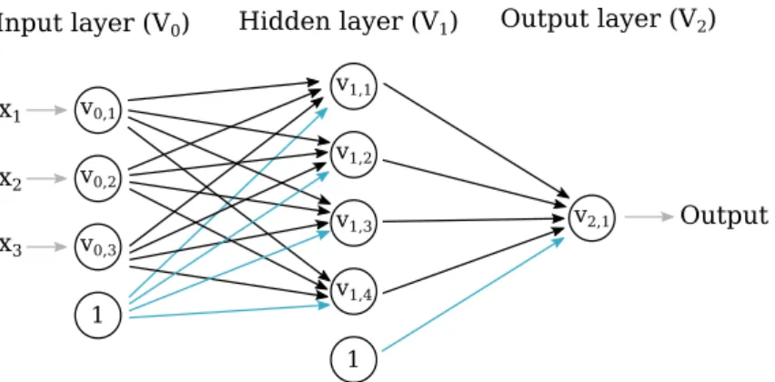
Feed-forward neural networks are directed acyclic graphs G = (V, E), with collection of neurons (as nodes) stacked in a layers, and a weight functionw:E −→R. An example of a feed-forward network is illustrated in Figure 1.

Every neuron computes a weighted sum of all its incoming edges and then applies a function to the computed weighted sum. An example neuron depicted in Figure2

calculates valueh as follows

h=σ(

4 X

i=1

xiwi+b) = σ(x.w+b)

where σ(.) is a non-linear activation function, w= (w1, w2, w3, w4)T is a weight

vector in correspondence with the incoming edges, and b is the neuron’s bias. The weights of all edges are the parameters to be learned. And the weights of the blue edges are called bias. Each neuron has its own bias as depicted in Figure

1. Every neural network is composed of at least one input layer, one output layer and an arbitrary number of hidden layers. The input layer is where a data point is fed into, with each neuron in the layer accounting for all dimensions of the data point. The output layer is tailored according to the task at hand; for instance, if we want to predict a scalar label y∈R, there would be one neuron in the output layer, determining probability of presence of each digit (0−9) of an image of a hand-written digit would require one neuron for each digit. The hidden layers, however, can have arbitrary number of neurons and the term “deep” in deep-learning is associated with

(19)

the number of hidden layers in a neural network. It is this existence of hidden layers that enables neural networks to learn non-linearly separable problems.

If we define the activation function of a single neuron to be the sign function we defined in Equation (3), it is not hard to see that this neuron would be an implementation the Perceptron algorithm described in Section 2.4. And for this reason, such neuron is called the “perceptron” neuron in the literature [5]. In practice the choice of the activation function is dependent on the nature of the problem being solved; for example, in multi-class or binary classification tasks where what is being predicted is a probability distribution over the class labels, it is common to use softmax and sigmoid functions respectively to approximate probabilities, due to their smooth and bounded (normalized in case of softmax) outputs [9]. However, these should not be the sole reasons why such functions are used to approximate probabilities; many other differentiable and normalized functions can be viable candidates. Nonetheless, both functions are commonly used in the last layer of neural networks to estimate probability distribution in practice.

Softmax in particular is derived from Boltzmann’s distribution, which is the maximum entropy (arg max_p(−P

ipilog2pi)) probability distribution that a system with temperature T occupies a certain state si, where each state has a different energy level i and a defined mean energy Pipii across all possible states:

pi = eβi

P

jeβj where coldness β = 1

kT and k is a constant. In many instances, e.g. Equation (38), parameter β is assumed to be equal to 1.

We will observe both softmax and sigmoid functions approximating probabilities in practice in Section 5.

The parameters of neural networks are the weights and biases that need to be learned. Given that the number of parameters are often inextricably large, calculating gradient of the loss function, which is needed for gradient based optimization methods such as stochastic gradient descent (SGD), becomes impractical. For this reason, back-propagation is used to calculate partial derivatives of loss function at each layer by going through layers backwards and employing chain rule to eliminate redundant calculations compared to direct calculation of gradient based on the general form of the loss function [10].

(20)

Input layer (V0) Hidden layer (V1) Output layer (V2) x1 x3 x2 v0,1 v0,2 v0,3 1 v1,1 v1,2 v1,3 v1,4 1 v2,1 Output

Figure 1: A feed-forward networks with one hidden layer. A data point x = (x1, x2, x3)T is fed into the network, for which a single label is produced by neuron

V2,1. The biases of the neurons correspond to the weights of the blue edges.

h

x

₁

x

₂

x

₃

x

₄

Figure 2: A computational neuron with four incoming edges. The output h is the weighted sum of all the incoming edgesx1, . . . , x4, passed to some non-linear function.

(21)

2.7 Dimensionality Reduction

Embedding high-dimensional graph-structured data into lower-dimensional vector spaces is the centerpiece of this thesis, which is at heart a dimensionality reduction procedure. Before diving into techniques for graph embedding, we study a much revered unsupervised learning algorithm for reducing the dimensionality of Euclidean data, namely the Principal Component analysis, PCA for short. We will observe how it bears resemblance to the well-known graph embedding techniqueLaplacian eigenmaps studied in Section4.

Dimensionality reduction is a technique of mapping high-dimensional data into a low-dimensional space, and so akin to the concept of lossy compression in infor-mation theory. In many cases, the high-dimensional data points might lie on a low-dimensional manifold and thus learning such a manifold would yield the said mapping. In fact, the terms ‘manifold learning’ and ‘dimensionality reduction’ are often used interchangeably for this reason [11].

There are several reasons to reduce the dimensionality of the data. From a compu-tational efficiency standpoint, manipulating high-dimensional data can be challenging. Furthermore, high-dimensional data can result in substandard generalization ability of the learning algorithms and in that sense, dimensionality reduction is said to have a de-noising effect [3]. More generally, dimensionality reduction can be used for extracting meaningful structures from the data and for visualization purposes.

Many dimensionality reduction algorithms have been developed, of which the perhaps most well-known is the Principle Component Analysis (PCA). PCA both compresses and recovers the data points by applying linear transformations and aims to find such transformations such that the differences between the original vectors and the recovered vectors are minimal. PCA can also be viewed in light of variance maximization. More specifically, transformations are such that the variance of the projected data points is maximal.

There are multitudes of algorithms that apply non-linear transformation such as Kernel PCA [12] and Laplacian eigenmaps [13]. The Laplacian eigenmaps will be reviewed extensively in Section 4.

2.7.1 Principle Component Analysis: Reconstruction Error Minimiza-tion

As said before, PCA is an unsupervised learning algorithm; that is the label set

Y is an empty set. The domain set X includes x1, . . . ,xN that are N column vectors (data points) residing in Rd. PCA aims to apply a linear transformation to reduce the dimensionality of the vectors from d to k where k < d. Let matrix W∈Rk×d _{represent the linear transformation which induces the mapping} _x_7→_Wx. So,Wx is inRk and is the lower-dimensional representation of the vectorx. Having defined the compression matrix, we define matrix U∈Rd×k _{to be the decompression} matrix that recovers vectorx from its compressed version in thek-dimensional linear subspace. That is, the reconstructed vector ˆxis equal to UWx and resides in the high dimensional spaceRd_.

(22)

Having written out the compressed and recovered vectors in mathematical terms, the PCA problem reduces to minimizing the reconstruction error in the least square sense. That is, we wish to find the matrices W and Ufor which the total squared distance between the original and reconstructed vectors among all the data points is minimized (which constitutes the loss function L)

arg min W∈_Rk×d_,_U_∈_Rd×k n X i=1 ||xi−UWxi||22 (10)

Additional to this error minimization perspective there is an alternative way to define PCA. We can also view PCA as finding projections which maximize the variance. More concretely, the first principal component is the vector in the original space along which the projections of the data points have the largest variance. The second principal component is the vector that maximizes the variance along all the vectors orthogonal to the first, and so on. We will see shortly how the variance maximization is mathematically equivalent to minimizing the reconstruction error. In the following lemma, we see that the solution to the Equation (10) takes a specific form.

Lemma 3 LetW and Ube the optimal solutions to Equation (10). Then W=UT and the matrix U is orthogonal; that is UTU is the identity matrix Ik in Rk

Proof: For any W and U, the mapping x 7→ UWx has the range R of k

dimensions, that is, it is akdimensional linear subspace ofRd_{. Such a space then must} have a corresponding matrix V∈Rd×k_{, whose columns are the orthonormal basis} vectors of this subspace—which is the new coordinate system—meaning VT_V₌_I_, with range R. Thus, any vector in this subspace can be written as Vzwhere z∈Rk_. The term Vz is viewed as the reconstructed vector in the original vector space of dimensional d from the low-dimensional representation vector z. The difference between the reconstructed and original vectors, for every z∈ Rk _and _x _∈_Rd_{, can} thus be written as follows

f(x,z) = ||x−Vz||2₂ =xTx+zTVTVz−2zTVTx=||x||2₂+||z||2₂+−2zTVTx Where we used the fact that VT_V₌_I

k. To find the vector z that minimizes the preceding expression, we compute the gradient with respect to z and set it to zero

∇zf(x,z) = 2z−2VTx= 0 =⇒z=VTx

Therefore, for every data point xwe can write VVTx= arg min

ˆ x∈R

||x−xˆ||

This provides a lower bound on the objective function stated in Equation (10). Thus

(23)

n X i=1 ||xi−UWxi||22 = n X i=1 ||xi−Vzi||22 ≥ n X i=1 ||xi−VVTxi||22

Since this inequality holds for everW and U, the optimal solutions for them are VT _and _{V, and this concludes the proof.}

The optimization problem stated in Equation (10) can thus be re-written as follows. arg min U∈_Rd×k_,_UT_U₌_I n X i=1 ||xi−UUTxi||22 (11)

The matrix UUT is the projection matrix whose columns are orthonormal. Specifically, UT_x

i is the projection ofxi onto the subspace spanned by the columns of U. And UUT_x

i is the reconstructed xi in the original coordinate system.

We further expand out the term in Equation (11)’s sum for everyx∈Rd _{and matrix} _U_∈

Rd×k _{such that}_UT_U₌_I _{as follows}

||x−UUTx||2 2 =x T_x₊_xT_UUT_UUT_x₋_2xT_UUT_x =||x||2₋_xT_UUT_x =||x||2₋_trace(xT_UUT_x) =||x||2₋_trace(UT_xxT_U) (12)

Minimizing Equation (12) is equivalent to maximizing the trace term since the length of vectors are given. So, the minimization problem in Equation (11) can be re-written as a maximization problem. Using the fact that trace is a linear operator, we now aim to solve the following optimization problem

arg max U∈_Rd×k_,_UT_U₌_I trace UT n X i=1 xixiTU ! (13) There are at least two ways to solve Equation (13) which are the spectral theorem and the Lagrange multiplier method. The former approach is what follows

LetM denote the matrixPN

i=1xixTi . The matrix Mis symmetric, as can be seen, and thus allows for the use of the spectral theorem and so can be written using its structural decomposition asM=VΛΛΛVT _{where the matrix}_V _{has the orthonormal} eigenvectors of M as its columns which in turn entails that VΛΛΛVT ₌_VT_Λ_Λ_ΛV ₌_I and the corresponding eigenvalues are along the diagonal of the diagonal matrix Λ

ΛΛ. We also assume that the eigenvalues are ordered in a descending order, that is ΛΛΛ11 ≥ ΛΛΛ22 ≥ . . . ≥ ΛΛΛdd. Moreover, M is positive semidefinite, meaning all its eigenvalues are non-negative. Having established these characteristics, we can study the following theorem that claims the solution to Equation (13), matrix U, takes a specific form.

Theorem 4 Given arbitrary vectors x1, . . . ,xN in Rd, let M=PNi=1xixTi , and let U be a matrix whose columns are the eigenvectors u1, . . . ,uk of M corresponding

(24)

to its k largest eigenvalue.Then, the solution to the optimization problem given in Equation (13) is matrix U and W=UT

Shalev-Shwartz and Ben-David [3] provide a solid proof using the spectral decom-position theorem:

Proof:We choose an arbitrary matrixU∈Rd×k _{whose columns are orthonormal} and letVΛΛΛVT _{be the spectral decomposition of matrix} _{M. Additionally, we define} matrix B to be VT_{U. Then,} _VB₌_VVT_{U. Given that matrix} _V _{is an orthogonal} matrix we haveVB=U and consequently the following equality also holds

UTMU=BTVTVΛΛΛVTVB=BTΛΛΛB

Where BT_B ₌_I_{, meaning its columns are orthonormal. Then, we can write out the} trace of the resulting matrix as

trace(UTMU) = d X i=1 Λii k X j=1 B_ij2

We attempt to exploit a square matrix instead ofBto provide an upper bound on the trace value. Let’s define ˆB to be inRd×d _{whose first}_k _{columns are that of}_B _and to also be orthogonal, that is ˆBT_B_ˆ _{= ˆ}_B_B_ˆT_{. The orthogonality of matrix ˆ}_B_{allows us} to have Pd

j=1Bˆij2 = 1 for every rowi, which in turn implies that

Pk

j=1Bij2 ≤1. So, given these, and the fact thatPd

i=1 Pk

j=1Bij2 = k, we can assimilate a vector into the the right-hand side of the equation above to capture the characteristics just derived, providing an upper bound for the trace value

trace(UTMU)≤ max b∈[0,1]d_:_||_b_||≤_k

d

X

i=1

Λiibi

The right-hand side of the equality above is simply a weighted sum of the d

largest eigenvalues of matrix M. Noting that the sum of elements of the vector b

must be less than or equal tok and the eigenvalues are along the diagonal of ΛΛΛ in a descending order by assumption without loss of generality, the maximum is achieved when the first k elements are set to one and the rest to zero, that is Pk

i=1Λii. Thus, for any matrix U∈Rd×k _{with orthonormal columns we have}

trace(UTMU)≤

k

X

i=1

Λii

If we placeUby the matrix whose columns are thek eigenvectors ofM, corresponding with the k biggest eigenvalues we get

trace(UTU | {z } I Λ ΛΛ) = k X i=1 Λii Therefore, we observe that trace(UT_{MU) =}Pk

i=1Λii whenU’s columns are the k leading eigenvectors ofM and the proof is concluded.

(25)

The PCA algorithm is summarized in Algorithm 3. We construct M in time

O(N d2_{) and compute its eigendecomposition in} _O₍_d3_{) and so the computational}

complexity of PCA isO(N d2₊_d3₎

Algorithm 3: PCA(x₁, . . . ,xN, k) Input: N data points x₁, . . . ,xN number of principal components k

Output: k principal components u1, . . . ,uk Compute M=PN

i=1xixiT

Compute k eigenvectors u1, . . . ,uk of M corresponding to the k largest eigenvalues subject to uT

i uj = 0 for alli6=j and ||ui||= 1 for all i return u₁, . . . ,u_k;

2.7.2 Principle Component Analysis: Variance Maximization

We observed that PCA optimization problem was formed out of minimizing the reconstruction error in the previous section. However, an alternative approach comes into light when we attempt to decipher what the maximization problem in Equation (13) signifies. We start by discerning what the matrix Pn

i=1xixTi represents. We calculate the expectation of each dimension of the data points, that isµµµ= _n1 Pn

i=1xi, that is in Rd. If we subtractµµµ from each data point, the matrix becomesPn

i=1(xi−µµµ)(xi−µµµ)T. This new matrix divided by n yields the covariance matrix. Therefore, the original matrix Pn

i=1xixTi is in fact the covariance matrix of thecentered data points times constant n. Centering the data points is referred to the act of subtracting the mean from the data points so as to make the mean zero, which is a common practice to do prior any calculation. Now that we have established matrixM is in fact the covariance matrix of the data points, we begin to look at the PCA problem from a different perspective.

PCA can be formulated as finding a different coordinate system for the data in which the variance of the data is maximized. Let xi ∈Rd be a data point and u ∈ Rd _{a basis vector of the new coordinate system. The projection of} _x

i ontou is the their dot product uT_x

i assuming ||u|| = 1. What we would like is for the variance of the projections of xi for i= 1, . . . , N to be maximum. Recalling what variance mathematically is and assuming that the data points are centered, i.e. their mean is zero, the variance of the projections is as follows

(26)

1 N N X i=1 uTxi 2 = 1 N N X i=1 uTxi xTi u =uT 1 N N X i=1 xixTi u

we substitute in the matrix U∈Rd×k _{whose columns are the new orthonormal} basis vectors, as well as the covariance matrix Σ in place of _N1 PN

i x_ixT i to arrive at the following optimization problem

arg max

U∈_Rd×k_,_UT_U₌_I

traceUTΣU (14)

Equation (14) chooses a new coordinate system of k(k < d) dimensions spanned by columns ofU such that the total variance of the projected data points, that is the sum of the variance of each dimension d, is maximized. We already observed in Theorem 4 that the solution to this optimization problem is given by first k

eigenvectors, arranged in an ascending order, of what we now know as the covariance matrix.

TheLagrange multipliersis an alternative way to deduce the same conclusion. For the sake of simplification, we assume we would like to find the variance of projections onto a single vector u. The constrained optimization method is thus

maximizeuTΣu s.t. ||u||2 _{= 1}

We will see in Section 4 that this term is called the Rayleigh quotient—of the co-variance matrix—and yet another perspective is introduced that deduces eigenvectors are solutions to maximizing/minimizing such terms.

We use the Lagrange multiplier λ to combine the constraint with the function to be maximized [14]

maximizef(u, λ) =uTΣu−λ(uTu−1)

We solve for u by finding the stationary point of the above function, that is differentiating with respect to u and equating it to zero

∂f(u, λ) ∂u = 2u T_Σ₋₂_λ_uT _{= 0} uTΣ = λuT (uTΣ)T = (λuT)T Σu=λu

(27)

And we have therefor arrived at the eigenvector equation of the covariance matrix

σ. Thus, for k biggest eigenvalues λ1 ≥ . . . ≥ λk ≥ 0 of covariance matrix Σ, u1

gives the orientation of the largest variance, u2 gives the orientation of the largest

variance orthogonal to u1 (the second largest variance), all the way to uk that is orthogonal to all the other eigenvectors, achieving the least variance among.

Therefor, we validated that the variance maximization and reconstruction error minimization in PCA are mathematically equivalent.

(28)

3 Introduction To Graph Embedding

Graph embedding methods aim to learn vector representations, embeddings, for the vertices of a graph. The goal is to produce an embedding for each of the vertices of the graph in a way that capture the graph topology, node-to-node relationship, or some relevant information of interest regarding each nodes, the graph, or the subgraph. The geometric relations in the latent space, where nodes are projected into, correspond to relations among them (e.g. links) in the original graph [15].

The low-dimensional embeddings represent the high-dimensional non-Euclidean graph-structured data and can be subsequently used for downstream tasks, such as community detection and link prediction.

Goyal and Ferrara [16] abstract the applications of graph embeddings into four categories: node classification, link prediction, clustering, and visualization. So we may be interested in determining labels of vertices of a partially labeled graph [17], to predict missing links between vertices [18], or to cluster similar nodes together [19]. A multitude of methods exists for such applications. For node classification there are methods that extract features from the graph vertices to subsequently feed them into a classifier [20], or methods that exploit random walks to propagate the labels [21]. Among approaches for link prediction exist maximum likelihood models [22] or similarity measure [23].

3.1 Definition and Preliminaries

3.1.1 Definition of Graphs and some of their Associated Matrices Let G= (V, E) be a graph that is a collection of vertices (nodes) represented by the setV ={v1, . . . , vn} and edges (links) among them represented byE ⊆ V × V.

The adjacency matrix of a graph is denoted by A ∈ R|V|×|V| _{whose elements} are 1 or 0, representing existence of edges among the vertices. More concretely

Aij = 1 if (vi, vj) ∈ E otherwise Aij = 0. For a weighted graph, however, a non-negative weight is associated with every edge in graph and the adjacency matrix is directly translated into aweight matrix—a.k.a. weighted adjacency matrix—W where Wij ≥0 ∀i, j ∈[n]. If nodes vi and vj are not connected thenWij = 0

We assume that the graphs are undirected—unless stated otherwise—, that is if (vi, vj) ∈ E then (vj, vi) ∈ E. In such graphs we may use the set notation

{vi, vj} ∈ E instead of the tuple. And the corresponding adjacency or weight matrices are symmetric, that isWij =Wji ∀i, j ∈[n].

The edge wights Wij are generally studied as a measure of similarity between nodesvi and vj and the higher it is, the more similar the two nodes are presumed to be [16].

For an unweighted undirected graph G, the degree of a vertex vi, denoted by di, is defined as follows di = n X j Aij

(29)

In case of a weight matrix this is directly translated into the following di = n X j Wij

This gives way to another matrix associated with graphs called the degree matrix D. The matrix D is a diagonal matrix that has the degrees d1, . . . , dn along its diagonal and 0 elsewhere.

3.1.2 Graph Embedding: An Encoder-decoder Framework

We try to put the concept of graph embedding1 introduced thus far on a concrete and unified footing by shedding light on the encoder-decoder framework, proposed by Hamilton et al. [24].

Two key components of the framework are two mapping functions: an encoder and a decoder. The idea is for the model to be able to learn high-dimensional information about the graph—such information can be the structure of local graph neighborhoods of nodes, or classification labels for the nodes [17]—from the low-dimensional embeddings of nodes. To this end, the encoder should map each node to a low-dimensional vector, and the decoder should decode the structural information of the graph from the learned embeddings. In principle, the embeddings should suffice to provide all the needed information for the subsequent off-the-shelf machine learning algorithms. The encoder and decoder are functions as follows.

ENC :V →Rd ₍₁₅₎

DEC :Rd×Rd _→_R+ ₍₁₆₎

The encoder takes node vi ∈ V as an input, and outputs the associated embedded vector zi ∈Rd. The decoder, on the other hand, takes two embeddings as inputs and outputs some similarity measure. This measure could be any user-defined similarity measure, e.g. the shortest path length between the two nodes [25] or the existence of an edge [26]. [24] claims that although numerous decoders are possible, in most instances in the literature decoders take the aforementioned pairwise form. In 3.2.3

we will see an approach where a unary decoder is used.

The course of action is therefore as follows. The encoder embeds input nodes of the original graph vi and vj and outputs the corresponding embeddings, zi and zj respectively. The two embedded vectors are then passed to the decoder. The decoder, thereafter, reconstructs a similarity measure between the pair of nodes vi and vj in the original graph. The problem is then turned into the optimization of the encoder-decoder model to minimize the error in the reconstruction so that

DEC(ENC(vi), ENC(vj))≈sG(vi, vj) (17)

1_{The term graph embedding is referred to the embeddings of the vertices of graphs throughout.} However, in the literature, sub-graphs can also be embedded, as discussed in [24].

(30)

sG :V × V 7→R+ 2 is a similarity measure between the nodes of the graph and can thus be represented as asimilarity matrix S∈R|V|×|V|_{. The similarity matrix is} user-defined, examples of which include the adjacency matrix [26], sG(vi, vj),Ai,j, or the probability of two nodes co-occurring in a fixed-length random walk over G

[27, 28].

Many approaches of graph embedding differ in how they define similarity matrices. [16] states two different measures:

• First-order proximity

Because edge weights provide the most primitive similarity measure between nodes, they are also named first-order proximity. An example of such weight is illustrated by Equation (20).

• Second-order proximity

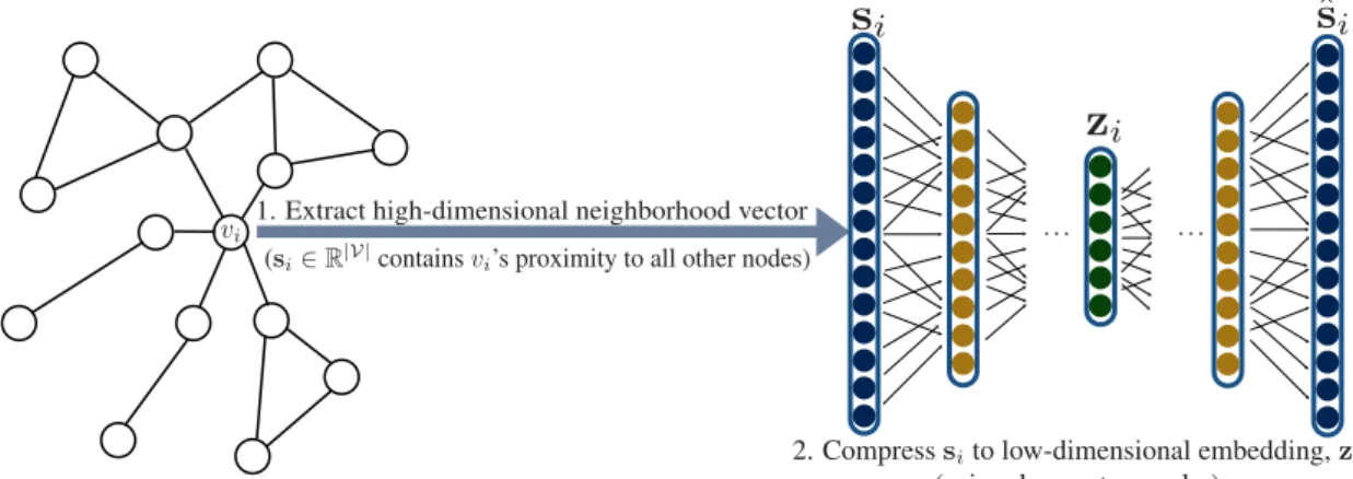
Second-order proximity provides measure of similarity of the neighborhoods of nodes. More specifically, if we denote row iof matrix S bysi, such vector would yield the similarity measure of vertex vi with all other vertices, that is si = (Si1, . . . , Si|V|)T. The second-order proximity of nodes vi and vj is thus given by the similarity of si and sj. Examples of higher-order proximity measures include Common neighbors, or Katz Index, etc. [29]. Techniques such as [27, 28] preserve high-order proximity among nodes.

The next building block is the bedrock of the learning paradigm: a user-defined loss function,` :R×R→R, that measures the discrepancy between the estimated and the true similarity measure between all pairs of nodes. The empirical loss function is thus to be minimized over all the pairs of nodes in the training setS

L= X

(vi,vj)∈S

`(DEC(zi,zj), sG(vi, vj)) (18) Minimizing the loss function in Equation (18) results in a trained encoder-decoder model. The model can then be used to output embeddings for the nodes. The resulting latent features may be fed into downstream machine learning algorithms to, for instance, classify node labels or perform link predictions.

The four primary methodological components of graph embeddings discussed thus far can be summarised as follows.

1. A similarity matrix, S, that describes a notion of user-defined similarity between the nodes of graph G—or the neighborhoods of the nodes.

2. An encoder function, ENC, that encodes the nodes into latent vector representations, i.e. embeddings. Usually most of the parameters of the model that are parameters of the in the encoder function.

3. A decoder function, DEC, which estimates the pairwise similarity measures from the generated embeddings and usually has no trainable parameters [24].

(31)

4. A loss function L, that quantifies the quality of the reconstructed pairwise similarity measures with the help of true similarity measure function sG. The existing graph embeddings differ primarily in how they define these four components, two examples of which we will observe in Section 4 and Section5

3.2 A Taxonomy on Algorithmic Approaches

Initially, graph embedding algorithms were developed as a means to reducing the dimensionality of the data [16]. A powerful approach is Laplacian eigenmaps method [13]—which we will extensively study in Section4—where a graph is constructed that encodes some similarity notion amongN d-dimensional data points. The data points are then embedded in a lower-dimensional vector space, preserving the proximity of the vertices of the graph. These methodologies however lack scalability given they often operate in time quadratic in dimensionality of the data O(d2_).

More scalable methodologies lean more towards random walk based methods—of which Deepwalk [28] will be discussed in Section 5— or neural networks as studied in [30] that both captures the non-linear structure of the graph and leverages the sparsity of real-world graphs.

There has been a surge in survey papers on the topic, among which are [24, 16] that we will explore to present an overview of the existing taxonomy on graph embedding technique.

Goyal and Ferrara [16] categorize the existing graph embedding techniques into three broad categories: factorization based techniques, random walk based methods, and deep learning based approaches. Hamilton et al. [24] provide a slightly different taxonomy in that embedding can take place at two different scales of (1) embedding nodes or (2) embedding sub-graphs. Among the node embedding techniques, they introduce two categories of deep neural networks, and shallow embedding within which factorization based methods and random walk-based approaches fall.

3.2.1 Factorization based methods

Factorization based algorithms, inspired by classic dimensionality reduction tech-niques leverage the connection of graphs and matrices. More broadly, spectral graph theory aims to explore graphs through the lens of eigenvectors and eigenvalues of matrices naturally associated with graphs. These matrices, namely adjacency matrix, Laplacian matrix, etc. can be factorized to obtain node embeddings. The techniques used to factorize the representative matrices differ depending on the properties of the matrices. In Section 4we will study an example of factorization-based method that leverages eigenvalue decomposition of the Laplacian matrix.

3.2.2 Random Walk based Methods

Random walks are exclusively useful when graphs are too large to be studied in their entirety. The sampled random walks from the graph are to approximate the structure of the whole graph and therefore prove to be scalable. Deepwalk, a proposed random

Learning Embeddings for Graphs and Other High Dimensional Data

Preface

Contents

1

Introduction And Outline Of The Thesis

2

Machine Learning

2.1

Notation

2.2

A Formal Mathematical Learning Model

2.3

Empirical Risk Minimization

2.4

The Perceptron Algorithm: A Linear Classifier

2.5

Generative Models

2.6

Artificial Neural Networks

h

x

x

x

x

2.7

Dimensionality Reduction

3

Introduction To Graph Embedding

3.1

Definition and Preliminaries

3.2

A Taxonomy on Algorithmic Approaches