Munich Personal RePEc Archive
Investigating the Government
Revenue–Expenditure Nexus: Empirical
Evidence for the Free State Province in a
Multivariate Model.
Omoshoro-Jones, Oyeyinka Sunday
Free State Provincial Treasury, Bloemfontein, South Africa
27 March 2020
Online at
https://mpra.ub.uni-muenchen.de/101349/
1
Investigating the Government Revenue–Expenditure Nexus: Empirical
Evidence for the Free State Province in a Multivariate Model.
Oyeyinka S. Omoshoro-Jones
Ecoonomic Analysis Directorate, Department of Free State Provincial Treasury, Bloemfontein, South Africa, 9301.
Abstract: This paper examines the government revenue–expenditure nexus for the Free State Province in a multivariate modelling framework using real GDP and inflation as control variables over the period 2004Q2–2018Q1. Cointegration and intertemporal (causal) links among variables were established employing Johansen-Juselius (1990) within a vector error correction model (VECM) and Toda-Yamamoto (1995) non-Granger causality test. Cointegration analysis affirms the existence of a long-run relationship between variables. The results of the causal analyses show a bidirectional causality between government revenues and expenditures in both the long-run and short-run, supporting the fiscal synchronization hypothesis. Real GDP and inflation individually Granger-causes government revenues in both the long-run and short-run, stressing their importance on generating revenue. Based on these findings, an isolated fiscal measure to raise tax-revenues or cut expenditure will exacerbate fiscal imbalance. The Free State government through its provincial treasury should adhere to a planned budget process, devise innovative revenue-generating strategies to circumvent the burden of producing inflation revenue, and effectively use its autonomy on fiscal instruments to maintain a sustainable fiscal policy path and stimulate economic activity level.
Keywords: VECM, Expenditure, Revenue, Causality, Cointegration, Free State province.
JEL Classification: C12, C51,C54, H61. 1. Introduction.
In the aftermath of the latest global economic and financial crisis, the South African government have been grappling with an expanding fiscal debt (as a ratio of GDP) due to government expenditures outpacing tax-revenues (Figs. 1 and 2 in the Appendix), while economic growth is constrained with structural endogenous shocks (e.g., shortage of power supply), political uncertainty, weak global demand for commodity export and gyrations in the world capital market. At the same time, the labour market condition has steadily worsened in the past decade1. The combined effects of these developments require the national government to design/ implement effective economic and fiscal policies to tackle these socioeconomic issues and stimulate economic growth (see, e.g., NDP, 2012; NGP, 2011). While, in political and academic discussions, there is a growing concern over South Africa’s ever-increasing fiscal debt utilized to finance the rise in government expenditures, which in turn widen budget deficit (National Treasury, 2020).
Intuitively, the narrowing fiscal space, severely weak economic growth and relatively low tax-revenues may affect the national government’s allocations (i.e., equitable shares2) to provinces directly or indirectly. Hence, provincial governments are often confronted with the dilemma of either reducing public spending or utilize their fiscal autonomy to raise “own revenue” to augment their provincial
1South Africa’s fiscal debt (as % of GDP), a key measure of national government’s indebtedness and financial
health has nearly doubled in size from 31.8% in 1990 to 59.3% at the end of 2019 (National Treasury, 2020), even as its economic growth drastically slowdown to about 0.7% at end of 2019 from the recorded 4.2% in 2000 (IMF, 2020).The country is also experiencing a persistently high unemployment rate at 29.1% (narrowed definition) or 42.3% (expanded definition) at the end of 2019 (StatsSA, 2020).
2South African uses an intergovernmental fiscal framework, in which, collected tax-revenue by the national
government are allocated as equitable shares (to fund both earmarked and conditional grants) across the nine provinces based on set of criterion.
2 equitable share (PES). Nevertheless, a key question is which of these budgetary components will actually foster fiscal sustainability or restore fiscal balance?. The answer to this question cannot be based on a priori judgement but it remains an empirical issue.
In South Africa, the provincial governments receive a large fraction of their revenue (i.e., PES) from the national government in the form of intergovernmental transfers which are mostly devoted to financing flagship programmes or projects identified by the national government to show its political commitment to the voters, on tackling income inequality, unemployment and poverty rate. This gives the assumption that provincial governments operate under a balanced budget, which becomes questionable due to off-budget activities deemed as the main priority in a particular province (Payne, 1998). In this context, the fiscal autonomy of the provincial governments becomes crucial to generate extra revenue to fund off-budget activities (or provincial financial priorities) by either raising levies and surcharges3. Albeit, a priori decision by the policymakers either to raise tax-revenue or cut expenditure to finance current spending (or budget deficit) can lead to serious budget constraints which may indirectly dampen economic activity level or induce inflationary pressures in the domestic economy.
However, a better understanding of the dynamic interrelationship between government revenue and expenditures would aid policymakers to pin down the causes of, and remedies for, non-credible budget. From a policy standpoint, such knowledge could also be useful in designing and/or implementing appropriate fiscal measures to improve the budget planning process, achieve fiscal sustainability and reduce budget deficit. Besides, it is widely accepted that sound fiscal policy can promote price stability and sustain growth in output and employment. As a policy tool, it can reduce output and employment fluctuations in the short-run, and also restore the economy to its potential level. This present study contributes to the extant literature investigating the causal relationship between government revenues and expenditures at the state level, by focusing on the temporal interdependence between the two variables in the domestic economy of the Free State (FS) province over the period over the period 2004Q2–2018Q1 employing the vector error correction modelling approach and VAR-based non-Granger causality test developed by Toda-Yamamoto (1995), together with real gross domestic product (GDP)4 and inflation as control variables within a multivariate framework.
This empirical analysis is timely and important in at least on two counts. Firstly, the economic and labour market conditions in the FS province mirrors that of the national economy given a relatively high unemployment rate of 35% (narrow definition) or 37% (expanded definition) at the end of 20195, and a lacklustre domestic economy that recorded negative growth of -0.3% in 2019 compared to the growth rate of 2% and 2.5% in 2000 and 2010 respectively6. Premised on this reality, the provincial government is faced with the daunting task of resuscitating the provincial economy and concurrently reduce the prevailing high rate of unemployment and poverty rates with the limited available financial resources which constitute the bulk of the equitable shares allocated by the national government.
On the other hand, the enforcement of stringent fiscal consolidation measures by the South African government, to reduce the increasing fiscal debt, budget deficit, wasteful expenditures and public wage bill, has an unintended indirect effect on the Free State’s equitable share, while the increasing off-the budget activities to ameliorate the impact of the emergent dire socioeconomic conditions makes the provincial budget fiscally unsustainable. Given the current socio-economic and fiscal challenges; the Free State government is obliged to use its fiscal autonomy to explore innovative measures to either generate more revenue to finance the provincial needs or reduce its expenditures to achieve fiscal balance. Hence, the findings on the underlying dynamic interrelationship between government revenues and expenditure will shed more light on whether the conventional fiscal measure to raise tax-revenues (on levies and surcharges) or cut expenditures or concurrently use both measures will revive the provincial economy as well as mitigate budget constraints due to higher expenditures and low revenue (Fig.3 in the Appendix).
3Levies and surcharges are other form of taxes used by the provincial (or state) government as fiscal tools to raise
‘own’ revenue. Note, the provincial ‘own’ revenue is referred to as government revenue from Sections 3 to 6.
4Note, GDP variable that is used in our analysis refers to the GDP-R that measures the provincial economic
growth, calculated and published by the Statistics South Africa (StatsSA).
5See, StatSA’s published Quarterly Labour Market Survey for 2019:Q4.
3 Secondly, the relationship between government revenues-expenditures empirically rests on four hypotheses in the public finance literature7, which includes (i) tax-spend, (ii) spend-tax, (iii) fiscal synchronization, and (iv) institutional separation. While the first three hypotheses imply interconnection between government revenue and expenditures (see, e.g. Friedman, 1978; Buchanan and Wagner, 1979; Musgrave, 1966; Meltzer and Richard, 1981), the institutional separation hypothesis suggests an independent relationship between these budgetary components (Wildavsky, 1988; Baghestani and McNown, 1994). These theories have different policy implications. This, it is imperative for both the fiscal authorities and policymakers in the Free State province to have in-depth knowledge of the exact theoretical relationship underlying the government revenue-expenditure nexus in the province. This rationale lends credence to the relevance of the empirical investigation in this paper. Concrete evidence on the theory underpinning the revenues-expenditures nexus in the Free State will be useful to the fiscal authorities and policymakers in designing (or implementing) effective fiscal measures to finance other provincial priorities.
This paper also contributes to the extant literature in several dimensions. So far, only a few studies have examined the causal relationship between government revenue and expenditures in South Africa from the national government perspective (see, e.g., Chang et al.2002; Narayan and Narayan, 2006; Lusiyan and Thorthon, 2007; Nyamongo et al.2007; Ghartey, 2010; Ndahiriwe and Gupta, 2010; Baharumshah et al.2016; Phiri, 2019), however the same empirical research on the provincial economy8 remain scarce. To the best of our knowledge, our study is the first attempt to explore this line of empirical inquiry at the sub-national sphere of government in South Africa.
Furthermore, the findings in the existing literature for South Africa is inconclusive, as authors report contradictory evidence supporting a unidirectional causality running from government expenditures to revenue (see, Chang et al.2002); no temporal causal link between variables, indicative of fiscal neutrality (Narayan and Narayan, 2006) and bidirectional causality between variables (see, e.g., Phiri, 2019; Baharumshah et al.2016; Ghartey, 2010; Lusiyan and Thorthon, 2007). Thus, it is difficult for policymakers to design and/or implement effective fiscal measures to reduce the budget deficit or achieve fiscal sustainability in South Africa. Aside from, the different econometric techniques used in earlier studies and time-periods examined; the mixed results reported in most of the earlier studies can be attributed to cointegration and causality analyses were carried out in a bivariate framework which suffers from the omitted variable problem (see, e.g., Payne, 2003; Baghestani and McNown, 1994; Ashan et al. 1992; Signh and Sani, 1984, Lutkepohl, 1982); widespread use of low frequency (annual) data, as opposed to high-frequency data, has been proven to obscure the existing causative links between revenue and expenditures (Ndahriwe and Gupta, 2010); and structural breaks are often unaccounted for in the annual data used (save for Phiri, 2019; Lusiyan and Thorton), despite the increasing exposure of South Africa to globally transmitted shocks due to the country’s well documented increasing integration into the world economy and financial markets since 1994. Likewise, several fiscal measures have been adopted to encourage fiscal discipline and financial management at the national, provincial and municipal levels9.
Broadly speaking, the shortcomings in these earlier studies can lead to erroneous conclusions and fiscal policy formulation, given that the relationship between government revenue and expenditure may have changed because of the close link between business cycles and the budget working via automatic fiscal stabilizers and discretionary fiscal measures (Ewing, 2006:191), thus the failure to determine possible endogenous breaks (and deterministic trend) in the revenue and expenditure series can produce spurious results and conclusion on causal links (Islam, 2001).
7The different tax-debate theories, empirical evidence and policy implications are discussed in subsequent section
of this paper.
8Note, South African provinces are analogous to states in other countries/regions. See, e.g., Saunoris (2015), Payne
(1998), Marlow and Manage (1987) and Von Furstenburg et al.(1986) for studies investigating the government revenues-expenditures nexus at the state levels. See, also Payne (2003) for few studies that focused on the temporal relationship between government revenues and expenditures at the state and local government (municipality) levels.
9 Enacted financial regulations, most notably Public Finance Management Amendment Act (PFMA), No. 29 of
4
Most closely related to our work is Kavase and Phiri (2018), who investigate the fiscal sustainability across the nine South African provinces focusing on the existing asymmetric relationship between government revenue–expenditure. Even so, the drawn inferences and conclusion of this particular study can be considered as unreliable since the analytical exercise is performed in a bivariate model using high-frequency data that covers the period 2000 to 2016. Also, the short time-period covered in this study makes it susceptible to misspecification bias due to insufficient degrees of freedom, required to construct the optimal number of lags for times-series included in the non-linear autoregressive model (NARDL) used.
The methodology and model specification employed in this study circumvent the limitations of earlier studies. Specifically, our causality analysis is carried out in a multivariate cointegration-based error correction model using high-frequency data (i.e., quarterly series) with real GDP and inflation as control variables, to effectively deal with misspecification bias associated with omitted variable problems and spurious conclusions on the nature and direction of causality. Foremost, the cointegration-based error correction model employed allows feedback between government revenue and expenditure running interactively through the real GDP and inflation variables in both the short-run and long-run (Granger and Lin, 1995; Johansen and Juselieus, 1990). Second, the error terms from the long-run regressions between government revenue, expenditure, real GDP and inflation can give more insight into how, for instance, responsive revenues and expenditures are to deviations from their long-run equilibriums with respect to GDP. It is worth noting that the inclusion of the provincial real GDP in our model is due to the fact that the provincial government ‘own’ revenue and expenditure growth are intrinsically linked to the aggregate economic conditions in the province. Finally, the novel Toda-Yamamoto non-Granger causality test used in our analysis provides a reliable robustness check for the results of the estimated vector error correction models on the long-run relationship among variables. All in all, our drawn inferences and conclusion on both the linear and temporal causative links among variables are expected to be more robust than those reported in earlier studies.
The remainder of this paper is structured as follows: Section 2 provides the different theories explaining the government revenue-expenditures nexus, empirical evidence supporting these theories, and a synoptic survey of relevant studies. Section 3 outlines the econometric techniques employed. Data and stationarity properties of the time-series are presented in Section 4. Empirical results are reported and discussed in Section 5, while Section 6 concludes with some policy recommendations.
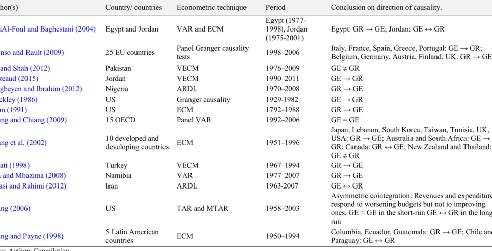
2. Theories on Government Revenues–Expenditure Nexus and Empirical Evidence. In public finance, four theoretical postulations underpin the government revenue–expenditure nexus (or the tax-spend debate) and important for the formulation of fiscal policy, these include: (i) the tax-spend, (ii) spend-tax, (iii) fiscal synchronization and (iv) institutional separation. A bird’s eye view of the burgeoning empirical literature validating these theories is provided in this sub-section, and relevant empirical studies are presented in Table A1 in the Appendix. See, for example, Payne (2003) and Phiri (2019) for a much broader survey of the empirical literature.
Friedman (1978) and Buchanan and Wagner (1997) are the main proponents of the tax-spend theory, arguing that changes in government revenues (taxes) leads to changes in government expenditure, from an opposing viewpoint. According to Friedman (1978), an increase in government revenues will directly raise government expenditures, implying a positive relationship between the variables. For example, the conventional fiscal measure to reduce budget deficits by increasing tax-revenue will exert an inflationary effect on goods and services, which raises government consumption expenditure. On this basis, lower taxes would reduce the budget deficit or engender fiscal sustainability (Darrat, 2002; Payne, 2003). On the contrary, Buchanan and Wagner (1997) posit a negative intertemporal relationship between government revenue and expenditure. Here, an increase in government revenue (or tax) will reduce the budget deficit, since voters will perceive a reduction in tax revenue as a decline in public spending, leading to increasing demand for public goods and services. Thus, increases in tax revenues combined with spending cuts will lower budget deficits. Empirically, a unidirectional causality from government revenues (or taxes) to government expenditure confirms the tax-spend thesis. The tax-spend hypothesis has been supported by the following empirical studies, to mention a few: Manage and Marlow (1986), Ram (1988), Bohn (1991), Owoye (1995), Ross and Payne
5 (1995), Payne (1998), Park (1998), Ewing and Payne (1998), Daratt (1998), Narayan and Narayan (2006), Kollias and Paleologou (2006), Wolde-Rufael (2008), AbuAl-Foul and Baghestani (2004), Eita and Mbazima (2008), Aregbeyen and Ibrahim (2012), Sennoga (2012), Magazzino (2013), Rahman and Wadud (2014), and Obeng (2015).
Tuning to the spend-tax theory, government spend first and raise revenue (taxes) later, which is the opposite of the tax-spend thesis. Peacock and Wiseman (1961, 1979) advanced spend-tax theory, arguing that the occurrence of idiosyncratic shocks (e.g., natural disaster, droughts) economic, social and political upheavals typically leads to higher taxes initially used to finance the required increase in government expenditure. This postulation is akin to Ricardian equivalence proposition by Barro (1974, 1978) suggesting that the present borrowing by government results in an increased tax liability in the future, hence government expenditure is fully capitalised by the public in recognition of these increased future tax liabilities. Empirically, the spend-and-tax hypothesis holds if a unidirectional causality from government spending to government revenue (taxes) exists and is known as the ‘displacement effect’. The spend-tax theory has been supported by the work of, for example, Blackley (1986), Von Furstenburg et al. (1986), Jones and Joulifain (1991), Payne (1998), Afonso and Rault (2009), Magazzino (2013), Chang et al. (2002), Narayan and Narayan (2006), Saunoris and Payne (2010), Keho (2011), Paleologou (2013), Kaya and Şen (2013), Ritcher and Dimitrios (2013), Nwosu and Okafor (2014), and Tiwari and Mutascu (2016).
Whereas, Musgrave (1966) and Meltzer and Richard (1981) put forward the fiscal synchronization hypothesis, maintaining that government expenditures and taxes can be adjusted simultaneously (or concurrently) to achieve fiscal balance (or equilibrium) given that policymakers have full control on both variables during budget adjustments. In theory, concurrent decisions on the appropriate government expenditure and tax revenues are imperative to optimize a community’s intertemporal social welfare function in a democratic society, as decisive voter also compares the marginal benefits and costs of initiated government programmes (Musgrave, 1966:19). Conversely, preferences of a community would determine the quantity and quality of public goods that government expenditure caters for, implying that the welfare-maximising choice of a decisive voter influence government expenditure level (or size), while the decisive voter chooses the tax share (Meltzer and Richard, 1981:924).
Therefore, the government can simultaneously choose an optimal package of public programmes to be financed in its budget along with tax revenues required. Since government expenditure and revenue are independent of each other, budget deficit can be reduced by raising taxes and reducing expenditure since both variables can be changed concurrently. Empirically, a bidirectional (or contemporaneous feedback) causality between government revenues and government expenditures validates the fiscal synchronization theory. Hence, an isolated fiscal decision to raise government revenue or expenditure will lead to a serious budget deficit, if contemporaneous feedback exists between the two variables. Empirical evidence on fiscal synchronisation theory have been reported by, for example, Manage and Marlow (1987), Miller and Rusek (1990), Owoye (1995), Payne (1998), Ewing and Payne (1998), Islam (2001), Chang et al. (2002), Kollias and Paleologou (2006), Lusiyan and Thorthon (2007), Nyamogo et al. (2007), Wolde-Rufael (2008), Chang and Chiang (2009), Ndahiriwe and Gupta (2010), Ghartey (2010), Mehrara et al. (2011), Elyasi and Rahimi (2012), Al-zeaud (2015), Takumah (2014), Baharumshah et al. (2016), Phiri (2019) and Raza et al. (2019).
Lastly, Wildavsky (1988) and Baghestani and McNown (1994) suggested the institutional separation hypothesis, under which decisions on government expenditure and taxation are taken independent of one another due to the conflicting views and interest of different parties or groups which causes fiscal debt to grow and makes it more challenging to implement deficit-reducing measures (Drazen, 2001; Persson et al. 2000). From a policy perspective, if institutional separation thesis holds, then fiscal consolidation out by raising tax revenues or cut in expenditure will not affect budget deficit (Lusiyan and Thorton, 2007:497). Empirically, no intertemporal causality between government revenue and expenditure is existing, and also referred to as fiscal neutrality. To mention a few, studies with findings on fiscal neutrality consists of the empirical work of AbuAl-Foul and Baghestani (2004), Narayan and Narayan (2006), Ewing (2006), Kollias and Paleologou (2006), Wolde-Rufael (2008), Zapf and Payne (2009), Magazzino (2013), Ali and Shah (2012), Masere and Kaja (2014), and Baharumshah et al. (2016).
6
2.1.Survey of related empirical studies
In the vast empirical literature, empirical studies examining the relationship between government revenue and expenditure in South Africa is scanty, while similar research at the provincial level receives no attention so far. Be that as it may, the findings of these studies remain mixed, partly due to model specification bias, different time period being studied, and econometric techniques used.
Some cross-sectional studies have considered South Africa in their analysis in a multivariate model by incorporating GDP as a control variable to deal with misspecification bias due to omitted variable problem (Payne, 2003). Most notably, Chang et al. (2002) employed the error correction modelling approach to assess the government revenue-expenditure nexus across ten developing economies using annual series, over the period 1951–1996 and finds a unidirectional causality running from government expenditure to revenue for South Africa in the short-run, supporting the spend-tax hypothesis. On the contrary, using the Toda-Yamamoto (1995) non-Granger causality test for twelve developing countries during the 1960–2000, Narayan and Narayan (2006) found no long-run causality between government revenue and expenditure in South Africa, keeping with the institutional separation (or fiscal neutrality) hypothesis. In a subsequent study, Ghartey (2010) utilised an ARDL model and the two-step Engle-Granger method to determine the direction of causality driving the government revenue-expenditure nexus in Nigeria, Kenya and South Africa using annual data spanning 1960–2007 and found a bi-directional causality among these variables for South Africa suggesting the existence of fiscal synchronisation hypothesis.
Similarly, few country-specific studies have considered the government revenue-expenditures nexus in South Africa. Among these, Lusiyan and Thorthon (2007) accounted for structural breaks by including dummy variables in bivariate model estimated for the period over the period 1895-2015 and established long-run relationship with the help of a VAR-based Johansen cointegration test. Their Granger-type causality tests suggest the existence of a bidirectional relation between revenue and expenditure, thus keeping with fiscal synchronisation hypothesis. Nyamongo et al. (2007) estimated a bivariate VAR model over the period October 1994 to June 2004 and reported a long-run bi-directional causality between government revenue to expenditure but without any evidence of temporal causal link which supports fiscal neutrality hypothesis.Ndahiriwe and Gupta (2010) argued that the mix results in the direction and nature of the causal relationship between government revenue and expenditure in South Africa can be attributed to the frequency of time-series used. Using both quarterly and annual together with GDP and government debt as control variables, the authors find bi-directional causality between revenue and expenditure only in the vector error correction model with quarterly data (1960Q1 to 2006Q2) but the result of a similar model with annual series (1960-2005) showed no evidence on the causative links among variables being studied.
More recent studies have utilized the asymmetric model to capture the non-linear features underlying government revenue and expenditure. In this strand of studies, Baharumshah et al. (2016) used annual data to estimate both asymmetric (i.e., threshold autoregression (TAR) and momentum threshold autoregression (MTAR)) and symmetric (error correction based-ARDL) bivariate cointegration models over the period 1960–2013 for South Africa and found no evidence of asymmetric cointegration among variables in both the TAR and MTAR, however, the results of the multivariate ARDL that make use of the GDP as control variable confirm that variables are linearly cointegrated in the long-run with bi-directional causality running from government revenue to expenditure, and vice versa in both the long-run and short-run.
Focusing on fiscal sustainability of South African provinces given the adopted strict fiscal consolidation stance by National Treasury, Kavase and Phiri (2018) employ the non-linear ARDL model to examine the asymmetry relationship behind government revenue–expenditure nexus across nine provinces over the period 2000–2016, and finds that the widespread strict fiscal stance to finance growing expenditure by raising taxes (increased revenue collection) has a differentiated long-run and short-run effects on provincial budgets, and widens the national fiscal debt given varying financial priorities in each province. These authors conclude that fiscal sustainability is attainable in both the long-run and short-run if government expenditures increased in Eastern Cape, Northern Cape and Free-State provinces but reduced in Western Cape, North West, Gauteng, Mpumalanga and Limpopo.
Finally, in a recent empirical work, Phiri (2019) make use of an asymmetric MTAR cointegration model supplemented with a TEC component with fiscal deficit/surplus (as a ratio of GDP) as a control
7 variable to examine the government revenue-expenditure nexus for South Africa over the period 1960Q1 to 2016Q2, and finds a bi-directional causality, in support of fiscal synchronization hypothesis.
3. Econometric Methodology: Cointegration-based Vector Error Correction Modelling This sub-section outlines the econometric approaches employed to examine the relationship between government revenue and expenditures in the Free State province. We begin with the construction of a hypothetical (functional) multivariate framework needed to study the existing linear and temporal relationships between provincial government ‘own’ revenue, expenditure and the two control variables. Next, we outline the cointegration based-vector error correction model and Toda-Yamamoto’s MWALD tests based on the developed functional model to carried out the causal analysis between variables.
3.1.Modelling Framework.
In the empirical literature, the assessment of the government revenue–expenditure nexus in a multivariate framework has been proven to produce more robust results and conclusion, compared to a bivariate modelling approach, which may obfuscate the direction and pattern of temporal links among variables, and misspecification bias associated with omitted variable problem (see, e.g., Payne, 2003; Lutkepohl, 1982)10. To this end, the underlying dynamically complex government revenue (GR)– government expenditure (GE) nexus is investigated at the sub-national level using provincial data by considering long-run linear stochastic equations within a multivariate framework as follows:
0 1 2 3 1 2 1
ln
GR
t
ln
GE
t
Y
t
t
g
t
d
t
t (1)0 1 2 3 3 4 2
ln
GE
t
ln
GR
t
Y
t
t
g
t
d
t
t (2)where, lnis the logarithm operator;
1, , , ,
2 3 1 2 and
3 are coefficients to be estimated;GE
t andGR
t denotes real government expenditure and revenue;Y
t and
t are the real gross domestic product (GDP) and inflation series included as control variables to pin down the exact intertemporal (causal) relationship among variables;
g
it and
d
it are dummy variables to account for possible structural breaks in the series owed to important external (global) and internal (domestic) shocks; while1t
and
2tare serially uncorrelated error terms (white-noise).The motivation behind the specified models are as follows: First, the specified models lend credence to the theoretical underpinnings driving the GR–GE nexus, given that Eq.1 modelled the spend-tax hypothesis (Peacock and Wiseman, 1961), while Eq.(2) represent the tax-spend hypothesis (Friedman, 1978). Second, this multivariate set-up allows feedback interaction between the independent and endogenous variables to accurately uncover the direction and the nature of causality underscoring the government revenue-expenditure nexus which cannot be determined purely a priori judgement. Third, the inclusion of important macro-variables, that is, the GDP and inflation as two control variables in the system help to obviate model misspecification bias11 since the failure to account for omitted variables can give rise to misleading causal ordering among variables, leading to spurious results (see,
10In the public finance literature, same evidence on dealing with misspecification bias due to omitted variable
problems have been proven in related strand of empirical studies exploring the government expenditure–economic growth nexus, see, e.g., Signh and Sani (1984) and Ashan et al. (1992).
11See, Payne (2003) for detailed survey on for cross-country and country-specific studies which have used GDP
and inflation as control variables in a multivariate set-up. For instance, few studies focusing on the relationship between government revenue and expenditure in South Africa, most notably Chang et al.(2002), Narayan and Narayan (2006), Wolde-Rafael (2008), Ghartey (2010), and Baharumshah et al. (2016) used GDP as control variable in their estimated models.
8 Ahsan, Kwan and Sahni, 1992). Following the empirical work of Baghestani and McNown (1994), it has become a common practice to add a third variable, usually the GDP in a multivariate model. The inclusion of the GDP variable in the specified model allows us to account for the influence of the size of the provincial economy on the growth in both government revenue and expenditure, which in turn, are intrinsically dependent on the aggregate economic activity level. This modelling strategy also helps to distinguish between the direct causality relation between revenues and expenditures and the indirect causality effects via GDP and inflation. While, the error terms from the long-run regressions between government revenue and GDP (Eq.1) and government expenditure and GDP (Eq.2) could provide meaningful insight on the responsiveness and deviation of government revenues and expenditures from their long-run equilibriums with respect to GDP (Payne, 1998).
Finally, the specified models permit clear identification of possible cointegrated vectors (long-run relationships) in the system of equations, required for the inclusion of error-correction terms that could provide another source of causality in the long-run in the estimation of multivariate vector autoregressive models. Overall, estimated models in Eqs.1 and 2 allows us to correctly determine whether variables are cointegrated or not (Johansen, 1988; Johansen and Juselius, 1990), direct and indirect causative processes in both the long-run and short-run (Granger and Lin, 1995; Engle and Granger, 1987).
3.2.Testing for Long-run Relationship: Cointegration Approach.
Before testing for the direction and pattern of the causative process driving the GR–GE nexus via the control variables within multivariate error correction modelling framework, the next step is to determine whether the chosen variables are cointegrated in the long-run by sharing a common trend, yielding one or more linear combinations variables that are stationary in levels irrespective of varying stationarity properties. However, variables may deviate in the short-run in response to a shock in a system but expected to revert to a steady-state (i.e., long-run equilibrium) since they share a common stochastic trend (Stock and Watson, 1988). Engle and Granger (1987) showed that if two nonstationary variables are cointegrated, then a vector autoregression in the first difference is misspecified.
For our application, the VAR-based Johansen’s (1992, 1995) maximum likelihood reduced-rank procedure is applied. This procedure is preferred because it allows the estimation and identification of more than one cointegrating vector(s) in the multivariate system, and also have better small sample properties, and also permits feedback effect among variables, reflecting the interdependency among variables to yield robust cointegrating vectors compared to the traditional E-G two-step procedure that is limited to bivariate relationships. Lastly, the loss in terms of efficiency is minimal12 .
The Johansen procedure is carried out to identify the rank of the cointegrating space, by determining the number of cointegrating vectors (r) in the parameter matrix . Following Johansen (1995) and Johansen and Juselius (1990) on the reduced rank cointegration test, consider a VAR (2,1) with Gaussian errors expressed as:
(1) ( 1) (2) ( 2)
...
( ) ( ); =1,2,..., .
t t t n t n t
y A y
A y
A y
u t
T
(3)where,
y
t is am
1
vector of endogenous variables (in our case, real government expenditure, revenue, GDP and inflation (in this case, N=4) in the system at time, t andu
tisiid N
.. . (0, )
. By taking first-differencing on the vector level, Eq.(3) becomes an error correction model estimated as:(1) ( 1) (2) ( 2)
...
( 1) ( 1) 1; =1,2,..., .
t t t n t n t t
y
y
y
y
y
u t
T
(4)where,
iI A
(1)
A
(2)
...
A
i fori
1,2..., 1,
n
and
1
A
(1)
A
(2)
...
A
( )n
12See, e.g., Gonzalo (1994) and Kremers et al. (1992) on the superiority of Johansen reduced rank procedure in
9 Note, the main focus of the Johansen reduced rank cointegration test is on matrix , conveying the information about the long-run relationship between
y
t variables (e.g., GE and GR). The cointegration rank is derived employing the trace test statistic and the maximum eigenvalue statistics based on a likelihood ratio (LR) test, with the trace test(
trace)
defined as:1 1
ˆ
( )
nlog(1
)
trace i rr
T
(5)where,
ˆ
r1,...,
ˆ
n are the estimated n r smallest eigenvalue. The null hypothesis,H
0:
numbers of cointegrating vectors r is tested against the alternative,H
1:
numbers of cointegrating vectors equal to r. In contrast, the maximum eigenvalues test is defined asmax
( ,
r r
1)
T
log(1
ˆ
r 1)
(6)The maximum eigenvalues test the null hypothesis,
H
0:
number of cointegrating vectors equals to ragainst the alternative,
H
1:
cointegrating vector isr
1.
In Eq.(5) and (6),
i are the estimated values of the characteristic roots obtained from the estimated and Tis the number of observations.3.3.Granger Causality Test: Error Correction Modelling Approach
In what follows, temporal links between variables is established using the vector error correction model (VECM). Generally, the presence of cointegration suggests the existence of, at least, one unidirectional causal link among variables (Granger, 1988). Based on this hypothesis and multivariate framework specified in Eqs. (1) and (2); the cointegrated error correction models investigating the long-run and temporal dynamics behind the GR–GE nexus, in which government revenue and expenditure are each treated as the independent variable are estimated as:
3 1 2 4 0 1 1 2 1 3 1 4 1 1 1 1 1 1 1 1 ln ln ln ln ln ln h h h h t i t i t i t i t i i i i t t GR GR GE Y ECM u
(7) 3 1 2 4 0 1 1 2 1 3 1 4 1 1 1 1 1 2 1 2 ln ln ln ln ln + ln k k k k t i t i t i t i t i i i i t t GE GE GR Y ECM v
(8)Here, is the first difference operator;
i and
i are the short-run dynamic coefficients of the model’s convergence to long-run equilibrium;h
andk
are optimal lag length;
and
measures fiscal disequilibrium and the speed of adjustment to restore the model to its steady-state (or equilibrium) in the presence of a shock to the system; and theECM i
it1( 1,2)
is one-period lagged error correction term derived from long-run relationship capturing short-run causative process.More importantly, the size and statistical significance of the lagged error correction term in the revenue and expenditure equations have important implications for policymaking, as it indicates how long it will take for each fiscal variable to return to long-run equilibrium in the aftermath of a shock to the system.u
1t andv
2t serially uncorrelated error terms, such thatE u u
[ , ] 0, [ , ] 0, [ , ] 0
1t 2s
E v v
1t 2s
E u v
1t 2s
for all.
t s Other variables are as defined previously. In Eqs. (7) and (8), short-run causality is based on the standard Ftest statistics (WALD test), which assess the joint significance of the coefficients of the
10 first differenced (and lagged) explanatory variables. A significant negative signed ECM affirms that variables are cointegrated, and statistically significant values of
and
confirms the presence of a long-run causality based on the significance of standard t-test, respectively. Note, in our application, estimated dummy variables accounting for structural breaks due to global or domestic shocks, are treated endogenously in the computed models in Eqs. (7) and (8).3.4. Toda-Yamamoto Non-Granger causality Approach.
To ensure the robustness of the direction and pattern of long-run causative process, we employed a more powerful Toda-Yamamoto (hereafter, T-Y) non-Granger causality introduced by Toda and Yamamoto (1995). Unlike the traditional Engle-Granger causality test, the T-Y non-Granger causality test requires no pre-testing for the presence of unit-root and cointegration to establish causal links among variables. The T-Y procedure uses a modified Wald test (MWALD) to test the linear restrictions of the parameters of a standard VAR
( )
k
in levels, withk
being the optimal lag length. The MWALD test based on the T-Y procedure converges in the distribution of
2 random variables withm
degrees of freedom whether the series is I(0), I(1) or I(2) stationary or not cointegrated (Wolde-Rafael, 2008:276).To implement the T-Y procedure, a standard VAR
( )
k
augmented with a(
k d
max)
th order of integration is estimated, in the first step. The optimal lag length ofk
is selected with the help of information criteria (e.g., Schwartz Bayesian Criterion, SBC or Akaike information criterion, AIC) to determine the maximal order of integration,d
max of variables treated endogenously, producing a standard VAR with(
k d
max)
th order of integration, with the coefficients of the last laggedd
maxbeing ignored (see, e.g., Caporale and Pittis,1999; Zapata and Rambaldi, 1997; Clark and Mizzra, 2006). In the final step, the direction of causality is determined by performing the MWALD test for linear or nonlinear restrictions on the firstk
VAR parameters. The application of the usual F-statistic test has asymptotic distribution where valid inference can be made.In our application, the T-Y procedure is performed by computing a seemingly unrelated regression (SUR)13 with the system of equations described as:
max max max max
0 1 1 1 1 1 1 ln ln ln ln k d k d k d k d t i t i i t i i t i i t t i i i i GR
GR
GE
Y
(9)max max max max
0 1 2 1 1 1 1 ln ln ln ln k d k d k d k d t i t i i t i i t i i t t i i i i GE
GE GR Y
(10)max max max max
0 1 3 1 1 1 1 ln ln ln ln k d k d k d k d t i t i i t i i t i i t t i i i i Y
Y GR
GE
(11)max max max max
0 1 1 4 1 1 1 1 ln ln ln ln k d k d k d k d t i t i t i i t i i t t i i i i GR GE
(12)where,
i t,( 1,2,3,4)
i
are serially independent random error terms with a mean of zero and afinite covariance matrix. All other variables and symbols remain the same as previously described in
13The SUR procedure remains valid in the absence of a long-run relationship among variables, as long as the order
11 the models estimated earlier. Given the systems of equations in Eqs. (9) and (10), the null hypothesis that
GR
does not Granger-causeGE
can be denoted as:H
0:
i0,
i k
, andGE
does not Granger-causeGR
asH
0:
i
0,
i k
. As explained earlier, note that the inclusion ofY
t and
t as control variables to minimize the spurious relationship due associated with omitted variables which often renders inferences from bivariate tests on the revenue and expenditure nexus to become inconclusive, inconsistent and invalid. Also, these control variables allow us to ascertain the exact direction of causality underlying the government revenue-expenditure nexus, consistent with the competing theories discussed previously.4. Data and Stationarity properties of series.
Our estimated model consists of the natural logarithms of quarterly series on generated “own” revenue, total expenditure and gross domestic product for the Free State (FS) province, and consumer price index (CPI) for the period 2004Q2–2018Q1 (N = 56 observations)14. The fiscal data are primarily sourced from the South Africa Department of National Treasury15 and Free State Provincial Treasury’s In-Year-Monitoring (IYM) databases. Historical CPI series is obtained from Statistics South Africa (StatsSA)16, while the provincial gross domestic product (GDP-R) data is sourced from the IHS Global Markit’s REX database. Where necessary, nominal series are rebased to index (2010=100), transformed to real using the CPI, and seasonally adjusted applying ARIMA X–13 procedure. The real government revenue and expenditure series are rescaled as a ratio of real GDP17 to capture the effects of growth in the domestic provincial economy (Zapf and Payne, 2009), as their growth rates are reliant on economic activity levels (Narayan and Narayan, 2006).
The chosen data frequency and sample period can be justified in two folds: First, high-frequency data have been shown to produce a more reliable inference on the temporal relations behind the revenue-expenditure nexus in South Africa, in contrast to the inaccurate inference from annual data (Ndahriwe and Gupta, 2010). Second, the chosen sample period allows us to account for the influence of developments in both the global and national levels on the pattern of fiscal balance from both the supply and demand side, which may cause structural breaks in the selected economic and financial variables. Failure to account for possible structural breaks due to significant political and social changes could bias the results of our multivariate model.
Before testing whether the variables are cointegrated, stationarity properties of the series should be established to avoid spurious regression. Owed to the increasing integration of South Africa into the world economy and capital markets, expose the national economy to exogenous economic shocks and financial contagion, which in turn, can filter into the provincial economy. Moreover, a close relationship exists between unit-roots and structural changes in the economy, which a traditional unit root test, such as the augmented Dickey-Fuller (ADF) cannot account for, especially when time-series are trend stationary with structural breaks (Hansen, 2001; Perron, 1989). Thus, it is plausible that our chosen variables may have structural breaks associated with important global and domestic events18, which
14Linear interpolation technique is used to convert the available annual data to quarterly series solely to avoid
misspecification due to small sample size, insufficient degrees of freedom and short time period.
15Audited financial data sourced from various annual Budget Statements, Medium Term Budget (MTBPS) and
Provincial Intergovernmental Fiscal Review (IGFR) documents, available at http://www.treasury.gov.za
16Headline CPI series used to compute the inflation series is obtained from StatsSA, available at
http://www.statssa.gov.za/?s=consumer+price+index&sitem=publications
17 The extant empirical literature is inconclusive on the use of real or nominal variables, but our modelling strategy
follows the those studies using multivariate models, for example, Baghestani and McNown (1994), Payne (1997), Narayan and Narayan (2005), Zapf and Payne (2009), Chang and Chiang (2009), and Owoye et al.(2010). To the best of our knowledge, no studies have considered inflation as a control variable in a multi-variate set-up.
18In this study, we suspect co-breaking in the chosen time-series due to, among others: (i) the latest 2007/8 global
economic recession, which evolved into financial crisis in the Euro area that creates tight economic condition in the capital market, (ii) severely weak South African economic growth since 2014, (iii) the adopted ongoing fiscal consolidation strategy in South Africa since 2014 aimed at reducing wasteful public expenditure and the rapidly
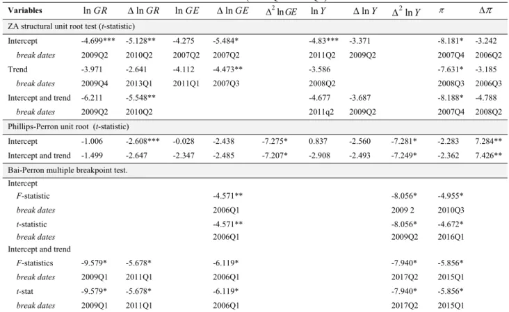
12 rendered the use of conventional unit root tests inappropriate (see, e.g., Zivot and Andrews, 1992; Barnejee et al.1992 and Perron and Vogelsang, 1998 )19. As stated earlier, failure to account for existing endogenous break in a time-series can lead to rejection of the presence of a unit root, which may otherwise be false (see, Perron, 1989; Islam, 2001).
It is, therefore, appropriate to test of unit root against the alternative that data is stationary with breaks in the deterministic trend. For this purpose, we applied the Zivot and Andrews (1992, hereafter ZA) and Phillips-Perron (1997) unit root tests that allow for structural breaks to establish the stationarity properties of each variable as well as identify inherent break dates congruent to existing endogenous breaks in each series. In particular, the ZA-unit root test can confirm the presence of structural breaks in the deterministic trend and also endogenously determine break dates from data, instead of a prior
fixed date (Perron, 1989). We proceed to apply the ZA Model C (same as, Perron and Vogelsang IO Model 2) based on ADF suitable for data with trending data with both intercept and trend breaks. The ZA test is described as:
1 1 k1 1
t t t t t t t t t
y
DU
D
DT
y
y
(13)where
y
t is a time series, indicates the first difference of series, t is a time-trend,k
is the optimal leg length to stationarity ofy
t,
t is the error term.DU
t andDT
t are dummy variables to capture trend shift and men shift respectively, occurring at each possible break date, TB defined as:
1
and
0
0
t tif t >TB
t TB if t >TB
DU
DT
otherwise
otherwise
(14)Whereas, the Phillips-Peron (PP) unit root test is estimated as follows:
t t t t
y
y
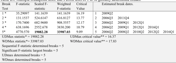
(15)Here, t value is associated with the estimated coefficient of . The series is stationary if is negative and significant. The test is performed both in levels and the first difference of the series to establish stationarity. To abstain from a priori fixed dates, we rely on the break dates identified by three different unit root tests, that is the ZA, PP and Bai-Perron’s multiple breakpoint unit-roots were carried out on each variable, and the results are reported in Table 1. For robustness check, we also perform a multiple breakpoint unit root test on the estimated OLS regression in Eqs. (1) and (2)20, and the results are provided in Tables B1 to B5 in the Appendix.
Possible break dates identified using all the unit root tests for each series are summarised as follows: 2009Q1 and 20011Q2 for government revenues; 2006Q1 and 2006Q2 for government expenditures; 2009Q2 and 2017Q2 for real GDP; and 2010Q3, 2016Q1 and 2015Q2 for inflation. Whereas, the results of the multiple breakpoint tests carried out on the OLS regression in Eqs. (1) and (2) based on sequential breaks, recursive partitions and global crisis induced breaks to show more co-breaking in data, which typically coincide with shocks associated with the global economic and financial crisis, as well as structural endogenous shocks that occurred in the South African economy due to, for example, political uncertainty, fiscal and economic policies. Thus, for parsimony and robustness, dummy variables are constructed to capture the existing breaks in the data.
Because our sample period covers notable structural changes in the South African economy, for example, the inception of the intergovernmental fiscal framework (IGFR) in the post-apartheid era (i.e., 2002) by the National Treasury to effectively manage the distribution of fiscal resources (national
expanding fiscal debt (% of GDP) that is currently above 58% (quote), and (iv) decline in revenue generated since 2017 (Fig.3).
19See, e.g., Perron (2017, 2006) for useful literature on dealing with structural break issue in time-series. 20The OLS equations are estimated in levels (excluding dummies). The multiple breaking point unit root test is
developed based on theoretical contributions of ZA (1992), Baneerjee et al.(1992), Volgesang and Perron (1998) and Perron (1998), among others. This test is carried out in Eviews 10.
13 revenue collected) to sub-national spheres of government; the latest global economic and financial crisis (2007-2012); and the implementation of strict fiscal consolidation strategy since 2013 to curb wasteful spending, rising government expenditure and stimulate economic growth. These significant events and evolution in the South African economy were accounted for by estimating four dummy variables: (i)
full impact of the global economic recession and financial contagion over the period: 2008Q1–2012Q2, (ii) period of a synchronised economic downturn in Africa, from 2009Q1–2011Q421, (iii) sharp fall in
South African economic activity during the period 2009Q1–2010Q4 before recovery at the beginning of 2011, and (iv) the ongoing strict fiscal consolidation period to enforce prudent financial management and good governance for the period 2013Q1–2018Q4. It is worth noting that the constructed dummy variables also capture the identified different break dates by the novel unit root tests applied.
5. Empirical Results and Discussion
We begin our analysis by considering the stationarity properties of the variables. The results of the unit root test unequivocally show that the null hypothesis of unit root with a structural break for most of the time-series variables cannot be rejected at levels, but stationarity is achieved after first differencing. Note, only the inflation series is expected to be stationary in levels, while other variables are I(1) stationary with endogenous structural breaks.
Table 1. Results of structural breaks unit root test (2004Q2–2018Q1)
Variables lnGR lnGR lnGE lnGE 2lnGE lnY lnY 2lnY
ZA structural unit root test (t-statistic)
Intercept -4.699*** -5.128** -4.275 -5.484* -4.83*** -3.371 -8.181* -3.242
break dates 2009Q2 2010Q2 2007Q2 2007Q2 2011Q2 2009Q2 2007Q4 2006Q2
Trend -3.971 -2.641 -4.112 -4.473** -3.586 -7.631* -3.185
break dates 2009Q4 2013Q1 2011Q1 2007Q3 2008Q2 2008Q3 2006Q3
Intercept and trend -6.211 -5.548** -4.677 -3.687 -8.188* -4.788
break dates 2009Q2 2010Q2 2011q2 2009Q2 2007Q4 2008Q2
Phillips-Perron unit root (t-statistic)
Intercept -1.006 -2.608*** -0.028 -2.438 -7.275* 0.837 -2.560 -7.281* -2.283 7.284** Intercept and trend -1.499 -2.647 -2.347 -2.485 -7.207* -2.908 -2.493 -7.249* -2.362 7.426** Bai-Perron multiple breakpoint test.
Intercept
F-statistic -4.571** -8.056* -4.955*
break dates 2006Q1 2009 2 2010Q3
t-statistic -4.571** -8.056* -4.672*
break dates 2006Q1 2009Q2 2016Q1
Intercept and trend
F-statistics -9.579* -5.678* -6.119* -7.940* -5.856*
break dates 2009Q1 2011Q1 2006Q1 2017Q2 2015Q1
t-stat -9.579* -5.678* -6.119* -7.940* -5.856*
break dates 2009Q1 2011Q1 2006Q1 2017Q2 2015Q1
Note: *,**,*** denote 1%, 5% and 10% statistically significance levels, respectively. p-values in ( ) parenthesis.
21The recessionary effect of the global crisis on many African countries including South Africa that begun in 2007
lasted up to 2010, followed by economic recovery in 2011 due to strong demand for commodity export (main component of Africa countries export) from emerging market economies, particularly the BRICs (Brazil, Russia, India, China) group led by China, as well as the adopted counter-fiscal strategy by investing in large infrastructure projects financed with concessional loans from China (IMF, 2009, Arief et al.2010).
14
5.1.Cointegration and Direction of Causality.
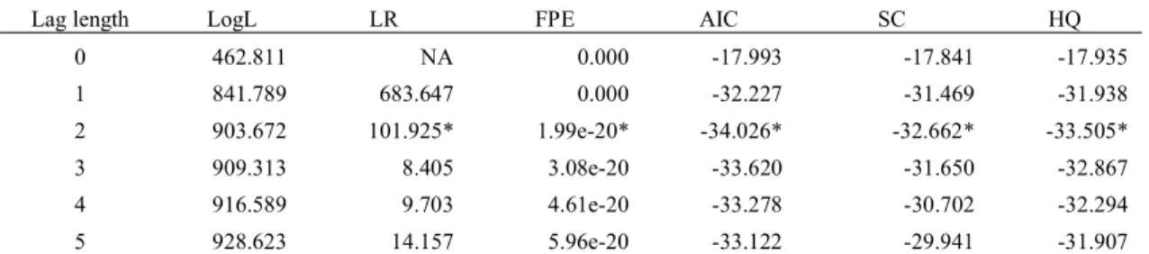
Having confirmed that variables are I(1) stationary, the next step is to examine whether variables are cointegrated, that is, if a long-run relationship exists among variables before assessing the direction of causal links among variables using the vector error correction modelling approach. The Johansen’s (1992,1995) reduced-rank procedure is applied to establish whether variables are linearly cointegrated. The set of information criteria used unanimously to select an optimal lag length of 2, as reported in Table 222, and Table 3 presents the numbers of cointegrating ranks based on the trace and maximum eigenvalue test statistics at 95% significance level. Both test statistics suggest the existence of at least one cointegrated vector (or cointegration equation) between variables at a 5% significance level. Table 2. Optimal lag selection for the cointegration test based on information criteria.
Lag length LogL LR FPE AIC SC HQ
0 462.811 NA 0.000 -17.993 -17.841 -17.935 1 841.789 683.647 0.000 -32.227 -31.469 -31.938 2 903.672 101.925* 1.99e-20* -34.026* -32.662* -33.505* 3 909.313 8.405 3.08e-20 -33.620 -31.650 -32.867 4 916.589 9.703 4.61e-20 -33.278 -30.702 -32.294 5 928.623 14.157 5.96e-20 -33.122 -29.941 -31.907
Note: (*) indicates lag order selected by the criterion. LR, FPE, AIC, SC and HQ denote sequentially modified LR test statistic (each test at 5% level); Final prediction error; Akaike information criterion; Schwarz
information criterion; and Hannan-Quinn information criterion, respectively.
Table 3. Results of VAR-based Johansen unrestricted cointegration rank tests.
H0 H1 Test statistics Critical Values (95%) p-value
Trace Statistics
0
r
r 1 48.555 47.856 0.042 1 r r 2 19.543 29.797 0.454** 2 r r
3
7.305 15.494 0.542Maximum Eigenvalue Statistics
0
r
r 1 29.0114 27.584 0.032 1 r r 2 12.239 21.131 0.524** 2 r r
3
7.216 14.264 0.463Note: p-values based on MacKinnon-Haug-Michelis (1999). *,**,*** denote 1%, 5% and 10% statistically significance levels, respectively.
Since the cointegration test suggests the existence of one linear relationship between the variables in the long run; the error correction models specified Eqs. (9) and (10) were estimated to determine the long-run and temporal causative processes driving the government revenue–expenditure nexus for the Free State province. Before deducing inferences from the models, the dynamic stability estimated error correction models were assessed using the stability test introduced by Brown et al. (1975), and the results are displayed in Figs. B1 and B2 (in the Appendix) which shows that both parameters and variance of the model are dynamically stable under both cumulative sum (CUSUM) and CUSUM of the square tests at a 5% significance level. By implication, obtain results of the estimated error correction models has economic meaning and can be used to draw a robust conclusion on the direction of causal links between variables.
The evidence of long-run relationship existing among variables from the cointegration analysis is validated in the estimated VECMs, and the cointegration equations are represented as:
22The selection criteria are log-likelihood ratio, sequential modified LR test statistic (at 5% significance level),
Final prediction error (FPE), Akaike information criterion (AIC), and Schwarz information criterion (SIC) and Hannan-Quinn (HQ) information.
15 1 1 1 1 ln 0.551 0.419ln 0.019ln 0.004ln [-4.976] [2.222] [2.612] t t t t GR GE Y
(16) 1 1 1 1 ln 3.02 0.94ln 0.11ln 0.02ln [3.472] [7.058] [7.015] t t t t GE GR Y
(17)where, t-stats are in [ ] parenthesis. Note, Eq.(16) shows a positive relationship between government revenue and expenditure, consistent with the tax-spend thesis of Friedman (1978). According to Eq.(16), a one percent increase in the provincial government revenue will raise government expenditure by nearly 0.42% in the long-run and leads to marginal fall in economic activity and inflation by 0.01% and 0.004% respectively. On the contrary, the relationship between government revenue and expenditure in Eq.(17) exhibits an inverse relationship, aligning with Buchanan and Wagner (1977) postulation on the same tax-spend hypothesis. By interpretation, Eq.(17) suggests that a one percent increase in government expenditure exert negative effects on government revenue (-0.94%), economic activity (-0.11%) and inflation (-0.02%). Conclusively, these inferences are economically relevant and robust given the statistically significant t-statistics values at 5% level.
Strikingly, the inferred asymmetric (non-linear) relationship driving the government revenue-expenditure nexus in the Free State province is rather unsurprising. In reference to Ewing et al. (2006), typical asymmetric cointegration between government revenues and expenditures can be attributed to: (i) the differentiated response of the provincial government to either positive or negative changes in fiscal disequilibrium that arises from disproportionate revenue or expenditure levels, (ii) changes in taxpayers behaviour to higher tax rate or tax base, and (iii) the existence of a close link between the business cycle and budget due to the presence of automatic stabilizers, which can cause cyclical fluctuation in budgetary components such as government revenues and expenditures in response to cyclical changes in the business cycle (Ewing et al. 2006:191). The asymmetric relationship between government revenues and expenditures for South Africa has been confirmed in recent studies (see, e.g., Phiri, 2019 and Baharumshah et al. 2016). Elsewhere, see, Saunoris and Payne (2010) and Zapf and Payne (2009) for similar studies.
Next, we turn to the results of the error correction models reported in Table 4. As expected, the error correction terms of both the government revenue equation
F GR GE
(
)
and
F GE GR
(
)
are negative and statistically significant at 5% level, affirming the existence of a stable and long-run relationship among variables in both models. Also, these results suggest a bi-directional long-run causality from government revenue to expenditure and vice-versa, running interactively through real GDP and inflation. This finding suggests the dominance of fiscal synchronicity hypothesis underpins the relationship between government revenue and expenditure in the Free State province, keeping in line with the reported findings by Phiri (2019), Baharumshah et al. (2016), Ghartey (2010), Lusiyan and Thornton (2007) and Nyamongo et al. (2007) for South Africa, but at odds with mixed results documented in earlier cross-sectional studies which support institutional separation or neutrality hypothesis (Narayan and Narayan, 2008) and Spend-Tax hypothesis (Chang, et al.2002) underpinning the causal relationship between revenue and expenditure for South Africa.Additionally, the coefficients of the one-period lagged error correction terms are significantly negative in both dynamic models, but with a varying speed of adjustment to restore fiscal disequilibrium following a shock to the system. Although, the ate of adjustment to restore equilibrium may appear to be relatively slow in both models, nonetheless, fiscal disequilibrium (or imbalance) is corrected by 26% in the
F GR GE
(
)
model compared to a much slower adjustment of about 11% in theF GE GR
(
)
model, in each quarter. The empirical results reveal that the real government expenditure, real GDP and inflation individually Granger causes government revenue in the long-run in the
F GR GE
(
)
model given their statistical significance at 5% level with corresponding significant t-statistics at 1% levels.The result on block causality based on the significant F statistic value (at 5% level) suggests that the independent variables (i.e., real government expenditure, real GDP and inflation rate) jointly
16 Granger causes government revenue in the run. In contrast, there is no evidence supporting long-run causality individually or jointly, from the independent variables to government expenditure in the
( )
F GE GR model.
Table 4. Long-run Granger causality based on the estimated VEC models with dummy variables.
VEC Model 1: GR GE VEC Model 2: GE GR
lnGR p-values lnGE p-values 0
0.0001 [0.508] 0.000*
0 -0.003 [-4.238] 0.000* 2 1 lnECM t -0.256 [-4.125] 0.000* lnECM1 1t -0.107 [-2.991] 0.005* 4 lnGRt -0.2556 [-1.839] 0.039** lnGRt1 -0.331 [-1.870] 0.071*** 1 lnGEt 0.271 [1.995] 0.054** lnGEt1 0.464 [3.229] 0.003* 4 lnYt -0.056 [-2.387] 0.023** lnGEt4 -0.641 [-5.037] 0.000* 3 lnt 0.001 [2.192] 0.036**
1t(xdum01) 0.005 [4.716] 0.000* 5t
(xdum02) 0.001* 0.000*
2t(dd4) 0.005 [6.651] 0.000* 6t
(dd4) 0.000* 0.044**
3t (dfcon) 0.005 [4.142] 0.000* Post-estimation diagnostictests VEC Model 1 VEC Model 2
F-statistic 9.331(0.000)* (0.000)** 14.829 Adjusted
R
2 0.759 0.846 Jarque-Bera 3.975 (0.136) 4.978 (0.082) BG Serial Correlation LM 2.603 (0.272) 2.062 (0.363) ARCH 2.355 (0.124) 0.088 (0.765) Breusch-Pagan-Godfrey 27.695 (0.186) 9.137 (0.995)Note: *,**,*** denotes 1%, 5% and 10% significance levels. 0and 0 denotes constant parameters, p-values for BG LM test, ARCH and BPG test are in ( ) parenthesis with asymptotic values 2 2
*
Obs R .
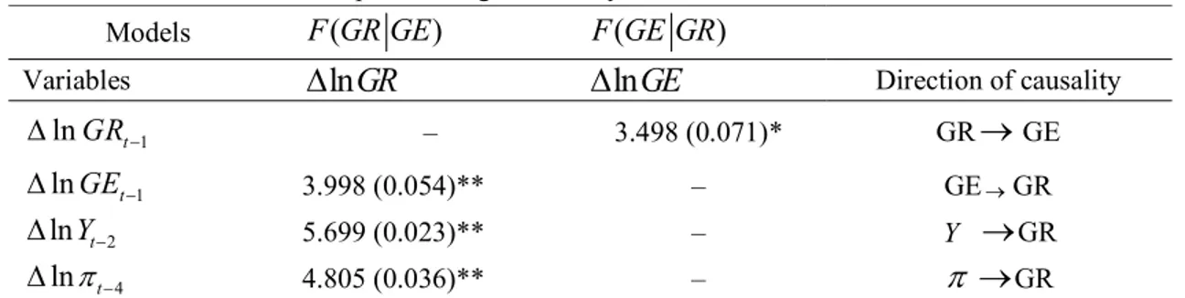
Whereas, the temporal causal link among variables is established in the VECM by applying the standard Fstatistic (or WALD) test, and the results are reported in Table 5. Empirical results show that government revenue Granger causes government expenditure, and vice-versa, suggesting a bi-directional causality in the short run consistent with the fiscal synchronization hypothesis. This result supports the findings of earlier studies that employ advanced econometric techniques such as vector error correction (Nyamongo et al.2007), autoregressive distributed lag (Baharumshah et al.2016, Ghartey, 2010) and momentum threshold autoregressive (Phiri, 2019) models for South Africa. Elsewhere, Owoye et al. (2010) also found short-run fiscal synchronization hypothesis driving the government revenue-expenditure nexus in five European countries, using the ARDL approach during the period 1970 to 2008.
There is also evidence for unidirectional short-run causality from control variables to government revenue in the