Data Stream Classification Using Classifier Ensemble
Micha l Wo´zniak, Andrzej Kasprzak
Department of Systems and Computer Networks, Wroclaw University of Technology, Wyb. Wyspia´nskiego 27, 50-370 Wroc law, Poland
e-mail:[michal.wozniak,andrzej.kasprzak]@pwr.edu.pl
Abstract.For the contemporary business, the crucial factor is making smart decisions on the basis of the knowledge hidden in stored data. Unfortunately, traditional simple methods of data analysis are not sufficient for efficient man-agement of modern enterprizes, because they are not appropriate for the huge and growing amount of the data stored by them. Additionally data usually comes continuously in the form of so-called data stream. The great disadvan-tage of traditional classification methods is that they assume that statistical properties of the discovered concept are being unchanged, while in real sit-uation, we could observe so-called concept drift, which could be caused by changes in the probabilities of classes or/and conditional probability distribu-tions of classes. The potential for considering new training data is an impor-tant feature of machine learning methods used in security applications (spam filtering or intrusion detection) or decision support systems for marketing de-partments, which need to follow the changing client behavior. Unfortunately, the occurrence ofconcept drift dramatically decreases classification accuracy. This work presents the comprehensive study on the ensemble classifier ap-proach applied to the problem of drifted data streams. Especially it reports the research on modifications of previously developed Weighted Aging Classi-fier Ensemble (WAE) algorithm, which is able to construct a valuable classiClassi-fier ensemble for classification of incremental drifted stream data. We general-ize WAE method and propose the general framework for this approach. Such framework can prune an classifier ensemble before or after assigning weights to individual classifiers. Additionally, we propose new classifier pruning criteria, weight calculation methods, and aging operators. We also propose rejuvenat-ing operator, which is able to soften the agrejuvenat-ing effect, which could be useful, especially in the case if quite ”old” classifiers are high quality models, i.e., their presence increases ensemble accuracy, what could be found, e.g., in the case of recurringconcept drift. The chosen characteristics of the proposed frameworks were evaluated on the basis of the wide range of computer experiments carried
out on the two benchmark data streams. Obtained results confirmed the us-ability of proposed method to the data stream classification with the presence of incremental concept drift.
Keywords:data stream classification, classifier enslemble, pattern classifica-tion, forgetting.
1. Introduction
Appearance of concept drift can potentially cause a significant accuracy deterioration of an exploiting classifier.
Therefore, developing positive methods which are able to effectively deal with this phenomena has become an increasing issue in the intense researches. In gen-eral, we can: (i) rebuild a classification model if new data becomes available; (ii) detect concept changes in new data, and if these changes aresufficiently significant then rebuilding the classifier; (iii) adopt an incremental learning algorithm for the classification model. Basically, we can divide these algorithms int: online learners [1], instance based solutions [2], ensemble methods, algorithm based on drift detec-tion [3]. In this work we will focus on the third group consists of algorithms that in-corporate a set of elementary classifiers [4]. The idea of ensemble systems is not new and their effectiveness has been proven in static environments. It has been shown that a collective decision can increase classification accuracy because the knowl-edge that is distributed among the classifiers may be more comprehensive.
2. Data stream classification using classifier ensemble
Let’s concentrate on the problem of using classifier ensemble to data stream classi-fication. It is worth mentioning that in a changing environment diversity can also refer to the context. This makes ensemble systems interesting for researchers dealing with concept drift. Several strategies are possible for a changing environment:
1. Dynamic combiners, where individuals are trained in advance and their rele-vance to the current context is evaluated dynamically while processing subsequent data [5]. The drawback of this approach is that all contexts must be available in advance.
2. Updating the ensemble members, where each ensemble consists of a set of online classifiers that are updated incrementally based on the incoming data [6].
3. Dynamic changing ensemble line-up, e.g., individual classifiers are evaluated dynamically and the worst one is replaced by a new one trained on the most recent data [7].
Among the most popular ensemble approaches, the following are worth noting: the Streaming Ensemble Algorithm (SEA) [8] or the Accuracy Weighted Ensem-ble (AWE) [9]. Both algorithms keep a fixed-size set of classifiers, but the SEA uses a majority voting, whereas the AWE uses the more advanced weighted voting. A similar formula for decision making is implemented in the Dynamic Weighted Majority (DWM) algorithm [10]. Wozniak et al. proposed the dynamic ensemble model called Weighted Aging Ensemble (WAE) [11] which can modify line-up of the classifier committee on the basis of diversity measure. Additionally the decision about object’s label is made according to weighted voting, where weight of a given classifier depends on its accuracy and time spending in an ensemble [11].
3. Weighted Aging Classifier Ensemble
In this section we present the extensions and generalization of the Weighted Aging Classifier Ensemble (WAE) proposed by Wozniak et al. [11]. We will propose several valuable modifications which will be being tested in the future, and new experiments on modified WAE will be presented as well.
WAE is a classifier ensemble method which is able to adapt to the changes in data stream. We assume that the classified data stream is given in a form of data chunks denotes asLSk, wherekis the chunk index. The concept drift could appear
in the incoming data chunks. Instead of drift detection WAE tries to construct self-adapting classifier ensemble. Therefore on the basis of the each chunk one individual is trained and we check if it could form valuable ensemble with the previously trained models. Original WAE uses already presented Generalized Diversity (GD) to choose valuable ensemble and assigns the weights to each individual taking into considera-tion on the one hand frequency of correct classificaconsidera-tion of individual Ψi, denotes as
Pa(Ψi) and on the other hand the number of iterations which Ψi has been spent in
the ensemble -itter(Ψi). This proposition of classifier aging has its root in object
weighting algorithms where an instance weight is usually inversely proportional to the time that has passed since the instance was read [12] and Accuracy Weighted Ensemble (AWE)[9], but the proposed method incudes two important modifications: (i) classifier weights depend on the individual classifier accuracies and how long they have been spending in the ensemble, (ii) individual classifier are chosen to the en-semble on the basis on the non-pairwise diversity measure. Let’s us present the general frameworks of modified WAE called mWAE (modified WAE) (see Alg.1).
Algorithm 1Modified Weighted Aging Ensemble (mWAE) Require: input data stream,
data chunk size,
kclassifier training proceduresT rain1, T rain2, ..., T raink,
ensemble sizeL,
pruning criterioncriterionp,
weight calculatingprocedureweight calc aging procedure,
rejuvenating procedure i:= 1
Π :=∅ repeat
collect new data chunkDSi
forj:= 1to kdo Ψi,j ←T rainj(DSi)
Π := Π∪ {Ψi,j} to the classifier ensemble Π
end for
w(Ψj)←rejuvenating(Π,Ψj)
if |Π|> Lthen
choose the most valuable ensemble ofLclassifiers usingcriterionp
end if w:= 0 forj:= 1to |Π|do w(Ψj)←weight calculating(Π,Ψj, DSi) w(Ψj)←aging(Ψj) if w(Ψj) == 0then Π = Π\{Ψj} end if w:=w+w(Ψj) end for forj:= 1to |Π|do w(Ψj) :=w(Ψwj) end for i:=i+ 1
untilend of the input data stream
3.1. Pruning criterion
We propose to use weighted combination of diversity measure and ensemble accuracy. criterion(Π) =αPaensemble(Π) + (1−α)diversity(Π) (1)
wherediversity(Π) stands for diversity measure value of Π andalpha∈[0,1] is user defined value – smallαpromotes accuracy, whileαclose to 1 boosts the impact of diversity. The remark about used accuracy is the same as previously.
3.2. Weight calculation
We propose the following methods of weight calculation: The same weights for each classifierin the pool, i.e., majority vote is use as the combination rule
w(Ψi) =
1
|Π| (2)
Weights proportional to classifier accuracy
w(Ψi) =Pa(Ψi) (3)
Aged weights proportional to classifier accuracyused by the original WAE algorithm [13] w(Ψi) = Pa(Ψi) p itter(Ψi) (4) This weight calculation includes aging as well (i.e., forgetting).
Kuncheva’s weights– suggested by Kuncheva in her book [14] w(Ψi) = Pa(Ψi)
1−Pa(Ψi)
(5)
3.3. Aging
We propose the following aging methods:
Aged weights proportional to classifier accuracy used by the original WAE algorithm [13] and presented in the previous section.
w(Ψi) =
Pa(Ψi)
p
itter(Ψi)
(6) It was described in the previous section.
Constant aging w(Ψi) =
(
w(Ψi) =w(Ψi)−δ ifw(Ψi) =w(Ψi)−δ > θ
0 otherwise (7)
where theta ∈ [0,1] as previously stands for the parameter responsible for the re-moving less important (old enough) classifiers.
Gaussian aging w(Ψi) = 1 2πexp itter(Ψi)ξ 2 if 1 2πexp itter(Ψi)ξ 2 > θ 0 otherwise (8)
whereθ∈[0,1] as previously stands for the parameter responsible for the removing less important (old enough) classifiers andxiis used defined parameter.
3.4. Rejuvenating
We propose to rejuvenate an individual classifier if it has a big impact on the classifier ensemble accuracy. This could be useful especially in the case of recurring concept drift. The idea is presented in Alg. 2, where [] stands forentier.
Algorithm 2Rejuvenating
Require: power of rejuvenatingrejun pow
weights {w(Ψ1), w(Ψ2)...} assigned to the individuals in Π 1: w:= 0 2: forj:= 1 to|Π| do 3: w:=w+w(Ψj) 4: end for 5: forj:= 1 to|Π| do 6: if w(Ψj)> wthen
7: itter(Ψj) :=itter(Ψj)−[rejunpow(w(Ψj)−w)]
8: end if 9: end for
4. Experimental Investigations
The presented experiments had preliminary nature and their results would be a start-ing point for future research on WAE inspired algorithms. The aims of the experi-ment were assessing if the proposed method of weighting and aging individual clas-sifiers in the ensemble is valuable proposition compared with the methods which do not include aging or weighting techniques, and establishing the dependency between theαin combined pruning criterion (eq. 1) and quality of the proposed algorithm.
4.1. Set-up
All experiments were carried out on two syntectic benchmark datasets:
• The SEA dataset [8], where we simulated drift by instant random model change (it was observed in objects no. 415, 971, 1525, 2194).
• Hyper Plane Stream [15] where each object belongs to one of the 5 classes and is described by 10 attributes. The dataset is a synthetic data stream containing gradually evolving (drifting) concepts. The drift is appeared each 800 observations.
For the experiments we decided to form heterogenous ensemble, i.e., ensemble which consists of the classifiers using the different models (to ensure its higher di-versity). We used the following models for individual classifiers:
• Na¨ıve Bayes,
• decision tree trained by C4.5 [16],
• SVM with polynomial kernel trained by the sequential minimal optimization method (SMO) [17],
• nearest neighbor classifier,
• classifier using a multinominal logistic regression with a ridge classier [18], • OneR [19].
During each of the experiment we tried to evaluate dependency between data chunk sizes (which were fixed on 50, 100, 150, 200) and overall classifier quality (accuracy and standard deviation) and the diversity of the best ensemble for the following ensembles:
1. simple – an ensemble using majority voting without aging.
2. weighted – an ensemble using weighted voting without aging, where weight assigned to a given classifier is inversely proportional to its accuracy.
3. weighted aged – an ensemble using weighted voting with aging, where weight assigned to a given classifier is calculated according to eq.1.
All experiments were carried out in the Java environment using Weka classi-fiers [20].
The new individual classifiers were trained on a given data chunk. The same chunk was used to prune the classifier committee, but the ensemble error was esti-mated on the basis on the next (unseen) portion of data.
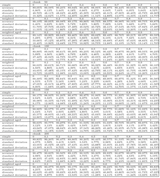
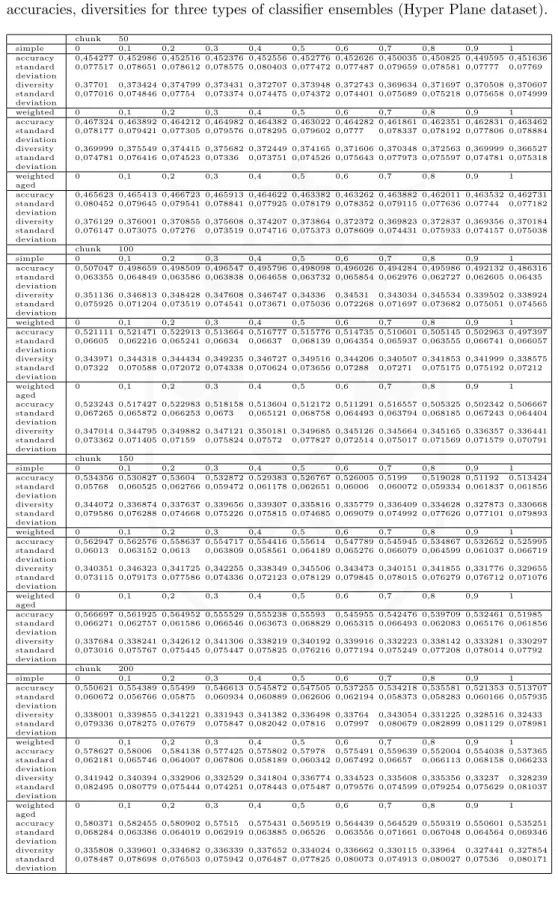
The experiments were run for differentαvalues (α∈ {0.0,0.2, ...,1.0}) and their results are presented in Tab. 1–2.
Tab. 1. Dependencies betweenαvalue used in the pruning criterion and ensembles’ accuracies, diversities for three types of classifier ensembles (SEA dataset).
chunk 50 simple 0 0,1 0,2 0,3 0,4 0,5 0,6 0,7 0,8 0,9 1 accuracy 89,05% 89,59% 90,25% 89,94% 89,46% 88,95% 89,97% 88,44% 89,65% 90,32% 89,02% standard deviation 6,90% 6,13% 5,44% 6,18% 6,66% 6,27% 6,04% 7,03% 6,05% 5,64% 6,52% diversity 49,70% 48,11% 48,02% 46,42% 45,39% 50,90% 46,31% 47,96% 46,43% 45,73% 48,96% standard deviation 10,42% 12,62% 11,57% 12,40% 12,38% 11,52% 12,89% 13,07% 14,33% 12,64% 13,75% weighted 0 0,1 0,2 0,3 0,4 0,5 0,6 0,7 0,8 0,9 1 accuracy 88,10% 89,05% 89,08% 89,17% 89,90% 89,75% 88,57% 88,98% 90,16% 89,75% 89,87% standard deviation 6,40% 6,62% 6,38% 5,72% 5,85% 5,80% 7,06% 6,53% 5,68% 6,07% 5,82% diversity 51,70% 47,70% 49,34% 47,48% 46,02% 49,72% 46,11% 47,54% 48,73% 47,82% 47,48% standard deviation 11,55% 12,10% 11,80% 12,30% 13,07% 12,45% 12,03% 12,58% 12,20% 11,44% 12,55% weighted aged 0 0,1 0,2 0,3 0,4 0,5 0,6 0,7 0,8 0,9 1 accuracy 89,14% 89,90% 89,94% 89,46% 90,32% 89,02% 89,49% 88,76% 89,21% 89,97% 89,59% standard deviation 5,28% 5,97% 5,95% 6,31% 5,66% 6,50% 6,10% 6,31% 7,32% 6,04% 6,10% diversity 50,66% 47,12% 46,87% 47,28% 47,88% 48,54% 49,68% 47,83% 47,63% 48,83% 45,77% standard deviation 10,49% 10,90% 12,44% 12,77% 10,92% 10,75% 12,88% 12,19% 13,76% 13,14% 11,70% chunk 100 simple 0 0,1 0,2 0,3 0,4 0,5 0,6 0,7 0,8 0,9 1 accuracy 89,90% 89,94% 90,61% 90,39% 89,23% 90,52% 90,42% 90,87% 90,26% 89,55% 90,23% standard deviation 5,09% 4,56% 4,28% 4,79% 4,89% 4,46% 4,28% 4,63% 4,91% 5,07% 4,70% diversity 47,42% 46,94% 44,79% 50,07% 47,16% 49,05% 48,27% 43,80% 43,55% 46,00% 45,34% standard deviation 11,10% 13,10% 10,77% 8,46% 9,81% 13,62% 11,24% 11,22% 13,39% 12,71% 12,32% weighted 0 0,1 0,2 0,3 0,4 0,5 0,6 0,7 0,8 0,9 1 accuracy 90,03% 90,61% 90,71% 90,68% 88,87% 90,32% 90,48% 90,55% 91,32% 91,00% 90,10% standard deviation 4,56% 4,86% 4,34% 4,39% 5,66% 5,21% 4,65% 4,65% 3,65% 4,70% 4,13% diversity 44,65% 47,48% 45,15% 47,42% 46,02% 43,79% 46,11% 44,42% 41,73% 44,08% 43,96% standard deviation 12,72% 10,05% 11,98% 10,02% 13,09% 12,43% 10,55% 10,24% 16,17% 10,20% 12,61% weighted aged 0 0,1 0,2 0,3 0,4 0,5 0,6 0,7 0,8 0,9 1 accuracy 90,39% 90,39% 89,84% 90,84% 90,19% 90,19% 89,90% 90,97% 91,32% 91,48% 90,58% standard deviation 4,55% 4,71% 5,16% 3,99% 5,23% 5,23% 4,00% 4,29% 4,50% 4,00% 4,19% diversity 47,05% 45,91% 44,87% 47,89% 45,09% 47,77% 46,26% 44,11% 43,95% 47,53% 41,58% standard deviation 9,90% 11,68% 10,46% 10,49% 13,49% 11,12% 10,47% 12,70% 11,57% 11,54% 8,97% chunk 150 simple 0 0,1 0,2 0,3 0,4 0,5 0,6 0,7 0,8 0,9 1 accuracy 90,17% 88,93% 91,20% 90,47% 90,47% 91,00% 90,77% 91,33% 91,30% 91,60% 90,23% standard deviation 2,94% 3,32% 3,45% 3,88% 3,37% 3,54% 3,80% 3,57% 3,28% 3,73% 3,91% diversity 46,98% 44,33% 42,74% 41,49% 41,72% 44,21% 45,06% 43,51% 44,31% 42,09% 44,23% standard deviation 9,17% 12,90% 14,08% 12,43% 11,24% 14,23% 11,15% 16,00% 11,18% 11,67% 10,33% weighted 0 0,1 0,2 0,3 0,4 0,5 0,6 0,7 0,8 0,9 1 accuracy 90,90% 90,57% 91,47% 90,37% 90,80% 90,87% 90,77% 91,00% 91,10% 91,03% 91,80% standard deviation 3,44% 3,74% 2,93% 4,06% 4,80% 3,19% 3,01% 3,58% 4,05% 3,55% 3,70% diversity 45,57% 48,83% 43,14% 49,22% 43,56% 45,69% 38,68% 42,04% 43,63% 46,88% 45,94% standard deviation 12,86% 13,87% 14,20% 13,33% 14,54% 9,18% 15,18% 15,10% 11,68% 8,01% 8,83% weighted aged 0 0,1 0,2 0,3 0,4 0,5 0,6 0,7 0,8 0,9 1 accuracy 90,63% 90,77% 90,27% 91,33% 91,53% 90,83% 91,03% 90,70% 90,67% 89,87% 91,13% standard deviation 3,12% 3,13% 3,42% 3,42% 3,59% 3,23% 3,81% 3,52% 3,11% 2,97% 3,42% diversity 43,04% 47,07% 48,04% 45,56% 37,54% 46,20% 45,46% 45,95% 45,71% 45,28% 41,39% standard deviation 13,08% 14,18% 9,04% 14,08% 14,79% 10,23% 10,72% 9,70% 9,52% 39,04% 13,17% chunk 200 simple 0 0,1 0,2 0,3 0,4 0,5 0,6 0,7 0,8 0,9 1 accuracy 89,83% 90,20% 90,47% 89,90% 90,20% 90,43% 90,57% 91,53% 90,20% 90,73% 90,53% standard deviation 4,37% 3,59% 3,41% 3,56% 3,53% 3,77% 2,98% 2,82% 3,37% 3,58% 3,49% diversity 43,05% 45,02% 48,42% 47,43% 44,00% 43,88% 45,05% 43,44% 47,78% 50,06% 46,40% standard deviation 13,39% 8,91% 9,75% 9,79% 15,04% 10,82% 14,91% 9,01% 7,20% 6,96% 14,73% weighted 0 0,1 0,2 0,3 0,4 0,5 0,6 0,7 0,8 0,9 1 accuracy 90,47% 90,83% 90,50% 89,13% 90,53% 90,30% 89,93% 90,67% 89,87% 89,97% 86,93% standard deviation 2,98% 2,94% 3,08% 4,42% 3,76% 3,47% 3,78% 3,22% 4,53% 2,97% 5,19% diversity 48,23% 47,43% 42,83% 51,08% 45,29% 43,56% 45,34% 41,74% 47,84% 44,65% 38,13% standard deviation 8,82% 7,95% 13,88% 6,36% 12,22% 9,96% 8,77% 10,23% 12,89% 11,85% 12,77% weighted aged 0 0,1 0,2 0,3 0,4 0,5 0,6 0,7 0,8 0,9 1 accuracy 90,43% 90,37% 90,80% 90,17% 90,53% 90,20% 90,23% 90,70% 90,53% 90,20% 89,83% standard deviation 4,25% 4,04% 3,57% 3,67% 3,40% 4,13% 3,07% 2,96% 3,88% 3,78% 4,05% diversity 46,62% 43,49% 39,69% 42,84% 38,59% 42,26% 40,80% 43,86% 44,54% 41,73% 47,22% standard deviation 10,12% 9,87% 9,95% 13,53% 11,12% 11,28% 14,11% 9,97% 11,44% 13,93% 8,99%
Tab. 2. Dependencies betweenαvalue used in the pruning criterion and ensembles’ accuracies, diversities for three types of classifier ensembles (Hyper Plane dataset).
chunk 50 simple 0 0,1 0,2 0,3 0,4 0,5 0,6 0,7 0,8 0,9 1 accuracy 0,454277 0,452986 0,452516 0,452376 0,452556 0,452776 0,452626 0,450035 0,450825 0,449595 0,451636 standard deviation 0,077517 0,078651 0,078612 0,078575 0,080403 0,077472 0,077487 0,079659 0,078581 0,07777 0,07769 diversity 0,37701 0,373424 0,374799 0,373431 0,372707 0,373948 0,372743 0,369634 0,371697 0,370508 0,370607 standard deviation 0,077016 0,074846 0,07754 0,073374 0,074475 0,074372 0,074401 0,075689 0,075218 0,075658 0,074999 weighted 0 0,1 0,2 0,3 0,4 0,5 0,6 0,7 0,8 0,9 1 accuracy 0,467324 0,463892 0,464212 0,464982 0,464382 0,463022 0,464282 0,461861 0,462351 0,462831 0,463462 standard deviation 0,078177 0,079421 0,077305 0,079576 0,078295 0,079602 0,0777 0,078337 0,078192 0,077806 0,078884 diversity 0,369999 0,375549 0,374415 0,375682 0,372449 0,374165 0,371606 0,370348 0,372563 0,369999 0,366527 standard deviation 0,074781 0,076416 0,074523 0,07336 0,073751 0,074526 0,075643 0,077973 0,075597 0,074781 0,075318 weighted aged 0 0,1 0,2 0,3 0,4 0,5 0,6 0,7 0,8 0,9 1 accuracy 0,465623 0,465413 0,466723 0,465913 0,464622 0,463382 0,463262 0,463882 0,462011 0,463532 0,462731 standard deviation 0,080452 0,079645 0,079541 0,078841 0,077925 0,078179 0,078352 0,079115 0,077636 0,07744 0,077182 diversity 0,376129 0,376001 0,370855 0,375608 0,374207 0,373864 0,372372 0,369823 0,372837 0,369356 0,370184 standard deviation 0,076147 0,073075 0,07276 0,073519 0,074716 0,075373 0,078609 0,074431 0,075933 0,074157 0,075038 chunk 100 simple 0 0,1 0,2 0,3 0,4 0,5 0,6 0,7 0,8 0,9 1 accuracy 0,507047 0,498659 0,498509 0,496547 0,495796 0,498098 0,496026 0,494284 0,495986 0,492132 0,486316 standard deviation 0,063355 0,064849 0,063586 0,063838 0,064658 0,063732 0,065854 0,062976 0,062727 0,062605 0,06435 diversity 0,351136 0,346813 0,348428 0,347608 0,346747 0,34336 0,34531 0,343034 0,345534 0,339502 0,338924 standard deviation 0,075925 0,071204 0,073519 0,074541 0,073671 0,075036 0,072268 0,071697 0,073682 0,075051 0,074565 weighted 0 0,1 0,2 0,3 0,4 0,5 0,6 0,7 0,8 0,9 1 accuracy 0,521111 0,521471 0,522913 0,513664 0,516777 0,515776 0,514735 0,510601 0,505145 0,502963 0,497397 standard deviation 0,06605 0,062216 0,065241 0,06634 0,06637 0,068139 0,064354 0,065937 0,063555 0,066741 0,066057 diversity 0,343971 0,344318 0,344434 0,349235 0,346727 0,349516 0,344206 0,340507 0,341853 0,341999 0,338575 standard deviation 0,07322 0,070588 0,072072 0,074338 0,070624 0,073656 0,07288 0,07271 0,075175 0,075192 0,07212 weighted aged 0 0,1 0,2 0,3 0,4 0,5 0,6 0,7 0,8 0,9 1 accuracy 0,523243 0,517427 0,522983 0,518158 0,513604 0,512172 0,511291 0,516557 0,505325 0,502342 0,506667 standard deviation 0,067265 0,065872 0,066253 0,0673 0,065121 0,068758 0,064493 0,063794 0,068185 0,067243 0,064404 diversity 0,347014 0,344795 0,349882 0,347121 0,350181 0,349685 0,345126 0,345664 0,345165 0,336357 0,336441 standard deviation 0,073362 0,071405 0,07159 0,075824 0,07572 0,077827 0,072514 0,075017 0,071569 0,071579 0,070791 chunk 150 simple 0 0,1 0,2 0,3 0,4 0,5 0,6 0,7 0,8 0,9 1 accuracy 0,534356 0,530827 0,53604 0,532872 0,529383 0,526767 0,526005 0,5199 0,519028 0,51192 0,513424 standard deviation 0,05768 0,060525 0,062766 0,059472 0,061178 0,062651 0,06006 0,060072 0,059334 0,061837 0,061856 diversity 0,344072 0,336874 0,337637 0,339656 0,339307 0,335816 0,335779 0,336409 0,334628 0,327873 0,330668 standard deviation 0,079586 0,076288 0,074668 0,075226 0,075815 0,074685 0,069079 0,074992 0,077626 0,077101 0,079893 weighted 0 0,1 0,2 0,3 0,4 0,5 0,6 0,7 0,8 0,9 1 accuracy 0,562947 0,562576 0,558637 0,554717 0,554416 0,55614 0,547789 0,545945 0,534867 0,532652 0,525995 standard deviation 0,06013 0,063152 0,0613 0,063809 0,058561 0,064189 0,065276 0,066079 0,064599 0,061037 0,066719 diversity 0,340351 0,346323 0,341725 0,342255 0,338349 0,345506 0,343473 0,340151 0,341855 0,331776 0,329655 standard deviation 0,073115 0,079173 0,077586 0,074336 0,072123 0,078129 0,079845 0,078015 0,076279 0,076712 0,071076 weighted aged 0 0,1 0,2 0,3 0,4 0,5 0,6 0,7 0,8 0,9 1 accuracy 0,566697 0,561925 0,564952 0,555529 0,555238 0,55593 0,545955 0,542476 0,539709 0,532461 0,51985 standard deviation 0,066271 0,062757 0,061586 0,066546 0,063673 0,068829 0,065315 0,066493 0,062083 0,065176 0,061856 diversity 0,337684 0,338241 0,342612 0,341306 0,338219 0,340192 0,339916 0,332223 0,338142 0,333281 0,330297 standard deviation 0,073016 0,075767 0,075445 0,075447 0,075825 0,076216 0,077194 0,075249 0,077208 0,078014 0,07792 chunk 200 simple 0 0,1 0,2 0,3 0,4 0,5 0,6 0,7 0,8 0,9 1 accuracy 0,550621 0,554389 0,55499 0,546613 0,545872 0,547505 0,537255 0,534218 0,535581 0,521353 0,513707 standard deviation 0,060672 0,056766 0,05875 0,060934 0,060889 0,062606 0,062194 0,058373 0,058283 0,060166 0,057935 diversity 0,338001 0,339855 0,341221 0,331943 0,341382 0,336498 0,33764 0,343054 0,331225 0,328516 0,32433 standard deviation 0,079336 0,078275 0,07679 0,075847 0,082042 0,07816 0,07997 0,080679 0,082899 0,081129 0,078981 weighted 0 0,1 0,2 0,3 0,4 0,5 0,6 0,7 0,8 0,9 1 accuracy 0,578627 0,58006 0,584138 0,577425 0,575802 0,57978 0,575491 0,559639 0,552004 0,554038 0,537365 standard deviation 0,062181 0,065746 0,064007 0,067806 0,058189 0,060342 0,067492 0,06657 0,066113 0,068158 0,066233 diversity 0,341942 0,340394 0,332906 0,332529 0,341804 0,336774 0,334523 0,335608 0,335356 0,33237 0,328239 standard deviation 0,082495 0,080779 0,075444 0,074251 0,078443 0,075487 0,079576 0,074599 0,079254 0,075629 0,081037 weighted aged 0 0,1 0,2 0,3 0,4 0,5 0,6 0,7 0,8 0,9 1 accuracy 0,580371 0,582455 0,580902 0,57515 0,575431 0,569519 0,564439 0,564529 0,559319 0,550601 0,535251 standard deviation 0,068284 0,063386 0,064019 0,062919 0,063885 0,06526 0,063556 0,071661 0,067048 0,064564 0,069346 diversity 0,335808 0,339601 0,334682 0,336339 0,337652 0,334024 0,336662 0,330115 0,33964 0,327441 0,327854 standard deviation 0,078487 0,078698 0,076503 0,075942 0,076487 0,077825 0,080073 0,074913 0,080027 0,07536 0,080171
4.2. Results discussion
We realize that the scope of the experiments we carried out is limited and derived remarks are limited to the tested methods and one dataset only. In this case for-mulating general conclusions is very risky, but the preliminary results are quite promising, therefore we would like to continue the work on WAE inspired methods in the future. Let’s focus on some interesting observations:
• The experiments confirmed that proposed approach can adapt to changing concept returning a quite stable classifier. According to the obtained results we can confirm that for this model the heterogenous ensemble is the best model, especially if it bases on accuracy criterion only (i.e.,α= 1 in criterion given by eq. 1), because it is clearly visible that using the diversity measure as the pruning criterion is not appropriate for the data stream classification task.
• The standard deviation is smaller for bigger data chunk and usually standard deviation of WAE inspired method is smallest among all tested methods. It means that the concept drift appearances have the weakest impact on the accuracy of WAE inspired methods.
• The overall accuracies of the tested ensembles are stable according to the chunk sizes for SEA dataset. The standard deviation of the accuracies is unstable, but it is smallest for the chunk size 150. The observation is useful because the bigger size of data chunk means that effort dedicated to building new models is smaller because they are being built rarely.
• The interesting observation may be made analyzing the dependency among α factor values, diversity, and accuracy of the ensembles. The clear tenden-cies were observed for Hyper Plane Stream dataset only. The accuracy and diversity were decreasing according to the α value. It is surprising, because if α is close to 1 then the diversity should play the key role in the pruning criterion, but the overall diversity is higher for the ensembles formed using the mentioned criterion for the small α(what means that accuracy plays the key role in this criterion).
• Another interesting observation is that the standard deviation is smaller for bigger data chunk and usually standard deviation of WAE inspired algorithm is smallest among all tested methods. It means that the concept drift appear-ances have the weakest impact on the accuracy of the WAE inspired methods.
5. Conclusions
We have to notice the limitation of considered approach. Both the proposed ensem-ble does not use more sophisticated combination method based on support functions.
For the heterogenous ensemble it is mostly impossible, but homogenous ensemble could be used, or at least ensemble of classifiers which produce the same type of sup-port functions. Therefore we would like to emphasize that we presented preliminary study on WAE inspired methods which is a starting point for the future research. Used diversity measure does not seem to be appropriate for the data stream classi-fication tasks, therefore we would like to extend the scope of experiments by using another non-pairwise diversity measures and maybe to propose a new one which can evaluate diversity taking into consideration the nature of the discussed pattern classification task.
We realize that the scope of the experiments we carried out is limited and de-rived remarks are limited to the tested methods and one dataset only. In this case formulating general conclusions is very risky, but the preliminary results are quite promising, therefore we would like to continue the work on WAE inspired methods in the future. Additionally, it is worth noting that classifier ensemble is a promising research direction for aforementioned problem, but its combination with a drift de-tection algorithm could have a higher impact to the classification performance.
This work was supported by the Polish National Science Centre under the grant no. DEC-2013/09/B/ST6/02264.
6. References
[1] Domingos P., Hulten G.,A general framework for mining massive data streams,
Journal of Computational and Graphical Statistics 12, 2003, pp. 945–949. [2] Widmer G., Kubat M., Learning in the presence of concept drift and hidden
contexts,Mach. Learn. 23 (1), Apr. 1996, pp. 69–101.
[3] Kifer D., Ben-David S., Gehrke J.,Detecting change in data streams, Proceed-ings of the Thirtieth international conference on Very large data bases - Vol. 30, ser. VLDB ’04. VLDB Endowment, 2004, pp. 180–191.
[4] Tsymbal A., Pechenizkiy M., Cunningham P., Puuronen S., Dynamic inte-gration of classifiers for handling concept drift, Inf. Fusion 9 (1), Jan. 2008, pp. 56–68.
[5] Littlestone N., Warmuth M.K.,The weighted majority algorithm,Inf. Comput. 108 (2), Feb. 1994, pp. 212–261.
[6] Bifet A., Holmes G., Pfahringer B., Read J., Kranen P., Kremer H., Jansen T., Seidl T., Moa: A real-time analytics open source framework, Proc. European Conference on Machine Learning and Principles and Practice of Knowledge Dis-covery in Databases (ECML PKDD 2011), Athens, Greece, Springer Heidelberg, Germany, 2011, pp. 617–620.
[7] Jackowski K., Fixed-size ensemble classifier system evolutionarily adapted to a recurring context with an unlimited pool of classifiers, Pattern Analysis and Applications, 2013, pp. 1–16.
[8] Street W.N., Kim Y.,A streaming ensemble algorithm (sea) for large-scale clas-sification,Proceedings of the seventh ACM SIGKDD international conference on Knowledge discovery and data mining, ser. KDD ’01 ACM. New York, NY, USA, 2001, pp. 377–382.
[9] Wang H., Fan W., Yu P.S., Han J., Mining concept-drifting data streams us-ing ensemble classifiers,Proceedings of the ninth ACM SIGKDD international conference on Knowledge discovery and data mining, ser. KDD ’03 ACM. New York, NY, USA, 2003, pp. 226–235.
[10] Kolter J., Maloof M.,Dynamic weighted majority: A new ensemble method for tracking concept drift,in Data Mining, 2003. ICDM 2003. Third IEEE Interna-tional Conference on, Nov. 2003, pp. 123 – 130.
[11] Wozniak M., Kasprzak A., Cal P., Application of combined classifiers to data stream classification,Proceedings of the 10th International Conference on Flex-ible Query Answering Systems FQAS 2013, ser. LNCS Springer-Verlag. Berlin– Heidelberg, 2013, in press.
[12] Klinkenberg R., Renz I., Adaptive information filtering: Learning in the pres-ence of concept drifts,AAAI Technical Report WS-98-05, 1998, pp. 33–40. [13] Wozniak M., Hybrid Classifiers – Methods of Data, Knowledge, and Classifier
Combination, ser. Studies in Computational Intelligence, Springer 519, 2014. [14] Kuncheva L.I., Combining Pattern Classifiers: Methods and Algorithms,
Wiley-Interscience, Hoboken, New Jersey, USA, 2004.
[15] X.X.,Stream data mining repository, http://www.cse.fau.edu/˜xqzhu/stream. html, 2010.
[16] Quinlan J., C4.5: Programs for Machine Learning, ser. Morgan Kaufmann Series in Machine Learning. Morgan Kaufmann Publishers, London, Eng-land, 1993.
[17] Platt J.C.,Advances in kernel methods,B. Sch¨olkopf, C.J.C. Burges, A.J. Smola (Eds.) MIT Press Cambridge, MA, USA, 1999, ch. Fast training of support vector machines using sequential minimal optimization, pp. 185–208.
[18] Le Cessie S., Van Houwelingen J.,Ridge estimators in logistic regression, Ap-plied statistics, 1992, pp. 191–201.
[19] Holte R.C., Very simple classification rules perform well on most commonly used datasets,Machine Learning 11, 1993, pp. 63–91.
[20] Hall M., Frank E., Holmes G., Pfahringer B., Reutemann P., Witten I.H.,
The Weka data mining software: An update, SIGKDD Explor. Newsl. 11 (1), Nov. 2009, pp. 10–18.