This is the post peer-review accepted manuscript of:
A. Burrello, L. Cavigelli, K. Schindler, L. Benini and A. Rahimi, "Laelaps: An
Energy-Efficient Seizure Detection Algorithm from Long-term Human iEEG Recordings
without False Alarms," 2019 Design, Automation & Test in Europe Conference &
Exhibition (DATE), Florence, Italy, 2019, pp. 752-757.
The published version is available online at:
https://ieeexplore.ieee.org/document/8715186
© 2019 IEEE. Personal use of this material is permitted. Permission from IEEE must be obtained for all other
uses, in any current or future media, including reprinting/republishing this material for advertising or
promotional purposes, creating new collective works, for resale or redistribution to servers or lists, or reuse
of any copyrighted component of this work in other works.
Laelaps: An Energy-Efficient Seizure Detection
Algorithm from Long-term Human iEEG Recordings
without False Alarms
Alessio Burrello
∗, Lukas Cavigelli
∗, Kaspar Schindler
†, Luca Benini
∗, Abbas Rahimi
∗∗Integrated Systems Laboratory, ETH Zurich, Switzerland†Sleep-Wake-Epilepsy-Center, Inselspital Bern, Switzerland
Emails: [email protected], [email protected],{cavigelli, benini, abbas}@iis.ee.ethz.ch
Abstract—We propose Laelaps, an energy-efficient and fast learn-ing algorithm with no false alarms for epileptic seizure detection from long-term intracranial electroencephalography (iEEG) signals. Laelaps uses end-to-end binary operations by exploiting symbolic dynamics and brain-inspired hyperdimensional computing. Laelaps’s results surpass those yielded by state-of-the-art (SoA) methods [1], [2], [3], including deep learning, on a new very large dataset containing 116 seizures of 18 drug-resistant epilepsy patients in 2656 hours of recordings—each patient implanted with 24 to 128 iEEG electrodes. Laelaps trains 18 patient-specific models by using only 24 seizures: 12 models are trained with one seizure per patient, the others with two seizures. The trained models detect 79 out of 92
unseen seizureswithout any false alarms across all the patientsas a
big step forward in practical seizure detection. Importantly, a simple implementation of Laelaps on the Nvidia Tegra X2 embedded device
achieves 1.7×–3.9× faster execution and 1.4×–2.9× lower energy
consumption compared to the best result from the SoA methods. Our source code and anonymized iEEG dataset are freely available at http://ieeg-swez.ethz.ch.
Index Terms—Hyperdimensional computing, symbolic analysis.
I. INTRODUCTION
Epilepsy is a highly prevalent chronic neurological disorder affecting 1–2% of the world’s population [4]. One third of patients with epilepsy continue to suffer from seizures despite pharmaco-logical therapy. For improved monitoring of these patients with drug-resistant epilepsy—e.g., during presurgical diagnostics— machine learning methods are developed for automatic seizure detection. These SoA methods are based on extracting useful features followed by traditional supervised machine learning methods such as K-nearest neighbor [5], random forest [6], [4], and support vector machines (SVMs) [1], [7]; more recent methods exploit automatic feature extraction algorithms based on deep learning such as convolutional neural networks (CNNs) [2] and long short-term memories (LSTMs) [3].
Most seizure detection methods assume that the patients with epilepsy experience two distinct states of brain activity—i.e., interictal (between seizures) and ictal (during seizures)—that can be detected by EEG. Recent methods propose to use unobtru-sive non-EEG signals such as heart rate and accelerometry that despite the distance from the seizure generating brain regions reflect extracerebral changes associated with specific types of seizures [8]. However, these methods suffer from high false alarm rates as high as 1.2 h−1 [9], compared to lower (e.g.,
0.47 h−1 [5] to 0.27 h−1 [7]) yielded by EEG-based methods; the false alarms may increase anxiety in epilepsy patients and are thus likely to further decrease their already impaired quality of life [10]. Enabling even more proximate monitoring of the seizure generating regions, intracranial EEG (iEEG, or ECoG) currently
provides the best spatial resolution and highest signal-to-noise ratio to record electrical brain activity [4]. Using such invasive recordings can reduce the false alarm rate to0.13 h−1[11].
However, one major challenge with iEEG signals is to real-ize seizure detection algorithms with low complexity suitable for execution on implantable devices with limited battery size for long-term or even lifelong operation. Another challenge— common to all methods—is to reliably detect seizures from a small number of examples due to the uneven distribution with much longer interictal than ictal time periods, and the patient-specific seizure dynamics [7], [12]. To address these challenges, one promising option is to develop computationally efficient and fast learning algorithms by combining methods from symbolic dynamics [5], [13], [14], [15], [1] and brain-inspired hyperdi-mensional computing [16], [17]. In this paper, we describe the following contributions:
(1) We propose Laelaps1, an energy-efficient algorithm for both
learning and inference from long-term iEEG recording of patients having large heterogeneity implanted with 24 to 128 electrodes. Laelaps operates with end-to-end binary operations to avoid otherwise expensive fixed- or floating-point arithmetic. Laelaps exploits local binary patterns (Sec. II-A) to map a sequence of iEEG samples into 6-bit codes as abstract symbols. These symbols are further combined over time and across all the electrodes to generate a compact representation for encoding the brain state of interest. Such aholographicrepresentation is effectively constructed by using brain-inspired hyperdimensional computing (Sec. II-B) that enables fast learning with binary operations on
d-bit vectors whered∈[1000,10000](see Sec. III).
(2) For each of the 18 patients, Laelaps trains a patient-specific model with one or maximally two seizure examples from the assigned patient. Remarkably, these models detect 79 out of 92 unseen seizures with no false alarms over 1357 hours of recording. Using the same setup, the SoA methods detect fewer seizures with higher false alarm rates: 69 detected seizures with
0.31 h−1 using the SVM, 51 detected seizures with 0.36 h−1
using the CNN, and 69 detected seizures with0.54 h−1using the LSTM. The SoA methods also reach lower sensitivity averaged across patients, except for the LSTM (88.4% vs. 85.5%). See Sec. IV.
(3) GPU implementation of Laelaps on the Nvidia Tegra X2 (TX2) achieves 1.7×–3.9×faster execution and 1.4×–2.9×lower energy consumption, depending on the number of electrodes,
1Laelaps was a dog in Greek mythology who never failed to catch what she was hunting.
compared to the SVM as the most energy-efficient implemen-tation among the SoA methods (Section V).
II. BACKGROUND
We first provide a background in the symbolization that trans-forms the iEEG signals into abstract symbols. Then we introduce brain-inspired hyperdimensional computing that combines these abstract symbols to compute useful representations for the brain state of interest.
A. Symbolization using Local Binary Patterns (LBP)
A class of data analysis methods is referred to as symboliza-tion, which describes the process of transforming experimental measurements into a series of discrete symbols. Symbolization is particularly interesting for iEEG analysis [14], [15], because it faithfully preserves dominant dynamical signal characteristics while significantly increasing the efficiency of detecting and quantifying information contained in real-world time series [13]. Symbolization may be efficiently achieved by mapping a sequence of iEEG samples into a bit string, i.e. a one-dimensional local binary pattern (LBP) [5], [1]. Here a LBP code reflects the relational aspects between consecutive values of the iEEG signals, i.e., whether their amplitudes increase or decrease. We find that LBP codes are more efficient than other symbolization methods, e.g., directed horizontal graphs [15] that assign an integer input and output degree to each time point.
A LBP code can be computed in two steps: (1) The iEEG samples are converted into a bit string depending on the sign of the temporal difference of two adjacent samples. If the difference is positive, we assign a1to the sampling point, otherwise a0. (2) A LBP code of length`is associated with every sampling point by concatenating its bit with the successive`−1bits. We observe that the distribution of LBP codes is significantly different between the ictal and the interictal states [12]. More specifically, during the interictal state the histogram of LBP codes is flattened out (i.e., the counts are almost evenly distributed over all the possible codes). In contrast, the ictal state has a predominant portion of a single LBP code and many LBP codes never occur due to the relatively slower and more asymmetric iEEG oscillations typically emerging during seizures.
B. Hyperdimensional (HD) Computing
Inspired by the size of the brain’s circuits, we can model neural activity patterns with points of a hyperdimensional space. Hyperdimensional (HD) computing [16] explores this idea by computing with hypervectors—very high dimensional (d) ran-dom vectors with independent and identically distributed (i.i.d.) components—in the following simply referred to as vectors. HD computing starts by assigning anatomicvector to every symbol defined in the system in a so-called item memory (IM) (see Fig. 1). Atomic vectors are d-bit vectors that are drawn from the binomial distribution with p = 0.5, n = d, and d/2 as the mean (i.e., a generated vector contains i.i.d. components of equally probable1s and0s). They serve asseedsfor constructing representations of more complex objects.
When the dimensionality is in the thousands, e.g. d ≥1000, there exist a very large number of nearly orthogonal atomic vectors [16]. This allows HD computing to combine two atomic vectors into a newcomplex fixed-width vector using well-defined vector space operations, while keeping the information of the two atomic vectors with high probability. Computing with such fixed-width (d) vectors offers fast [18] and energy-efficient [19]
learning by providing a novel perspective on data representations and associated operations [17].
In the following, we describe how the d-bit vectors can be combined using HD arithmetic operations. We focus on two main operations of HD computing: bundling and binding. Bundling, or addition, is defined as the componentwise majority function: the input vectors are summed together followed by a normalization that retains them inside the binary space. It is essentially a bitwise thresholded sum ofkvectors that results in0 whenk/2or more arguments are 0, and 1 otherwise. Bundling of three vectors
A, B, C is denoted as [A+B +C] where the brackets [. . .]
stand for normalization. Binding, or multiplication, is defined as the componentwise Exclusive OR (XOR). Likewise, it is denoted as A⊕B ⊕C. Both operations work on an arbitrary number of input vectors and produce a fixed-width d-bit vector with an important distinction: bundling produces a vector that issimilarto the input vectors, whereas binding produces adissimilar vector. The similarity between vectors can be measured by Hamming distance (η) defined as the number of components at which they differ. See [17] for a more comprehensive overview.
HD computing for learning and classification tasks is composed of four main steps: 1) mapping symbols to atomic vectors; 2) combining atomic vectors with the arithmetic operations inside an encoder to produce a complex vector representing an event of interest; 3) combining the complex vectors from the same category of events to produce a prototype vector representing the entire class or category (i.e., learning); 4) finally comparing the prototype vectors with a query vector for categorization (i.e., inference/classification).
III. LAELAPS: LBP CODES ANDHD COMPUTING
In this section, we present the main contribution of the paper. We show how the LBP feature extractor and HD computing can be combined to efficiently learn from iEEG recordings, and then detect novel seizures. Our proposed algorithm, named Laelaps, exploits LBP codes to directly symbolize the iEEG signal of each electrode. Laelaps then applies HD computing to construct a holographic d-bit representation that captures the statistics of the LBP codes across all the electrodes and over time. This representation is then used for learning and classification in the HD space, followed by straightforward postprocessing. Laelaps is computationally efficient and extracts symbols for analyzing the occurrence of patterns, a process even somewhat similar to classical EEG reading by a human expert who tries to integrate visually detectable local and global characteristics of the iEEG signals into a coherent interpretation; then Laelaps quickly learns from one or few examples of these patterns per patient. The entire processing chain (Fig. 1) is described in the following.
A. Preprocessing and LBP Feature Extraction
After filtering and downsampling the raw iEEG signals, an ` -bit LBP code is computed for every sampling point. The LBP codes with different lengths (` ∈ [4,8]) produce almost similar performance [12], hence we set`= 6 because using larger code sizes impairs the applicability to non-stationary iEEG signals. In addition, larger codes increase the delay of classification since the code size determines the minimum size of the statistical analysis window, i.e., the size of such a window should be large enough that all symbols can at least theoretically occur once [14]. With
` = 6, the analysis window can be as short as 1 s (containing 512 samples) that meets512>2`. Our LBP code moves by one
D
emu
x
Feature Extraction HD Computing: Encoding and Associative Memory
ℕd H: {0,1}d {0,1}d Test Train Inference label: {1/0} tc Postprocessing Train /Test S: {0,1}d 0.5 second < 40 seconds + + + 1-bit signal Multi-bit signal hypervector (d-bits)
Binding (XOR) Bundling (SUM) Threshold
Register Memory Shared dataflow Train dataflow Test dataflow Decision block arg minkη(H,Pk) + Training label: {1/0} D emu x ‘Elec 1’ 6 bits LBP IM E1 … En C1 … C64 ‘Elec n’ 6 bits LBP + + & Δ: [0,d] tr Combinational block IM E1 … En C1 … C64 + 0.5 second Demultiplexer Alarm: {1/0}
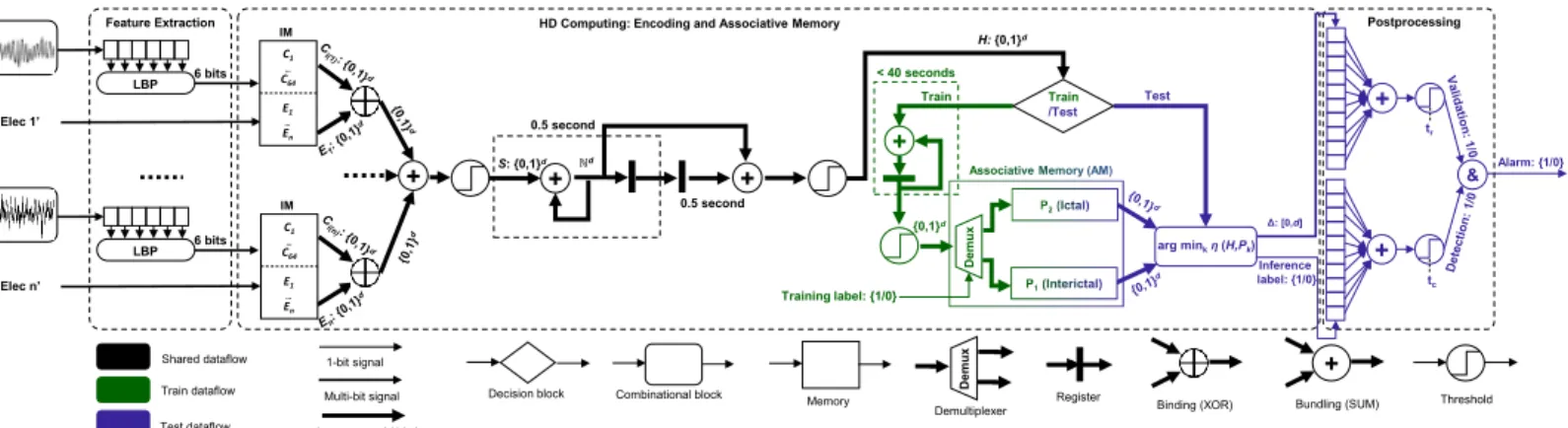
Fig. 1: Processing chain of Laelaps: (1) Feature extraction generates a 6-bit LBP code for each electrode; (2) HD computing maps these codes tod-dimensional atomic vectors and constructs a complex vectorH to represent the histogram of 1 srecording. During training the associative memory (AM) learns from this vector, and during inference provides a label; (3) As postprocessing, a patient-dependent (tr) voting decides based on the last 10 labels and their distance scores (∆).
sample, and generates 26 different symbols that are fed into the next stage for learning and classification (see Fig. 1).
B. Learning and Classification in HD Space
HD computing first applies random embeddings of the LBP codes in the HD space via the IM, which assigns a nearly orthog-onal i.i.d.d-bit vector to every LBP code, i.e., C1⊥C2. . .⊥C64. To combine these vectors across all electrodes, HD computing generates a spatial record (S), in which an electrode name
is treated as a field, and its LBP code as the value of this field. The IM also maps the names of the electrodes to random embeddings nearly orthogonal binary vectors: E1⊥E2. . .⊥En for a patient with n electrodes. This allows to bind (⊕) the name of each electrode (Ej | j ∈ [1, n]) to its corresponding code (Ci(j) | i ∈ [1,64]). This binding (Ej ⊕Ci(j)) gener-ates a new set of nearly orthogonal vectors to represent LBP codes per electrode that effectively reduces the size of IM from
64×n vectors to 64 +n vectors. The spatial record (S) is then constructed by bundling the bound vectors of all electrodes:
S= [E1⊕Ci(1)+E2⊕Ci(2)+...+En⊕Ci(n)]. The bundling operation is well suited for representing sets and multisets.
The d-bit vector S is computed for every new sample, and holographically represents the spatial information about the LBP codes of all the electrodes. The next step is to compute the histogram of LBP codes for a moving window of 1 swith 0.5 s
overlap. To estimate the histogram of LBP codes inside this window, a multiset of temporally generatedSvectors is computed asH = [S1+S2+...+S512]. The bundling operation is applied in the temporal domain through accumulation (i.e., componentwise addition) ofStvectorst∈ {1, ...,512}, that are produced within the window, and then thresholding at half (i.e., normalization). As mentioned in Sec. II-A, the interictal and ictal states are characterized by different distributions of LBP codes that are reflected byH.
The output of the encoding is H, a d-bit vector that is updated every 0.5 s. Note that representation of H, as a com-posite structure, is constructed directly from representations of the atomic vectors by applying the operations in the encoder
without requiring any learning. To train our classifier, we use vector H to build an associative memory (AM) containing two
prototypevectors representing ictal and interictal labels. To train
the interictal prototype, allH vectors computed over an interictal state of 30 s are accumulated (summed), and then thresholded (normalized) to be stored in the AM as ad-bit prototype vector (P1). Similarly, an ictal prototype vector (P2) is generated from an ictal state that can last 10 s to 30 s depending on seizures’ duration. For classification, every 0.5 s, the label of an unseen window is determined by comparing its H to P1 and P2 in the AM. The prototype that results in the minimum Hamming distance (arg minkη(H, Pk)) is the label.
C. Postprocessing
The last part of Laelaps postprocesses the labels and distances produced by the HD classifier for the final decision. For each labeled window, we associate a∆score as the absolute difference between two prototype distances:∆ =|η(H, P1)−η(H, P2)|. We consider a postprocessing window that takes into account the last 10 labels and their corresponding∆ scores (shifting them every 0.5 s). The final decision is made based on two thresholds (tc,tr), the former considers the classification labels and the latter checks their∆scores. Laelaps flags an alarm (as the seizure onset) only if the following two conditions are met: the number of ictal labels inside the postprocessing window ≥tc, and the mean of ∆ of those labels exceedstr.
We set tc = 10 for all the patients, thus flagging a seizure alarm after at least 10 consecutive output labels indicating an ictal state. This increases the detection delay but filters out many false alarms. In contrast,tris tuned for each patient Pi. If there are no
false alarms after filtering based on the hard classification results using tc, we set t
(Pi)
r = min ∆(Pictali) to maximize robustness to
false alarms without affecting the sensitivity. Otherwise, we select
tr as the highest integer multiple ofmax ∆ (Pi)
interictal, such that it remains lower than max ∆(Pi)
ictal−α, where α is the difference between the mean∆ictalacross the samples used to train the HD classifier and the remaining samples in the training set, averaged across all patients. This is used to compensate for the higher confidence of the classifier for the samples on which it was trained.
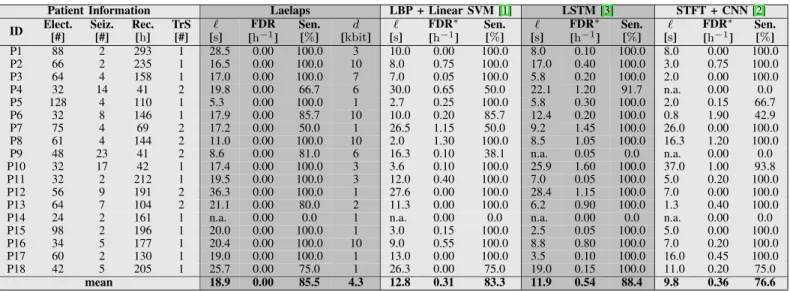
TABLE I: Used abbreviations/symbols: Elect.: number of electrodes, Seiz.: total number of seizures, Rec.: total duration of the recording, TrS: number of seizures used in training,`: delay of seizure onset detection, FDR: false detection rate, Sen.: sensitivity, and n.a. not applicable. Note that FDR∗ is computed only on 20 hthat is randomly selected from interictal test set.
Patient Information Laelaps LBP + Linear SVM[1] LSTM[3] STFT + CNN[2]
ID Elect.[#] Seiz.[#] Rec.[h] TrS[#] [`s] FDR [h−1] Sen. [%] d [kbit] ` [s] FDR∗ [h−1] Sen. [%] ` [s] FDR∗ [h−1] Sen. [%] ` [s] FDR∗ [h−1] Sen. [%] P1 88 2 293 1 28.5 0.00 100.0 3 10.0 0.00 100.0 8.0 0.10 100.0 8.0 0.00 100.0 P2 66 2 235 1 16.5 0.00 100.0 10 8.0 0.75 100.0 17.0 0.40 100.0 3.0 0.75 100.0 P3 64 4 158 1 17.0 0.00 100.0 7 7.0 0.05 100.0 5.8 0.20 100.0 2.0 0.00 100.0 P4 32 14 41 2 19.8 0.00 66.7 6 30.0 0.65 50.0 22.1 1.20 91.7 n.a. 0.00 0.0 P5 128 4 110 1 5.3 0.00 100.0 1 2.7 0.25 100.0 5.8 0.30 100.0 2.0 0.15 66.7 P6 32 8 146 1 17.9 0.00 85.7 10 10.0 0.20 85.7 12.4 0.20 100.0 0.8 1.90 42.9 P7 75 4 69 2 17.2 0.00 50.0 1 26.5 1.15 50.0 9.2 1.45 100.0 26.0 0.00 100.0 P8 61 4 144 2 11.0 0.00 100.0 10 2.0 1.30 100.0 8.5 1.05 100.0 16.3 1.20 100.0 P9 48 23 41 2 8.6 0.00 81.0 6 16.3 0.10 38.1 n.a. 0.05 0.0 n.a. 0.00 0.0 P10 32 17 42 1 17.4 0.00 100.0 3 3.6 0.10 100.0 25.9 1.60 100.0 37.0 1.00 93.8 P11 32 2 212 1 19.5 0.00 100.0 3 12.0 0.40 100.0 7.0 0.05 100.0 5.0 0.20 100.0 P12 56 9 191 2 36.3 0.00 100.0 1 27.6 0.00 100.0 28.4 1.15 100.0 7.0 0.00 100.0 P13 64 7 104 2 21.1 0.00 80.0 2 11.3 0.00 100.0 6.2 0.90 100.0 1.3 0.40 100.0
P14 24 2 161 1 n.a. 0.00 0.0 1 n.a. 0.00 0.0 n.a. 0.00 0.0 n.a. 0.00 0.0
P15 98 2 196 1 20.0 0.00 100.0 1 3.0 0.15 100.0 2.5 0.05 100.0 5.0 0.00 100.0
P16 34 5 177 1 20.4 0.00 100.0 10 9.0 0.55 100.0 8.8 0.80 100.0 7.0 0.20 100.0
P17 60 2 130 1 19.0 0.00 100.0 1 13.0 0.00 100.0 3.5 0.10 100.0 16.0 0.45 100.0
P18 42 5 205 1 25.7 0.00 75.0 1 26.3 0.00 75.0 19.0 0.15 100.0 11.0 0.20 75.0
mean 18.9 0.00 85.5 4.3 12.8 0.31 83.3 11.9 0.54 88.4 9.8 0.36 76.6
IV. DATASET ANDEXPERIMENTALRESULTS
A. Long-term Human iEEG Dataset
Our anonymized dataset comprises 18 patients (P1–P18) from the epilepsy surgery program of the Inselspital Bern. For each patient, the number of seizures varies from 2 to 23, and the total durations of interictal recordings from 41 h to 293 h. Two patients out of 18 (P8 and P14) show a high number of fast and short seizures (70 and 60, respectively), hence we only consider 4 and 2 seizures as the lead seizures [20] for them. The dataset includes a total of2656 hof recording, with 116 seizures marked by an experienced and board-certified epileptologist (K.S.). The first part of Tbl. I shows the number of electrodes, the number of seizures, and the total hours of recordings for every patient.
B. Results: Sensitivity, False Alarms, and Detection Delay
To evaluate the performance of Laelaps, we assess the follow-ing metrics given a few trained seizure examples: (1) sensitivity, defined as number of detected seizures out of the number of test seizures; (2) false detection rate (FDR), defined as the number of false alarms that occurred during an hour; (3) delay of detection, defined as the time distance between the algorithm detection and the expert marked seizure onset. Note that this is measured as the
working delay of algorithms, and not the implementation delay. Implementation results including speed of execution and energy consumption are discussed in Sec. V-C.
We evaluate the performance for a practical clinical setting with the goal of reducing time-to-functioningof an algorithm to get it reliably operational as soon as the first few seizures are observed. Hence, we partition the dataset in chronological order to a training set, covering continuous recording until the end of the first or second seizure depending on the patient (see TrS in Tbl. I), that is followed by a longer testing set until the end of recording. The training set includes 37.7% of total recording on average among the patients. We train patient-specific models by using one or two ictal state(s), ranging from 10 s to 30 s, and one 30 s interictal state that is chosen to be 10 min before the first seizure onset. This training generates the content of AM in Laelaps and weights for other SoA. We also use the rest of
interictal and ictal samples to tunetravailable in the training set at least until the first seizure.
As shown in Tbl. I, Laelaps achieves85.5 % mean sensitivity
(100 % median) among the patients, and an ideal 0.0 h−1 FDR
on 1357 h of test set. In addition, for the majority of patients
(11 out of 18), Laelaps achieves perfect sensitivity (100 %). Note that we have already done cross-validation on a short-time iEEG dataset in [12], and we consistently observed superior sensitivity, specificity, and fast learning benefits; however, cross-validation with this long-term dataset is highly impractical especially for the SoA methods, e.g., the classification time of the LSTM is 2.1×
slower than the real-time on an Intel Xeon CPU at2.4 GHz. We compare Laelaps with the SoA methods in seizure detection including LBP+SVM [1], and LSTM networks [3]. Besides, we consider CNNs coupled with short time Fourier transform (STFT) that is proposed as a universal method for seizure prediction [2]. We apply these methods to our seizure detection task using the same setup but tr= 0. These methods do not attain ideal FDR: SVM comes closest and performs ideally on 4 out of 18 patients (0.0 h−1FDR and100 %sensitivity), but achieves0.31 h−1FDR and83.3 %mean sensitivity among all the patients. The other SoA methods suffer from significantly higher FDR,0.36 h−1with the CNN, and0.54 h−1with the LSTM, which limits their application in long-term recording. Interestingly, Laelaps still maintains a lower FDR of 0.15 h−1 even with tr = 0 (i.e., without any tuning). Note that we were able to compute the FDR for the SoA methods only on 20 hof randomly selected interictal recordings due to their slow inference time. Overall, Laelaps detects 79 out of 92 unseen seizures, while the other methods perform worse: 69, 51, and 69 detected seizures using the SVM, the CNN, and the LSTM, respectively. Noteworthy, only for two patients (P7 and P14), Laelaps shows a very low sensitivity (50% and 0%, respectively). For P7, it could be due to the LBP features as LBP+SVM also reaches the same sensitivity, and for P14, all the SoA methods fail as well.
The average delay of seizure onset detection of Laelaps is slightly larger than the one yielded by the SoA methods (18.89 s
113117 14 popcount 100 1 32 H +1+0+0 +1 32 Co m p u te LB P 128 40 32 11 22 13 63 63 63 39 16 32 0 LBPs 256 IM2 32 32 32 32 IM1 32 32 32 32 1 32 33 64 1000 XOR, transpose 32x32 bit blocks 1 32 33 64 1000 1000 32 ƞ Alarm H AM {1/0}
ENCODING kernel: 32 blocks, 32 threads
LBP kernel: 128 blocks, 256 threads CLASSIFICATION: 1 block, 32 threads
Block 1 T h re a d 1 T h re a d 2 T h re a d m Block 2 Block n Color coding of GPU thread grid
S Add & threshold 0.5 s P1 P2
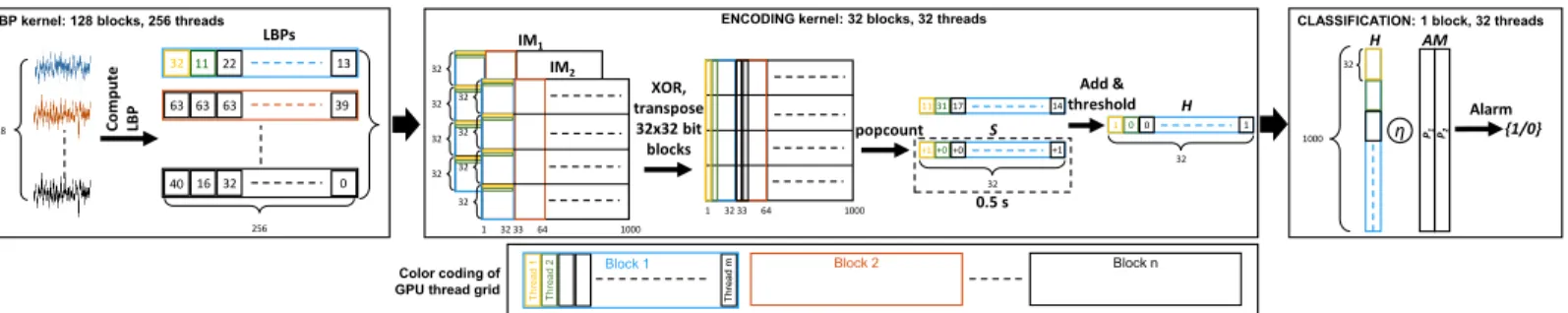
Fig. 2: GPU implementation of Laelaps using three kernels. Different colors indicate different threads and thread blocks.
similar average delay of13.8 son289 hof recording with an FDR of0.13 h−1[11]. Such a detection delay below20 sis still suited for several important applications considering that iEEG seizure onset often precedes clinical onset by more than20 s [21].
Finally, we tune the dimension (d) of the vectors separately for each patient. First, we perform the experiments withd=10 kbit
to build a golden model, and then we reducedas long as the same performance is maintained. As shown in Tbl. I,dis reduced for 14 patients, on average tod= 4.3 kbit, without any performance loss while saving memory, energy, and time.
V. IMPLEMENTATION ON THETEGRAX2 PLATFORM
In this section, we introduce the Nvidia Tegra X2 platform and describe the GPU implementation of Laelaps. We have chosen Tegra X2 to be able to compare the energy consumption and execution time of Laelaps with the SoA methods in the same hardware fabric. However, HD computing naturally fits in ultra-low power nodes (≈2 mW at 28 nm [19]) as well as emerging 3D nanoscalable fabrics [17].
A. Platform Overview
Nvidia’s Tegra X2 platform is an embedded computing SoC targeted at AI workloads. It consists of a dual-core Denver2 ARMv8 CPU, a 4-core ARM Cortex-A57, and a 256-core GPU based on the Pascal architecture, which provides a performance of 750 GFLOPS (single-precision) at a power consumption of around 15 W with a memory bandwidth of 58.4 GB/s. The TX2 has several power modes, among them Max-Q, which allows for the maximum energy efficiency by running the ARM cluster at
1.2 GHz and the GPU at 0.85 GHz. We use this mode for all
our experiments on the Jetson TX2 development board, and the on-board sensors for power measurements.
B. GPU Implementation of Laelaps
We provide an overview of the GPU implementation in Fig. 2 and discuss the individual computing kernels in the following paragraphs. Readers inexperienced in GPU programming can refer to [22].
a) LBP Kernel. The first kernel of Laelaps maps an iEEG window of 256 samples (0.5 s) to its LBP codes. Each LBP value is computed by an independent thread: one thread block per electrode (e.g. 128), and one thread per block for each LBP (i.e. 256). This allows us to exploit data locality within each thread block by copying the corresponding electrode’s data samples to shared memory before computing the LBPs.
b) HD Encoding Kernel. For implementation of the IM we consider two physical IM1and IM2. The computed LBPs are used to index the IM1 for mapping the LBPs to the vectors. Similarly
the electrode index is used to find the corresponding vector in the IM2. The vectors (d= 1 kbit) stored in the IMs are packed into 32 integer variables with 32-bit each (padded, if necessary). With 64 possible LBPs, the IM1 occupies64 kbitand the IM2is
128 kbit. They thus fit entirely into the64 kBof shared memory
available per multiprocessor on the TX2 for fast access, even for the largest model configurations considered herein.
The processing is done by 32 thread blocks, one for each 32-bit chunk of the vector independently, with 32 threads each. After loading the IMs to the shared memory, the threads within each block: 1) load the vector related to the LBP code, 2) load the vector for the corresponding electrode, and 3) perform the XOR operation on them. Each of these steps takes one cycle on the TX2’s GPU. The threads are then synchronized.
At this point and for each thread block, we have 32 threads, each storing a single 32-bit word. This 32 × 32-bit matrix is now transposed (using bit-masking and __ballot_sync
instructions). A single popcount instruction is then used to sum the contribution of 32 electrodes in each thread. This is repeated until all electrodes’ contributions are accumulated (e.g., 4 times for 128 electrodes).
Once this execution is completed, the results are binarized producing S that is further accumulated over 256 time steps (0.5 s), and stored as a partial sum. This result is added to the one of the previous iteration (i.e. creating the window of1 s) and then again binarized, forming thed-bit vectorH that can be used for learning and classification.
c) Classification Kernel. In the last kernel, the vector H is compared to the two prototype vectors in the AM, determining the Hamming distance to each of them, and the aforementioned (Sec. III-C) postprocessing is applied by the master thread. This is a computationally negligible step and is only parallelized across a single thread block of 32 threads.
C. TX2 Measurements: Inference Speed and Energy
To measure the speed and energy of different methods dis-cussed in Section IV, we consider an identical scenario: each model is trained offline and is loaded into the TX2 memory together with a 30 min interictal state followed by one seizure event. The model is then run on this data sequence, and the execution time and energy consumption for a single classification event are measured.
The SoA methods are implemented using optimized libraries and frameworks, specifically Keras for deep learning approaches (relying itself on Nvidia’s highly optimized cuDNN library) and Scikit-learn for the SVM. We use various combinations of resources (GPU and/or CPU) to find the best performance for
Laelaps (LBP+HD) LBP+SVM LBP+SVM STFT+CNN STFT+CNN LSTM LSTM False Detect ion Rate [#/h ou r]
Energy per classification [mJ]
Better
Fig. 3: Comparing the methods in terms of false detection rates and energy consumption with 64 electrodes on the TX2 in the Max-Q power mode. Legend:CPU,GPU.
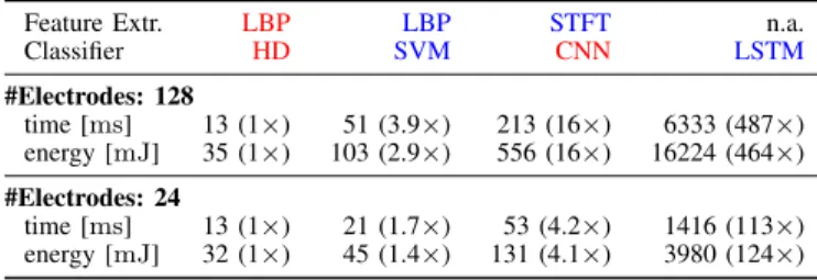
TABLE II: Energy and inference time of Laelaps, SVM, CNN, and LSTM for one classification event. Legend:CPU,GPU.
Feature Extr. LBP LBP STFT n.a.
Classifier HD SVM CNN LSTM #Electrodes: 128 time [ms] 13 (1×) 51 (3.9×) 213 (16×) 6333 (487×) energy [mJ] 35 (1×) 103 (2.9×) 556 (16×) 16224 (464×) #Electrodes: 24 time [ms] 13 (1×) 21 (1.7×) 53 (4.2×) 1416 (113×) energy [mJ] 32 (1×) 45 (1.4×) 131 (4.1×) 3980 (124×)
each of the SoA methods. Fig. 3 compares the mean FDR of all the patients, and energy consumption per every0.5 sclassification event using 64 electrodes as the median number electrodes among the patients. It highlights that the SVM requires up to 2 orders of magnitude less energy with lower FDR compared to the deep learning methods, confirming its usage in the wearable EEG-based seizure detection devices [7]. Laelaps remarkably surpasses the SVM by 1.9×lower energy and zero false alarms.
In Tbl. II, we further analyze these aspects for two electrode configurations: 24 electrodes as the minimum number of elec-trodes among patients (P14), and 128 as the maximum (P5). We show the results of a single implementation of each method, either on the CPU, GPU, or a combination of them, that results in minimal energy consumption (note that LSTM is memory bound while CNN is compute bound).
With the 24-electrode model, Laelaps takes12.5 msand32 mJ
achieving 1.7×faster classification and 1.4×lower energy con-sumption compared to the SVM. Laelaps achieves a speed-up of 4.2×–113×and an energy saving of 4.1×–124×with respect to deep learning algorithms.
We also evaluate the scalability by increasing the number of electrodes to 128. Laelaps’s savings (in both time and energy) are magnified: 3.9×(2.9×) faster execution (lower energy) with respect to the SVM, and 16×–487× (16×–464×) compared to the deep learning methods. These results indicate almost constant execution time and energy consumption of Laelaps with respect to the number of electrodes (12.5 mswith 24 electrodes vs.13.0 ms
with 128 electrodes, and 32.0 mJ vs. 35.0 mJ). In contrast, the SoA methods exhibit a linear growth at least in both these metrics
(e.g., 20.8 ms vs. 51.0 ms, and 44.8 mJ vs. 103.0 mJ in SVM), thus implying better scalability of Laelaps for more electrodes.
VI. CONCLUSION
Laelaps—on our very large dataset with 116 seizures in2656 h
of continuous recording from 18 epilepsy patients implanted with 24 to 128 intracranial EEG electrodes—simultaneously reduces the following metrics compared to LBP+SVM, STFT+CNN, and LSTM: the number of undetected seizures, false alarms (to zero), execution time and energy consumption for classification on a TX2 embedded device. Our future work will focus on designing specialized hardware for Laelaps and on reducing the delay.
ACKNOWLEDGMENT
Support was received from the ETHZ Postdoctoral Fellowship Program, the Marie Curie Actions for People COFUND Program, and the EU’s H2020 under grant No. 780215.
REFERENCES
[1] A. K. Jaiswalet al., “Local pattern transformation based feature extraction techniques for classification of epileptic EEG signals,” Biomedical Signal Processing and Control, pp. 81–92, 2017.
[2] N. D. Truonget al., “Convolutional neural networks for seizure prediction using intracranial and scalp electroencephalogram,”Neural Networks, pp. 104–111, 2018.
[3] R. Husseinet al., “Robust detection of epileptic seizures using deep neural networks,” inProc. IEEE ICASSP, 2018.
[4] S. N. Baldassanoet al., “Crowdsourcing seizure detection: algorithm devel-opment and validation on human implanted device recordings,”Brain, pp. 1680–1691, 2017.
[5] P. P. M. Shaniret al., “Automatic seizure detection based on morphological features using one-dimensional local binary pattern on long-term EEG,” Clinical EEG and Neuroscience, pp. 351–362, 2018.
[6] D. Sopic et al., “e-Glass: A wearable system for real-time detection of epileptic seizures,” inIEEE ISCAS, May 2018, pp. 1–5.
[7] M. A. B. Altafet al., “A 1.83µj/classification, 8-channel, patient-specific epileptic seizure classification SoC using a non-linear support vector ma-chine,”IEEE TBioCAS, pp. 49–60, Feb 2016.
[8] J. van Andelet al., “Multimodal, automated detection of nocturnal motor seizures at home: Is a reliable seizure detector feasible?”Epilepsia Open, pp. 424–431, Dec 2017.
[9] D. M. Goldenholzet al., “Long-term monitoring of cardiorespiratory pat-terns in drug-resistant epilepsy,”Epilepsia, pp. 77–84, 2017.
[10] O.-Y. Kwonet al., “Depression and anxiety in people with epilepsy,”Journal of Clinical Neurology, pp. 175–188, 2014.
[11] W. Zhouet al., “Epileptic seizure detection using lacunarity and bayesian linear discriminant analysis in intracranial EEG,”IEEE TBME, Dec 2013. [12] A. Burrello et al., “One-shot learning for iEEG seizure detection using
end-to-end binary operations: local binary patterns with hyperdimensional computing,” inIEEE BioCAS, 2018.
[13] C. S. Daw et al., “A review of symbolic analysis of experimental data,” Review of Scientific Instruments, pp. 915–930, 2003.
[14] K. Schindleret al., “On seeing the trees and the forest: Single signal and multi signal analysis of periictal intracranial EEG,”Epilepsia, 2012. [15] K. Schindler et al., “Ictal time-irreversible intracranial EEG signals as
markers of the epileptogenic zone,” Clinical Neurophysiology, pp. 3051– 3058, 2016.
[16] P. Kanerva, “Hyperdimensional computing: An introduction to computing in distributed representation with high-dimensional random vectors,”Cognitive Computation, pp. 139–159, 2009.
[17] A. Rahimiet al., “High-dimensional computing as a nanoscalable paradigm,” IEEE Transactions on Circuits and Systems I, Sept 2017.
[18] A. Rahimi et al., “Hyperdimensional computing for noninvasive brain– computer interfaces: Blind and one-shot classification of EEG error-related potentials,”Proc. ACM/EAI BICT, 2017.
[19] F. Montagnaet al., “PULP-HD: accelerating brain-inspired high-dimensional
computing on a parallel ultra-low power platform,” in Proc. ACM/IEEE
DAC, 2018.
[20] B. H. Brinkmannet al., “Crowdsourcing reproducible seizure forecasting in human and canine epilepsy,”Brain, pp. 1713–1722, 2016.
[21] H. Martinet al., “Latencies from intracranial seizure onset to ictal tachy-cardia: A comparison to surface EEG patterns and other clinical signs,” Epilepsia, pp. 1639–1647, 2015.
[22] A. Lefohnet al., “Beyond programmable shading (parts I and II),” inACM SIGGRAPH 2009 Courses, 2009, pp. 1–312.