Block Structure Multivariate Stochastic Volatility Models

Block Structure Multivariate Stochastic Volatility Models

Manabu Asai* Faculty of Economics Soka University Japan Massimiliano Caporin†

Department of Economics and Management “Marco Fanno” University of Padova

Italy

Michael McAleer‡ Econometric Institute Erasmus University Rotterdam Erasmus School of Economics

and Tinbergen Institute

The Netherlands

EI 2009-51

First draft: June 2007 Revised: December 2009

* _{Corresponding author: 1-236 Tangi-cho, Hachioji, Tokyo 192-8577, Japan, tel. +81-42-691-8163, email:} [email protected]

† _{Dipartimento di Scienze Economiche “Marco Fanno” – Università degli Studi di Padova – Via del} Santo, 33 – 35123 Padova, tel. +39-049-8274258, email: [email protected]

‡ _{The third author is most grateful for the financial support of the Australian Research Council, National} Science Council, Taiwan, and Center for International Research on the Japanese Economy (CIRJE), Faculty of Economics, University of Tokyo. [email protected]

Abstract

Most multivariate variance models suffer from a common problem, the “curse of

dimensionality”. For this reason, most are fitted under strong parametric restrictions that

reduce the interpretation and flexibility of the models. Recently, the literature has focused

on multivariate models with milder restrictions, whose purpose was to combine the need

for interpretability and efficiency faced by model users with the computational problems

that may emerge when the number of assets is quite large. We contribute to this strand of

the literature proposing a block-type parameterization for multivariate stochastic

volatility models.

Keywords: block structures; multivariate stochastic volatility; curse of dimensionality

1. Introduction

Classical portfolio allocation and management strategies are based on the assumption that

risky returns series are characterized by time invariant moments. However, the

econometric literature of the last few decades demonstrated the existence of dynamic

behaviour in the variances of financial returns series. The introduction of such empirical

evidence may constitute an additional source of performance for portfolio managers, as

evidenced by Fleming, Kirby and Ostdiek (2001), or may be relevant for improving the

market risk measurement and monitoring activities (see, for example, Hull and White

(1998) and Lehar et al. (2002)). Two families of models emerged in the literature, namely

GARCH-type specifications (see Engle (2002)), and Stochastic Volatility models (see

Taylor (1986) and Andersen (1994)).

However, portfolio management strategies often involve a large number of assets

requiring the use of multivariate specifications. Among the possible alternative models,

we cite the contributions of Bollerslev (1990), Engle and Kroner (1995), Ling and

McAleer (2003), Asai and McAleer (2006, 2009), and the surveys in McAleer (2005),

Bauwens, Laurent and Rombouts (2006), and Asai, McAleer and Yu (2006). Most models,

if not all, suffer from a common problem, the well-known “curse of dimensionality”,

whereby models become empirically infeasible if fitted to a number of series of moderate

size (in some cases, the models may become computationally intractable with even 5 or 6

assets). In order to match the need of introducing time-varying variances with practical

VECH specifications suggested by Bollerslev et al. (1988), the scalar VECH and BEKK

models proposed by Ding and Engle (2001), the CCC model of Bollerslev (1990), and the

dynamic conditional correlation models of Engle (2002) and Tse and Tsui (2002).

However, the introduction of significant and strong restrictions reduces the interpretation

and flexibility of the models, possibly affecting the purportedly improved performance

they may provide and/or the appropriateness of the analysis based on their results.

Recently, the literature has focused on multivariate models with milder restrictions, whose

purpose was to combine the need for interpretability and efficiency faced by model users

with the computational problems that may emerge when the number of assets is quite

large. Among the contributions in this direction, we follow the approach of Billio,

Caporin and Gobbo (2005). They proposed specifying the parameter matrices of a general

multivariate correlation model in a block form, where the blocks are associated with

assets sharing some common feature, such as the economic sector. Our purpose is to adopt

this block-type parameterization and adapt it to multivariate stochastic volatility models.

In general terms, Multivariate Stochastic Volatility (MSV) models have a parameter

number of order O(n2), where n is the number of assets. With the introduction of block

parameter matrices, we may control the number of parameters and obtain a model

specification which is feasible, even for a very large number of assets. Furthermore, as in

the contribution of Billio et al. (2005), the models we propose follow the spirit of

sectoral-based asset allocation strategies since they will presume the existence of

common dynamic behaviour within assets or financial instruments belonging to the same

factor driving all the variances and covariances, since the financial theory may suggest the

existence of sector-specific risk factors (sectoral asset allocation is often followed by

portfolio managers and characterized by a number of managed financial instruments).

As distinct from an extremely restricted model, we also recover part of the spillover effect

between variances, which allows monitoring of the interdependence between groups of

assets, an additional element which may be relevant. Within our modeling approach, the

coefficients may be interpreted as sectoral specific, while the assets will be in any case

characterized by a specific long term variance through the introduction of unrestricted

constants in the variance equations.

Clearly, the restrictions proposed may not necessarily be accepted by the data, as more

‘complete’ models will, in general, provide better results. We will show that the

introduction of such restrictions provides limited losses, while yielding a significant

improvement over the more restricted specifications. We will evaluate and compare the

alternative models following the Monte Carlo likelihood (MCL) estimation approach for

both univariate and multivariate SV models, as in Sandmann and Koopman (1998) and

Asai and McAleer (2006).

The plan of the remainder of the paper is as follows. Section 2 presents the block-structure

modelling approach within a general MSV framework, and also compares the model to

Factor SV specifications, and addresses some estimation issues. Section 3 presents an

empirical example based on US stock market data for selected firms. Section 4 gives some

2. MSV Models

The block-structure model we present can be considered as a restricted specification of a

general MSV model. In fact we will show how the modelling approach consists in

defining a set of parametric restrictions that makes the model feasible, but without losing

the interpretation of coefficients.

Consider a general MSV model that will be used as reference model. Let R_t be the return series on an asset, and define y_t R_tE R



_t _t1



as the mean-adjusted return. Then, the basic SV model is defined as





 



2



1 exp 0.5 , 0,1 , , 0, , t t t t t t t t y h N h h N _           (1)

where E



 

_{t s}



0 for all t and s. By setting g_t  h_t , where 2 ln , we have an alternative representation, namely y_t 



_texp 0.5



g_t



and g_t1 

 



g_t

 



 _t.

For the M-dimensional stochastic vector, the MSV model of Harvey, Ruiz and Shephard (1994) is defined by





 













1,





2,





,





, 0, , diag ,

diag exp 0.5 exp 0.5 , exp 0.5 ,...exp 0.5 ,

t t t t t t t t M t y DD N P D D h diag h h h        (2)

where P is the correlation matrix,



is the M-vector of standard deviation parameters, and h_t is M-vector of the stochastic components, which follows a VAR(1) process given as





1 , 0, , t t t t h h N          (3)

where the operator _ denotes the Hadamard (or element-by-element) product,  is an

M-dimensional coefficient vector and _ is the covariance matrix. For convenience, we call this type of MSV model the ‘basic MSV’ model.

In the following, we present a closely related specification, the Factor MSV model, and

then we introduce the Block-Structure MSV model.

2.1. Factor MSV model

extended by Jacquier et al. (1995, 1999), and Chib et al. (2006), among others. The basic

model has the following structure:













 





2 2 2 1 2 , , , , , 1 , , 2 , 0, diag , ,... , exp 0.5 , 1, 2,... 0,1 , , 0, , t t t t M i t i t i t i t i t i i t i t t k y Df N f h i k N h h N I _                   (4)

where D is the m k matrix of factor loadings, f_t is the k-dimensional vector of factors, which follow univariate SV models, and all the innovation terms are mutually

uncorrelated. This model has a limited number of parameters, but also has some

drawbacks. In fact, as shown in Asai et al. (2008), the conditions imposed on the mean

innovations,_t, that is, homoscedasticity and diagonality of the covariance matrix, are too restrictive and not consistent with the empirical evidence. This is particularly evident

when the number of factors, k, is much smaller than the number of assets, M. In this case, if the assets are used to create a portfolio, there must exist at least one vector of weights

2.2. Block Structure Model

We now assume that the M assets are divided into B groups, with the i-th group containing

i

m assets (M m₁m₂ _ m_B). We define a block structure for the volatility by assuming that each group of assets is characterized by a common parametric behaviour in

the volatility equation. Consider the variance dynamics of the Harvey et al. (1994) model

in equations (1)-(3):





1 , 0, , t t t t h h N _        (5)

where the matrix of parameters of persistence, , and the covariance matrix of log-volatility, _, will have constraints given by block structures. We define

1 2 1 1 2 1 2 1 2 2 1 2 1 2 ,11 ,21 , , 1 , ,21 , ,22 , 2 , , 1 , , 2 , , , , B B B B B B m m B m u m u m m u B m m u m m u m u B m m u B m m u B m m u BB m I O O O O I O O O O O O O O I I L L L I L L L I                                                      (6)

the number of assets in each block is the same, namely m_iM B , we have



1



diag , ,_B I_M

    and    _{ u} I_M , where  _u

 

_{u ij,} , and  is the Kronecker product. By construction, the vector of volatilities has a block-structure given that the factors affecting the overall volatilities are sector or block specific. Hereafter, we refer to

the model in equations (2), (5) and (6) as the Volatility Block Structure (VBS) MSV

model.

For convenience, we will show the structure of each block in detail. Denote the vector of

filtered returns of the i-th group as



₁ ,  ₂ , ,  



i

i i i

it t t m t

y  y y _ y , where y _jti is the filtered return of the j-th asset in the i-th group. Similarly, denote



₁ , ₂ , ,  



i

i i i

it t t m t

h  h h _ h . For the mean-adjusted returns of the i-group, we have the following structure:





 













, 1 , , 0, , diag , diag exp 0.5 , 0, , i it i it t t i i i it it i t i it it it u ii m y D D N P D D h h h u u N I            (7)

where P_i is the correlation matrix,



₁ , ,  



i

i i

i m

   _ , and  _ji , _i and _{u ii,} are scalar parameters. We refer to this as the ‘one-block SV’ model.

Now we turn to the vector of volatilities of the i-th block, which is defined as









diag exp 0.5

it i it

Thus, the vector of volatilities for all assets is given by v_t



v₁_t,_,v_Bt



. We specify the mean equation of y_t 



y₁_t,_,y_Bt



 as





, 0, t t t t y V  N P , (9)

where V_t diag

 

v_t , and P is the correlation matrix.

The numbers of parameters in  



₁,_,_B



 and P are M and M M



1 2



, respectively. For the equation of the main components, the numbers of parameters in  and _u are B and B B



1 2



, respectively. When M 12 and B4 (M 50 and

5

B ), the number of parameters in the BS-MSV model is 92 (1295). For the MSV model of Harvey, Ruiz and Shephard (1994), the number of parameters for the case M 12

(M 50) is 168 (2600). Thus, the BS-MSV model is parsimonious in terms of the number of parameters.

The BS-MSV model still suffers from the number of parameters, which increases with the

speed of M2. Thus, we propose the Complete BS (CBS) model, which consists of equations (2), (5) and (6), subject to the restriction:

1 12 12 1 1 12 12 2 2 2 1 1 2 2 B B B B B B B B B P q J q J q J P q J P q J q J P       _{ }            (10)

where P_i

 

p _jki and Q

 

q_lm are the m m_i _i and B B correlation matrices, respectively, and J_ij is an m m_i _j matrix of ones. In this model, Q captures the correlations between the blocks. As the number of parameters in P is given by









1 1 2 1 2 B i i i B B m m 

 



 , the CBS-MSV model has 2





1 1 2 B i i i M B B m m    





parameters. In the limiting case of blocks characterized by the same number of assets,

when 12M  and B4 (M 50 and B5), the number of parameters in the CBS-MSV model is 56 (305). Therefore, the CBS model drastically reduces the number

of parameters. With the further restriction that p _jki  p i , the CBS-MSV model has

2

2

M  B B parameters. In this case, assuming again that each block includes M/B series, 12M  and B4 (M 50 and B5) yields 36 (85) parameters.

Note that similar block structures could be used for the specification of the factor loading

matrix, D, of the model in (4). In this alternative representation, the latent factors could be associated with the specific blocks created with the assets. Alternatively, making the D matrix unrestricted, block specifications could be used to generalize the model in (4) by

introducing spillovers across the factor variances and by removing the diagonality

2.3 Model estimation

For the estimation of the MSV models, we use the Monte Carlo likelihood (MCL)

approach proposed by Durbin and Koopman (1997). Sandmann and Koopman (1998)

applied the MCL method to the univariate SV model, while Asai and McAleer (2006)

adapted it for the MSV model. These two papers rely on the logarithmic transformation of

squared returns, as in Harvey, Ruiz and Shephard (1994), allowing a state-space form with

non-Gaussian measurement errors. In the MCL method, the likelihood function can be

approximated arbitrarily by decomposing it into a Gaussian part, which is constructed by

the Kalman filter, and a remainder function, for which the expectation is evaluated

through simulation.

3. Empirical analysis

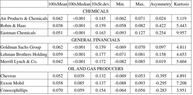
Three groups of three assets from three different sectors (B=3 and M=9) are used, namely Chemical, General Financials, and Oil and Gas Producers. Table 1 reports the selected

stocks and a descriptive analysis of their returns. These assets have been selected from

among a small list of the largest companies between each sector on the basis of the

correlations between the squared returns. All the selected stocks belong to the large cap

segment of the NYSE, and enter the S&P 500 index. Given the approach followed in the

asset selection, intuitively there possibly exist common patterns in the variances. We

chose such a selection approach in order to provide an example where the proposed

modelling approach may be useful. We believe that the block structur MSV model may be

characterized by low correlations.

The series considered are total return indices, collected in the sample period 2 January

2002 to 10 April 2007, giving T=1375 observations. Note that the period covered excludes the effects of the technology market drawdown, while it may be influenced by

the wars in Afghanistan and Iraq and by the increasing trend in oil prices. Furthermore, we

exclude the global financial crisis period.

Table 1 reports a preliminary descriptive analysis of the 9 stocks, showing that in the

period considered the average returns are positive (the stock market was characterized by

an upward trend in prices), and very close between assets of the same sector, while there is

a slight difference between sectors: the chemical sector has lower returns than the general

financial sector which is, in turn, dominated by the oil and gas producer sector. This is a

somewhat expected result, given the relevant increase in the oil prices in the later years of

the sample. The standard deviations of the oil sectors are the smallest, while the General

Financial sector has the highest risk. The Chemical sector has the most leptokurtic

densities; the Oil and Gas Produces stocks are negatively skewed, while the others are all

positively skewed, a fact that is also reflected in the median returns.

The correlations within each sector are quite high, around 0.65 for the Chemical sector,

about 0.8 for the General Financial stocks, and close to 0.75 for the Oil and Gas Producers

firms. Between sectors, the correlations are lower and vary between 0.32 and 0.54.

Notably, the correlations between assets of different sectors have a block-like structure:

higher than the correlations between a chemical and an oil producer firm, at around 0.4.

Finally, the correlations between a general financial firm and an oil producer firm are

again close to 0.4.

In order to develop the conditional mean for each return, we used the following data sets;

a set of interest rates (US Treasury bond 3 months, 6 months, 9 months, 1-3 years, 3-5

years, 5-7 years), oil prices, and two dummies (January and Monday). Interest rates are in

the form of bond indices. Following Ait-Sahalia and Brandt (2001) and Pesaran and

Timmerman (1995, 2000), we fit the conditional mean returns with the constant term, the

lagged return, the contemporaneous dummies, the lagged Oil returns, and the deviations

between the returns of the rates (the following differences between bond indices returns: 6

months minus 3 months, 1-3 years minus 6 months, and so on), giving 10 explanatory

variables, as follows:

 

1 2 1 3 4 5 6 1 10 5

Jan Mon Oil

t t t t t t t

E R 

 

 R_ 



D 



D 



R 



V  _



V .

The deviations between the rates, V_it, can be considered as a proxy for the curvature of the yield curve, and hence may be useful in predicting stock movements.

In the proposed equation, the curvature of the yield curve and the oil returns are

contemporaneous. Clearly, the model may suffer from simultaneity problems, given that

the explanatory variables may be predictable, and we are not including an appropriate

equation for their behaviour. In order to validate the returns model, we run a set of

bidirectional causality. In the first case, we run standard causality tests based on a lagged

relation between variables for all pairs of stock returns and explanatory variables. In all

cases we have limited evidence of causality (few tests have p-values below 0.2, and none

is below 0.05).

In order to implement the bidirectional causality test, we estimated two simultaneous

systems, the restricted version without contemporaneous feedback from the explanatory

variables to the stocks. In this case (we have 54 restrictions, 6 restrictions on each

equation, the 5 variables related to the bonds and the oil price, for the 9 stocks), the

restricted likelihood is 97571.22, the full likelihood is 97605.34, and the LR test statistic

is 68.24. Assuming an asymptotic density following a chi-square distribution with 54

degrees of freedom, we have a p-value of 0.092. We interpret this result as a rejection of

the bidirectional causality (even if the decision was not extremely clear). Given the

outcome of the tests, we can safely run the analysis on the equation with a

contemporaneous relationship.

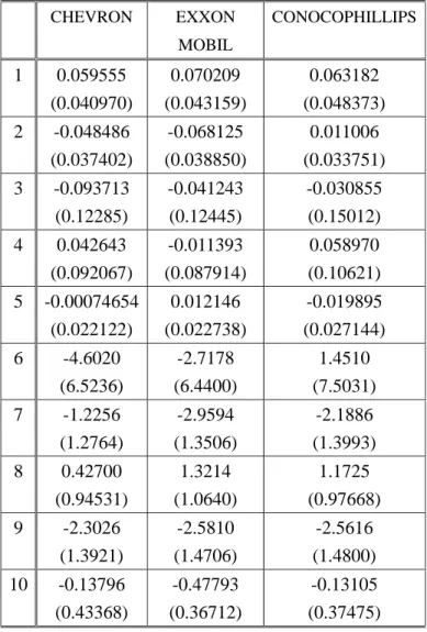
Table 2 gives the results for the conditional mean equation. The number in the first column

denotes the corresponding explanatory variable. For instance, #1 is the constant term, and

# 2 is the AR(1) coefficient. The heteroskedasticity consistent standard errors are given in

parentheses. Although most of the parameter estimates are insignificant, there are some

exceptions, such as R_t and V_2t for AIR PRDS. & CHEMS.

For the volatility equation, we first estimated the univariate SV models defined in

estimates of  for the financial sector are relatively low, the estimates are typical of those available in the literature for SV models. Furthermore, we note a similarity between the

volatility constants, σ, associated with the stocks belonging to the same sector.

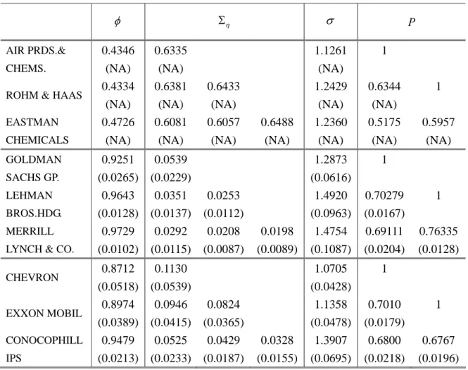
We also estimated the basic trivariate SV models (2) and

Error! Reference source not found. for the three sectors, and Table 4 presents the results.

By introducing the off-diagonal elements of _ and P, the estimates of  are smaller than the corresponding estimates in Table 3 for all the sectors. The correlation coefficients

based on _ are very high and replicate the ordering of Table 1, with the Chemical sector characterized by lower correlations between assets. As the estimate for  is very close

to a singular matrix for the chemical sector, the standard errors are unreliable, and hence

are not reported. As the values of  are close to each other in each sector, and since the estimates of _ indicate the existence of common movements in _t, we need to consider common structures by using factor models and/or the BS models.

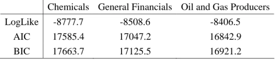
Table 5 shows the log-likelihood, AIC and BIC for the trivariate SV model. Comparing

these values with those in Table 3, we conduct an LR test for the off-diagonal elements of



 and P. The test statistic has a



2

 

6 asymptotic density, and we are able to reject the null hypothesis that all the off-diagonal elements of _ and P are equal to zero for all three sectors.

the three sectors. Table 6 shows the MCL results for the one-block model. Due to the BS

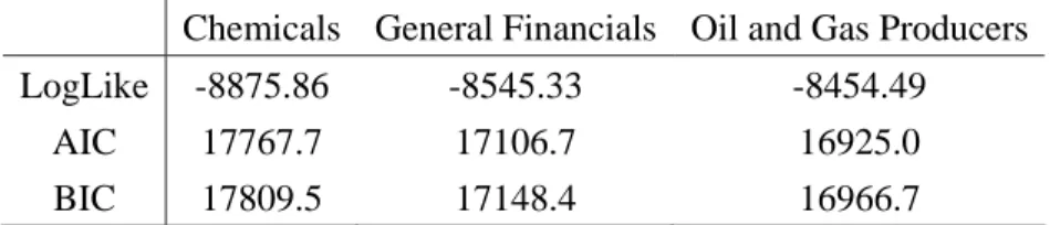
approach, the estimates of  are less than the smallest values of the corresponding sector in Table 3. Table 7 gives the log-likelihood, AIC and BIC for the one-block model. The

one-block model for the chemical sector has smaller AIC and BIC values than the basic

MSV model in (2) and Error! Reference source not found.. For the remaining two

sectors, BIC favours the one-block model, while AIC chooses the basic MSV model. As a

result, we find that the BS approach would be a good candidate for effectively reducing

the number of parameters for high dimensional models.

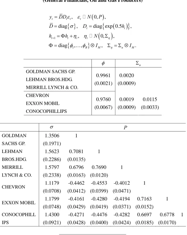
Next, we consider the 6-variate SV model with 2 blocks. Tables 8-10 show the MCL

estimates for the combination of sectors {(General Financials, Oil and Gas Producers),

(General Financials, Chemicals) and (Oil and Gas Producers, Chemicals)}. With respect

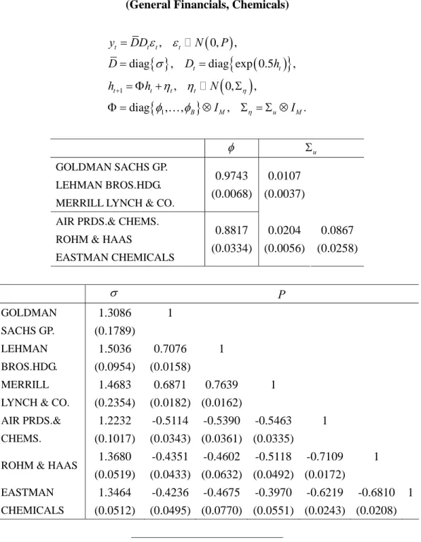
to Tables 9 and 10, the estimates of  became relatively low by including the chemical sector. Finally, we report in Table 11 the estimates of the full 9-variate model with three

blocks associated with the three economic sectors. The parameter estimates are in line

with those reported in Tables 8-10.

A direct comparison of the BS specifications with the full model estimate is not directly

available due to the computation complexity of the 6-variate and 9-variate full models.

Only three-variate specifications are available, both in their full and BS specifications,

and standard likelihood ratio tests clearly favour the full models. However, when the

cross-sectional dimensions increase, the BS specifications remain feasible, while the full

SV models are not. This is a particularly strong advantage of the model presented in the

innovations as the matrices P and _ are not restricted to be diagonal or block-diagonal.

A more detailed comparison of the full and BS specifications for stochastic volatility

models is left to future research.

4. Conclusion

In this paper we presented a class of multivariate stochastic volatility models which is

nested in the model of Harvey et al. (1994). A distinctive feature of our model is that,

contrary to fully parameterized MSV models, it remains feasible in moderate to large

cross-sectional dimensions. This result is achieved by imposing a block structure on the

model parameter matrices. The variables could be grouped by using some economic or

financial criteria, or could follow data-driven classifications. In addition, by the

introduction of blocks, if these have an economic interpretation, the model proposed

preserves the interpretation of the coefficients, a feature which is generally lost in feasible

MSV models.

We also presented an empirical application where the proposed model was estimated for a

set of US equities, showing its feasibility. A more advanced comparison between the BS

References

Ait-Sahalia, Y., and M.W. Brandt (2001), Variable selection for portfolio choice, Journal

of Finance, 54-4, 1297-1351

Asai, M. and M. McAleer (2006), Asymmetric multivariate stochastic volatility,

Econometric Reviews, 25, 453-473.

Asai, M. and M. McAleer (2009), The structure of dynamic correlations in multivariate

stochastic volatility models, Journal of Econometrics, 150, 182--192.

Asai, M., M. McAleer and J. Yu (2006), Multivariate stochastic volatility: A review,

Econometric Reviews, 25, 145-175.

Andersen, T.G. (1994), Stochastic autoregressive volatility: A framework for volatility

modeling, Mathematical Finance, 4, 75-102.

Bauwens, L., S. Laurent and J.V.K. Rombouts (2006), Multivariate GARCH: A survey,

Journal of Applied Econometrics, 21, 79-109.

Billio, M., M. Caporin and M. Gobbo, (2006), Flexible dynamic conditional correlation

multivariate GARCH for asset allocation, Applied Financial Economics Letters, 2,

Bollerslev, T., R.F. Engle and J.M. Wooldridge, (1988), A capital asset pricing model with

time varying covariances, Journal of Political Economy, 96, 116-131

Bollerslev T., (1990), Modelling the coherence in short-run nominal exchange rates: A

multivariate generalized ARCH approach, Review of Economic and Statistics, 72,

498-505.

Chib, S., F. Nardari and N. Shephard (2006), Analysis of high dimensional multivariate

stochastic volatility models, Journal of Econometrics, 134, 341-371.

Ding, Z. and R.F. Engle, (2001), Large scale conditional covariance matrix modeling,

estimation and testing, Academia Economic Papers, 29-2, 157-184.

Durbin, J. and S.J. Koopman (1997), Monte Carlo maximum likelihood estimation for

non-Gaussian state space models, Biometrika, 84, 669-684.

Engle, R.F. (2002), Dynamic conditional correlations - a simple class of multivariate

GARCH models, Journal of Business and Economic Statistics, 20, 339-350.

Engle R.F. and K.F. Kroner (1995), Multivariate simultaneous generalized ARCH,

Econometric Theory, 11, 122-150.

Fleming, J., C. Kirby and B. Ostdiek (2001), The economic value of volatility timing,

Harvey, A.C., E. Ruiz and N. Shephard (1994), Multivariate stochastic variance models,

Review of Economic Studies, 61, 247-264.

Hull, J. and A. White (1998), Incorporating volatility up-dating into the historical

simulation method for VaR, Journal of Risk, 1, 5-19.

Jacquier, E., N.G. Polson and P.E. Rossi (1995), Models and priors for multivariate

stochastic volatility, CIRANO Working Paper No. 95s-18, Montreal.

Jacquier, E., N.G. Polson and P.E. Rossi (1999). Stochastic volatility: univariate and

multivariate extensions, CIRANO Working paper 99s-26, Montreal.

Lehar, A., M. Scheicher and C. Schittenkopf (2002), GARCH vs. stochastic volatility:

Option pricing and risk management, Journal of Banking and Finance, 23, 323-345.

Ling, S. and M. McAleer (2003), Asymptotic theory for a vector ARMA-GARCH model,

Econometric Theory, 19, 278-308.

McAleer, M. (2005), Automated inference and learning in modeling financial volatility,

Econometric Theory, 21, 232-261.

Pesaran, M.H. and A. Timmerman (1995), Predictability of stock returns: Robustness and

Pesaran, M.H. and A. Timmerman (2000), A recursive modeling approach to predict UK

stock returns, Economic Journal, 110-460, 159-191.

Sandmann, G. and S.J. Koopman (1998), Estimation of stochastic volatility models via

Monte Carlo maximum likelihood, Journal of Econometrics, 87, 271-301.

Taylor, S.J. (1986), Modelling Financial Time Series, Chichester, Wiley.

Tse, Y.K. and A.K.C. Tsui, (2002), A multivariate GARCH model with time-varying

Table 1: Descriptive Statistics, and Covariance and Correlation Matrices

Panel a: Descriptive Statistics

100xMean 100xMedian 10xSt.dev. Min. Max. Asymmetry Kurtosis CHEMICALS

Air Products & Chemicals 0.042 <0.001 0.145 -0.062 0.071 0.024 5.119 Rohm & Haas 0.038 <0.001 0.159 -0.058 0.082 0.422 5.443 Eastman Chemicals 0.051 <0.001 0.163 -0.093 0.127 0.254 9.957

GENERAL FINANCIALS

Goldman Sachs Group 0.062 <0.001 0.159 -0.069 0.070 0.097 4.811 Lehman Brothers Holding 0.059 <0.001 0.177 -0.071 0.081 0.158 4.653 Merrill Lynch & Co. 0.042 <0.001 0.172 -0.082 0.085 0.019 5.604

OIL AND GAS PRODUCERS

Chevron 0.052 0.039 0.132 -0.069 0.053 -0.395 4.891

Exxon Mobil 0.058 0.085 0.137 -0.088 0.093 -0.295 7.208

Conocophillips 0.070 0.059 0.154 -0.064 0.056 -0.283 3.951

Panel b: Covariance and Correlation Matrices

1 2 3 4 5 6 7 8 9 1 0.00021 0.73269 0.61095 0.53726 0.51572 0.52548 0.40045 0.46694 0.35719 2 0.00017 0.00025 0.67517 0.53321 0.51677 0.52087 0.39271 0.46088 0.32575 3 0.00014 0.00017 0.00026 0.46894 0.45004 0.46141 0.38057 0.42790 0.32588 4 0.00012 0.00014 0.00012 0.00025 0.82244 0.80014 0.37420 0.42386 0.33972 5 0.00013 0.00015 0.00013 0.00023 0.00031 0.79181 0.38655 0.42824 0.34614 6 0.00013 0.00014 0.00013 0.00022 0.00024 0.00030 0.39852 0.44392 0.34378 7 0.00008 0.00008 0.00008 0.00008 0.00009 0.00009 0.00017 0.81550 0.76500 8 0.00009 0.00010 0.00010 0.00009 0.00010 0.00010 0.00015 0.00019 0.74794 9 0.00008 0.00008 0.00008 0.00008 0.00009 0.00009 0.00015 0.00016 0.00024

Note: The numbers in the first column and first row identify the assets following the asset order included in the first panel. The main diagonal contains the variances, the lower triangular portion of the matrix contains the covariances, and the upper part contains the correlations. Entries in bold identify correlations between assets belonging to the same group.

Table 2: OLS Estimates for AR(1)+X Filter

 

1 2 1 3 4 5 6 1 10 5

Jan Mon Oil

t t t t t t t E R 

 

 R_ 



D 



D 



R 



V  _



V AIR PRDS.& CHEMS. ROHM & HAAS EASTMAN CHEMICALS GOLDMAN SACHS GP. LEHMAN BROS.HDG. MERRILL LYNCH & CO. 1 0.052257 (0.046047) 0.084552 (0.050201) 0.067398 (0.050442) 0.054578 (0.050055) 0.039213 (0.056137) 0.080864 (0.052324) 2 -0.077430 (0.037420) -0.069550 (0.035631) -0.018482 (0.038766) -0.024159 (0.032569) -0.016149 (0.031604) 0.021568 (0.032707) 3 -0.074751 (0.13259) -0.14643 (0.14241) -0.31699 (0.16288) 0.010587 (0.12788) 0.090702 (0.13867) -0.13165 (0.14648) 4 0.014976 (0.090221) -0.11898 (0.099846) 0.084124 (0.10393) 0.088226 (0.10812) 0.065721 (0.12071) -0.095373 (0.11541) 5 0.013533 (0.024869) -0.028756 (0.025734) -0.027399 (0.028098) -0.033285 (0.026247) -0.018488 (0.029564) -0.046207 (0.028043) 6 3.1120 (6.4079) 2.8912 (7.2347) 8.4777 (7.3226) -0.38731 (7.0470) 6.3135 (7.8102) 0.78673 (7.5957) 7 -3.2335 (1.4022) -3.1210] (1.5698) -2.5573 (1.5909) -3.9432 (1.6209) -5.6362 (1.7475) -4.2337 (1.7772) 8 0.38499 (1.0361) -0.13320 (1.1541) -0.14864 (1.1445) 1.1068 (1.2072) 1.9268 (1.3164) 0.33607 (1.3198) 9 -2.6849 (1.4334) -2.7242 (1.6277) -3.0337 (1.5659) -4.7312 (1.6841) -3.6699 (1.9407) -4.3171 (1.8594) 10 -0.22876 (0.30836) 0.047840 (0.31261) 0.21566 (0.27479) 0.35943 (0.51958) 0.019772 (0.56653) 0.18090 (0.42547)

Note: The explanatory variables are explained in the text. The heteroskedasticity consistent standard errors are given in parentheses.

Table 2 (Cont.): OLS Estimates for AR(1)+X Filter

 

1 2 1 3 4 5 6 1 10 5

Jan Mon Oil

t t t t t t t E R 

 

 R 



D 



D 



R 



V  



V CHEVRON EXXON MOBIL CONOCOPHILLIPS 1 0.059555 (0.040970) 0.070209 (0.043159) 0.063182 (0.048373) 2 -0.048486 (0.037402) -0.068125 (0.038850) 0.011006 (0.033751) 3 -0.093713 (0.12285) -0.041243 (0.12445) -0.030855 (0.15012) 4 0.042643 (0.092067) -0.011393 (0.087914) 0.058970 (0.10621) 5 -0.00074654 (0.022122) 0.012146 (0.022738) -0.019895 (0.027144) 6 -4.6020 (6.5236) -2.7178 (6.4400) 1.4510 (7.5031) 7 -1.2256 (1.2764) -2.9594 (1.3506) -2.1886 (1.3993) 8 0.42700 (0.94531) 1.3214 (1.0640) 1.1725 (0.97668) 9 -2.3026 (1.3921) -2.5810 (1.4706) -2.5616 (1.4800) 10 -0.13796 (0.43368) -0.47793 (0.36712) -0.13105 (0.37475)

Note: The explanatory variables are explained in the text. The heteroskedasticity consistent standard errors are given in parentheses.

Table 3: MCL Estimates for Univariate SV Models





 



2



1 exp 0.5 , 0,1 , , 0, t t t t t t t t y h N h h N _          

 _



LogLik AIC BIC

AIR PRDS.& CHEMS. 0.9221 (0.0346) 0.2418 (0.0670) 1.2607 (0.0598) -3002.03 6010.06 6025.72

ROHM & HAAS 0.7944 (0.0732) 0.4132 (0.0854) 1.3517 (0.0486) -3054.91 6115.82 6131.48 EASTMAN CHEMICALS 0.8234 (0.0477) 0.4563 (0.0628) 1.2933 (0.0546) -3029.88 6065.76 6081.41 GOLDMAN SACHS GP. 0.9626 (0.0199) 0.1494 (0.0450) 1.4251 (0.0819) -3015.25 6036.51 6052.17 LEHMAN BROS.HDG. 0.9806 (0.0095) 0.1197 (0.0299) 1.5830 (0.1335) -2968.64 5943.27 5958.93

MERRILL LYNCH & CO. 0.9929 (0.0046) 0.0740 (0.0193) 1.5414 (0.2060) -2964.94 5935.88 5951.54 CHEVRON 0.9575 (0.0158) 0.1543 (0.0308) 1.1952 (0.0629) -2903.96 5813.92 5829.58 EXXON MOBIL 0.9717 (0.0125) 0.1365 (0.0309) 1.1995 (0.0803) -2925.08 5856.16 5871.82 CONOCOPHILLIPS 0.9858 (0.0074) 0.0935 (0.0226) 1.3946 (0.1231) -2926.95 5859.90 5875.56

Table 4: MCL Estimates for Basic Trivariate SV Models





 













1 , 0, ,

diag , diag exp 0.5 ,

, 0, t t t t t t t t t t y DD N P D D h h h N _            _    _



P AIR PRDS.& CHEMS. 0.4346 (NA) 0.6335 (NA) 1.1261 (NA) 1

ROHM & HAAS 0.4334 (NA) 0.6381 (NA) 0.6433 (NA) 1.2429 (NA) 0.6344 (NA) 1 EASTMAN CHEMICALS 0.4726 (NA) 0.6081 (NA) 0.6057 (NA) 0.6488 (NA) 1.2360 (NA) 0.5175 (NA) 0.5957 (NA) GOLDMAN SACHS GP. 0.9251 (0.0265) 0.0539 (0.0229) 1.2873 (0.0616) 1 LEHMAN BROS.HDG. 0.9643 (0.0128) 0.0351 (0.0137) 0.0253 (0.0112) 1.4920 (0.0963) 0.70279 (0.0167) 1 MERRILL LYNCH & CO.

0.9729 (0.0102) 0.0292 (0.0115) 0.0208 (0.0087) 0.0198 (0.0089) 1.4754 (0.1087) 0.69111 (0.0204) 0.76335 (0.0128) CHEVRON 0.8712 (0.0518) 0.1130 (0.0539) 1.0705 (0.0428) 1 EXXON MOBIL 0.8974 (0.0389) 0.0946 (0.0415) 0.0824 (0.0365) 1.1358 (0.0478) 0.7010 (0.0179) 1 CONOCOPHILL IPS 0.9479 (0.0213) 0.0525 (0.0233) 0.0429 (0.0187) 0.0328 (0.0155) 1.3907 (0.0695) 0.6800 (0.0218) 0.6767 (0.0196)

Note: Standard errors are given in parentheses. Given that _ is close to singular, the standard errors are unreliable and hence are not reported.

Table 5: AIC and BIC for Basic Trivariate SV Models

Chemicals General Financials Oil and Gas Producers LogLike -8777.7 -8508.6 -8406.5

AIC 17585.4 17047.2 16842.9

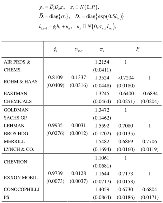
Table 6: MCL Estimates for One-Block Trivariate SV Models





 













, 1 , , 0, ,

diag , diag exp 0.5

, 0, , i it i it t t i i i it it i t i it it it u ii m y D D N P D D h h h u u N I            i  u ii, i Pi AIR PRDS.& CHEMS. 1.2154 (0.0411) 1

ROHM & HAAS 1.3524

(0.0448) -0.7204 (0.0180) 1 EASTMAN CHEMICALS 0.8109 (0.0409) 0.1337 (0.0316) 1.3245 (0.0464) -0.6400 (0.0251) -0.6894 (0.0204) GOLDMAN SACHS GP. 1.3472 (0.1462) 1 LEHMAN BROS.HDG. 1.5592 (0.1702) 0.7080 (0.0135) 1 MERRILL LYNCH & CO.

0.9935 (0.0276) 0.0031 (0.0012) 1.5482 (0.1694) 0.6869 (0.0160) 0.7706 (0.0119) CHEVRON 1.1061 (0.0681) 1 EXXON MOBIL 1.1644 (0.0717) 0.7173 (0.0153) 1 CONOCOPHILLI PS 0.9739 (0.0073) 0.0128 (0.0037) 1.4059 (0.0864) 0.6730 (0.0186) 0.6804 (0.0171) Note: Standard errors are given in parentheses.

Table 7: AIC and BIC for One-Component Trivariate SV Models

Chemicals General Financials Oil and Gas Producers LogLike -8875.86 -8545.33 -8454.49

AIC 17767.7 17106.7 16925.0

Table 8: MCL Estimates for BS-MSV Models (General Financials, Oil and Gas Producers)





 

















1 1 , 0, ,

diag , diag exp 0.5 ,

, 0, , diag , , , . t t t t t t t t t t B M u M y DD N P D D h h h N I I                    _       u GOLDMAN SACHS GP. LEHMAN BROS.HDG. MERRILL LYNCH & CO.

0.9961 (0.0021) 0.0020 (0.0009) CHEVRON EXXON MOBIL CONOCOPHILLIPS 0.9760 (0.0067) 0.0019 (0.0009) 0.0115 (0.0033)  _P GOLDMAN SACHS GP. 1.3506 (0.1971) 1 LEHMAN BROS.HDG. 1.5623 (0.2286) 0.7081 (0.0135) 1 MERRILL LYNCH & CO.

1.5797 (0.2338) 0.6796 (0.0163) 0.7690 (0.0120) 1 CHEVRON 1.1179 (0.0708) -0.4462 (0.0412) -0.4553 (0.0399) -0.4012 (0.0471) 1 EXXON MOBIL 1.1799 (0.0748) -0.4161 (0.0429) -0.4280 (0.0419) -0.4194 (0.0371) 0.7163 (0.0152) 1 CONOCOPHILL IPS 1.4300 (0.0921) -0.4271 (0.0428) -0.4476 (0.0400) -0.4282 (0.0424) 0.6697 (0.0185) 0.6778 (0.0170) 1

LogLike AIC BIC -16939.6 33931.2 34066.9 Note: Standard errors are given in parentheses.

Table 9: MCL Estimates for BS-MSV Models (General Financials, Chemicals)





 

















1 1 , 0, ,

diag , diag exp 0.5 ,

, 0, , diag , , , . t t t t t t t t t t B M u M y DD N P D D h h h N I I                    _       u GOLDMAN SACHS GP. LEHMAN BROS.HDG. MERRILL LYNCH & CO.

0.9743 (0.0068)

0.0107 (0.0037)

AIR PRDS.& CHEMS. ROHM & HAAS

EASTMAN CHEMICALS 0.8817 (0.0334) 0.0204 (0.0056) 0.0867 (0.0258)  _P GOLDMAN SACHS GP. 1.3086 (0.1789) 1 LEHMAN BROS.HDG. 1.5036 (0.0954) 0.7076 (0.0158) 1 MERRILL LYNCH & CO.

1.4683 (0.2354) 0.6871 (0.0182) 0.7639 (0.0162) 1 AIR PRDS.& CHEMS. 1.2232 (0.1017) -0.5114 (0.0343) -0.5390 (0.0361) -0.5463 (0.0335) 1

ROHM & HAAS 1.3680 (0.0519) -0.4351 (0.0433) -0.4602 (0.0632) -0.5118 (0.0492) -0.7109 (0.0172) 1 EASTMAN CHEMICALS 1.3464 (0.0512) -0.4236 (0.0495) -0.4675 (0.0770) -0.3970 (0.0551) -0.6219 (0.0243) -0.6810 (0.0208) 1

LogLike AIC BIC -17311.2 34674.5 34810.2 Note: Standard errors are given in parentheses.

Table 10: MCL Estimates for BS-MSV Models (Oil and Gas Producers, Chemicals)





 

















1 1 , 0, ,

diag , diag exp 0.5 ,

, 0, , diag , , , . t t t t t t t t t t B M u M y DD N P D D h h h N I I                    _       u CHEVRON EXXON MOBIL CONOCOPHILLIPS 0.9597 (0.0101) 0.0178 (0.0051)

AIR PRDS.& CHEMS. ROHM & HAAS

EASTMAN CHEMICALS 0.8413 (0.0353) 0.0150 (0.0054) 0.1080 (0.0261)  _P CHEVRON 1.1108 (0.0555) 1 EXXON MOBIL 1.1688 (0.0595) 0.7245 (0.0154) 1 CONOCOPHILL IPS 1.4075 (0.0734) 0.6777 (0.0191) 0.6883 (0.0174) 1 AIR PRDS.& CHEMS. 1.2169 (0.0436) -0.3623 (0.0687) -0.4741 (0.0409) -0.4139 (0.0478) 1

ROHM & HAAS 1.3572 (0.0190) -0.5088 (0.0365) -0.4591 (0.0386) -0.4648 (0.0375) -0.7127 (0.0177) 1 EASTMAN CHEMICALS 1.3285 (0.0477) -0.3989 (0.0520) -0.4789 (0.0396) -0.3859 (0.0551) -0.6237 (0.0252) -0.6810 (0.0207) 1

LogLike AIC BIC -17260.4 34572.7 34708.4 Note: Standard errors are given in parentheses.

Table 11: MCL Estimates for BS-MSV Models (General Financials, Oil and Gas Producers, Chemicals)





 

















1 1 , 0, ,

diag , diag exp 0.5 ,

, 0, , diag , , , . t t t t t t t t t t B M u M y DD N P D D h h h N I I                           _u GOLDMAN SACHS GP. LEHMAN BROS.HDG. MERRILL LYNCH & CO.

0.9873 (0.0058) 0.0043 (0.0012) CHEVRON EXXON MOBIL CONOCOPHILLIPS 0.9618 (0.0094) 0.0019 (0.0012) 0.0171 (0.0049)

AIR PRDS.& CHEMS. ROHM & HAAS

EASTMAN CHEMICALS 0.8598 (0.0489) 0.0096 (0.0040) 0.0143 (0.0052) 0.0902 (0.0326)

LogLike AIC BIC -25660.0 51428.0 51709.8