Weakly Supervised Learning Algorithms and an Application to Electromyography

(1)

Weakly Supervised Learning Algorithms

and an Application to Electromyography

by

Tameem Adel Hesham

A thesis

presented to the University of Waterloo in fulfillment of the

thesis requirement for the degree of Doctor of Philosophy

in

Systems Design Engineering

Waterloo, Ontario, Canada, 2014

c

(2)

Author’s Declaration

I hereby declare that I am the sole author of this thesis. This is a true copy of the thesis, including any required final revisions, as accepted by my examiners.

(3)

Abstract

In the standard machine learning framework, training data is assumed to be fully supervised. However, collecting fully labelled data is not always easy. Due to cost, time, effort or other types of constraints, requiring the whole data to be labelled can be difficult in many applica-tions, whereas collecting unlabelled data can be relatively easy. Therefore, paradigms that enable learning from unlabelled and/or partially labelled data have been growing recently in machine learning. The focus of this thesis is to provide algorithms that enable weakly annotating unlabelled parts of data not provided in the standard supervised setting consist-ing of an instance-label pair for each sample, then learnconsist-ing from weakly as well as strongly labelled data. More specifically, the bulk of the thesis aims at finding solutions for data that come in the form of bags or groups of instances where available information about the labels is at the bag level only. This is the form of the electromyographic (EMG) data, which represent the main application of the thesis. Electromyographic (EMG) data can be used to diagnose muscles as either normal or suffering from a neuromuscular disease. Muscles can be classified into one of three labels; normal, myopathic or neurogenic. Each muscle consists of motor units (MUs). Equivalently, an EMG signal detected from a muscle consists of motor unit potential trains (MUPTs). This data is an example of partially labelled data where instances (MUs) are grouped in bags (muscles) and labels are provided for bags but not for instances.

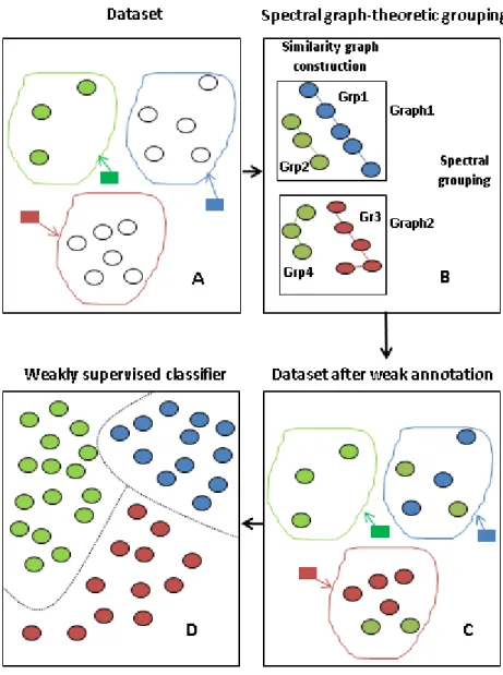
First, we introduce and investigate a weakly supervised learning paradigm that aims at improving classification performance by using a spectral graph-theoretic approach to weakly annotate unlabelled instances before classification. The spectral graph-theoretic phase of this paradigm groups unlabelled data instances using similarity graph models. Two new similarity graph models are introduced as well in this paradigm. This paradigm improves overall bag accuracy for EMG datasets.

Second, generative modelling approaches for multiple-instance learning (MIL) are presented. We introduce and analyse a variety of model structures and components of these generative models and believe it can serve as a methodological guide to other MIL tasks of similar

(4)

form. This approach improves overall bag accuracy, especially for low-dimensional bags-of-instances datasets like EMG datasets.

MIL generative models provide an example of models where probability distributions need to be represented compactly and efficiently, especially when number of variables of a certain model is large. Sum-product networks (SPNs) represent a relatively new class of deep probabilistic models that aims at providing a compact and tractable representation of a probability distribution. SPNs are used to model the joint distribution of instance features in the MIL generative models. An SPN whose structure is learnt by a structure learning algorithm introduced in this thesis leads to improved bag accuracy for higher-dimensional datasets.

(5)

Acknowledgements

I would like to thank my supervisors Dr. Ali Ghodsi and Dr. Dan Stashuk. Dr. Ghodsi’s knowledge, of which I failed to know the limits, was a great incentive for me to understand how important it is to be aware of not only one specific area of research but also related areas. The insightful discussions I had with him have provided me with guidance and inspiration. Also, Dr. Ghodsi’s probabilistic graphical models course was the beginning of an obsession for me.

I am grateful to Dr. Alex Wong. In addition to his important feedback on my thesis, it has been great working with him. His impressive sharpness and profound understanding of both the core and the application side of my thesis, have been invaluable for the progress of this work.

It has been pleasure working with Dr. Dan Lizotte. His broad and deep knowledge as well as his support have kept my enthusiasm alive throughout the thesis.

I would also like to thank the other members of my PhD committee Dr. Marco Valtorta and Dr. Paul Fieguth for their valuable comments and feedback on my thesis.

(6)

List of Figures

1.1 Four learning paradigms . . . 2

1.2 Neuromuscular Disorders and the Corresponding MUPs . . . 4

1.3 A schematic representation of the main data and paradigms in use . . . 5

2.1 A motor unit . . . 22

2.2 Normal MU versus Myopathic and Neurogenic MUs . . . 25

2.3 Examples of healthy, Neuro and Myo EMG signals. . . 25

3.1 3-Class partially labelled data of the bags-of-instances setting . . . 34

4.1 A schematic representation of the main steps of the introduced weakly super-vised paradigm . . . 40

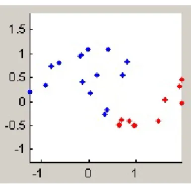
4.2 DatasetA: A toy dataset . . . 44

4.3 Similarity graph ofDatasetA as a result of applying anϵ-neighbourhood graph 45 4.4 Similarity graph of DatasetA as a result of applying a symmetric k-nearest neighbour graph . . . 46

4.5 Similarity graph ofDatasetAas a result of applying a mutualk-nearest neigh-bour graph. . . 47

4.6 Similarity graph of DatasetAas a result of applying a probabilistic threshold similarity graph with w= 0.073 . . . 47

4.7 F-measure values for datasets with ground truth labels . . . 56

4.8 Davies-Bouldin index values for datasets without ground truth labels . . . . 57

5.1 The BIF model structure . . . 65

5.2 Average LOI vs. Turns . . . 81

5.3 Average LOI vs. Amplitude . . . 81

5.4 Average LOI vs. Area. . . 82

5.5 Average LOI vs. Thickness . . . 82

5.6 Average LOI vs. Turns and Amplitude . . . 83

5.7 Average LOI vs. Amplitude and Area . . . 83

5.8 Average LOI vs. Area and Thickness . . . 84

(11)

(12)

List of Tables

3.1 EMG Feature descriptions. . . 35

4.1 Clustering indices values based on different similarity graph models. . . 55

4.2 Muscle classification accuracy based on the proposed weakly supervised clas-sifiers vs. a fully supervised classifier. . . 59

5.1 Results of the EMG datasets . . . 78

5.2 Results of the EMG datasets with the BIF structure using different initial values of P(I|B). . . 78

5.3 Results of the MUSK dataset . . . 79

5.4 Comparison between the generative MIL model BIF and weakly supervised learning paradigm on the EMG datasets . . . 80

6.1 SPN-Gens on an Example Data Matrix . . . 98

6.2 SPN-R1DBiclus on the Same Data Matrix . . . 100

(13)

Abbreviations

CDSS Clinical Decision Support System CPT Conditional Probability Table EMG ElectroMyoGraphy

i.i.d. Independent and Identically Distributed IRB InstitutionalReview Board

KDE Kernel Density Estimation LDA Linear Discriminant Analysis LOI Level Of Involvement

MIL Multiple-InstanceLearning MLE Maximum-Likelihood Estimation MU Motor Unit

MUP Motor Unit Potential MUPT Motor Unit Potential Train NMF Nonnegative MatrixFactorization PDF Probability Density Function QDA Quadratic Discriminant Analysis R1D Rank-One Downdate

(14)

Chapter 1

Introduction

Two of the most eminent and contrasting statistical machine learning paradigms are super-vised and unsupersuper-vised learning. In supersuper-vised learning (sometimes referred to as learning with a teacher), a learner is given data samples/instances where each instance has its own label and the task of the learner is to implement training on these labelled instances so that previously unseen or test instances can be reliably labelled by the developed learning model [Hastie et al., 2009]. In unsupervised learning, a learner is given unlabelled data in-stances and the task is to derive a descriptive structure of the given unlabelled data [Hastie et al., 2009]. Nowadays, learning has numerous applications, like spam detection, speech recognition, text categorisation, handwritten digit recognition and many others.

There are other learning paradigms where learning is not fully supervised or, equivalently, where a learner is given non-perfect data for training. The goal of these paradigms is to learn a predictive model based on the available data. Then, test data are to be labelled using this model. Non-perfect (partially labelled) data can take different settings, each having its corresponding learning paradigm(s). The most common paradigm that learns from partially labelled data is semi-supervised learning, which aims at developing models by learning from partially labelled data consisting of labelled as well as unlabelled instances [Zhou and Xu,

2007]. In many problems, using unlabelled or weakly labelled instances in conjunction with labelled instances can lead to an improvement in the performance of the learning model compared to a model based on labelled instances only, and this is the premise on which

(15)

(a) Supervised Learning (b) Unsupervised Learning

(c) Semi-supervised Learning (d) Bags-of-Instances. Each bag has a label

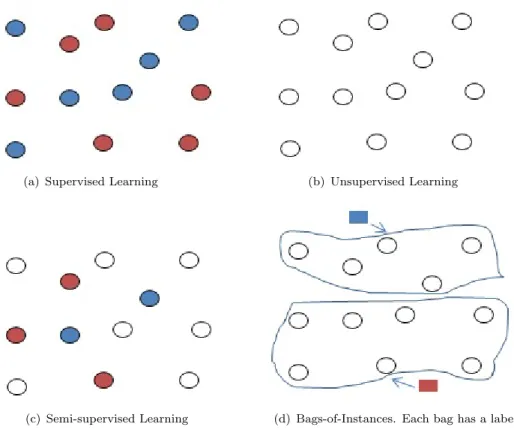
Figure 1.1: Data settings for four Learning Paradigms. (a)Supervised Learning: all instances are

labelled. (b)Unsupervised Learning: all instances are unlabelled. (c)Semi-supervised Learning: some instances are labelled and some are unlabelled. (d) Bags-of-Instances Learning: Only bags

are labelled.

semi-supervised learning is based. The number of unlabelled instances is usually greater than the number of labelled instances in paradigms of this kind. This is a consequence of the relative ease by which unlabelled data can be obtained in numerous applications. Semi-supervised learning is commonly considered a subset paradigm of weakly supervised learning [Joulin and Bach, 2012, Li et al., 2013, Guo et al., 2011] but due to its increasing importance, it is also considered by some (like Guillaumin et al. [2010]) as a related but separate paradigm. Weakly supervised learning generalises other learning paradigms, like paradigms acting on settings where data is given in the form of bags or groups of instances and label information is given at the bag level only. Figure 1.1 depicts the difference between supervised, unsupervised, semi-supervised and bags-of-instances weakly supervised learning. The focus of this thesis is on paradigms where learning is applied on bags of instances. Label information in this case is provided at the bag level only and the introduced algorithms aim

(16)

at, first weakly annotating data at the instance level, then applying weakly supervised learning on the resulting weakly labelled data. We are mainly concerned with the bags-of-instances setting but depending on each introduced solution, a subproblem can be cast to another setting and in order to demonstrate the validity of the solution to the subproblem, we may check another data setting that corresponds to the subproblem.

A common example of the bags-of-instances setting is an object recognition image database with binary labels where a positive bag label indicates the existence of a specific object in the corresponding image whereas a negative bag label means that the object does not exist [Blaschko et al., 2010,Bergamo and Torresani,2010]. A negative labelled image in this case is fully labelled. A positive labelled image can be fully labelled if the exact location(s) of the object is identified, but more often than not this is not the case and positive labelled images are partially labelled each with a latent variable referring to the location of the object in the image.

The main application of the research in this thesis is a muscle classification problem based on electromyographic (EMG) data. EMG muscle data represent partially labelled data where labels are available only at the bag level. Electromyographic (EMG) signals provide a unique insight into both the structure and function of muscles [Farkas et al.,2010] and can therefore be used in a muscle classification problem whose practical aim is muscle diagnosis. An EMG signal of a muscle consists of motor unit potential trains (MUPTs) whereas each MUPT represents the activity of a motor unit (MU) during a muscle contraction. Motor units (MUs) are components of a muscle. Motor unit (MU) activation changes caused by a disorder are reflected in the characteristics of EMG signals allowing them to be used to help diagnose neuromuscular disorders. As shown in the right hand side of Figure 1.2, EMG signals representing the electrical activities of MUs have different characteristics depending on whether the MU is normal, myopathic or neurogenic. More details about the morpholog-ical changes in muscles due to neuromuscular disorders are provided in Chapter 2. In EMG datasets, MU labels are based on the label of the muscle from which they were detected and do not consider the actual clinical state of the MU. Therefore, EMG datasets are partially labelled data where labels are provided for the bags but not for individual instances.

(17)

Figure 1.2: Schematic representation of the effects of the various categories of neuromuscular disorders [Farkas et al., 2010]. A Normal motor unit (MU), B Neurogenic (MU) & C Myopathic

(MU). In the right hand side, motor unit potentials (MUPs) of each label are displayed.

The primary goal of the research in this thesis is to provide bag (muscle) accuracy for the muscle classification problem as well as bag accuracy for similar datasets that share the same bags-of-instances setting but might differ in the assumptions induced by the problem as well as size and dimension of the data.

The main problem therefore is to assign bag labels to data on the bags-of-instances form. There are subproblems as well. In the weakly supervised learning paradigm, there is a grouping subproblem whose solution is tested on other unlabelled datasets. In the genera-tive multiple-instance learning (MIL) modelling paradigm, representing feature probability distributions efficiently is another subproblem. One subproblem that is related to the EMG data only is to get a measure of confidence in muscle characterisations and another of level of involvement (LOI) of motor unit potentials of a muscle.

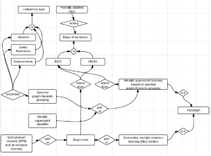
Figure 1.3 provides a schematic description of the data and paradigms introduced to learn from them.

(18)

Figure 1.3: A representation of data and paradigms in use. EMG datasets are the main datasets in use but there are other datasets, like the MUSK dataset. Both these datasets are bags-of-instances datasets. Other datasets in use, for a subproblem related to one of the paradigms, are Abalone, Swiss Banknotes and Segmentation. The latter three datasets are unlabelled. The first introduced paradigm is a weakly supervised learning paradigm based on spectral graph-theoretic grouping. It is applied on the EMG datasets. It is not applied on the MUSK data because it is not applicable on the first phase of the paradigm which is the spectral graph-theoretic grouping phase. The spectral graph-theoretic grouping phase aims at weakly annotating unlabelled data by first grouping them then assign a label to each group based on the relationship between labelled and unlabelled data. This means that the first step of the spectral graph-theoretic grouping phase is a grouping process. The grouping process is one of the subproblems and this phase on its own is tested on unlabelled datasets; Abalone, Swiss Banknotes and Segmentation. The second phase of the weakly supervised learning paradigm is the weakly supervised classifier used to classify EMG data. The second introduced paradigm is the generative MIL modelling paradigm. In this paradigm, generative models are constructed by Bayes nets. It is applied on both EMG and MUSK datasets. One subproblem of this paradigm is to represent feature probability distributions especially for medium or large dimensional datasets, like the MUSK dataset. Sum Product networks (SPNs) is a model by which probability distributions can be represented efficiently. SPNs are applied as a part of the

(19)

1.1 Contributions

Each contribution out of the first three contributions represents a strategy or part of a strategy that learns from data of the bags-of-instances setting. We outline these strategies identifying the main characteristics of each.

Weakly Supervised Learning based on Spectral Graph-Theoretic Grouping In this weakly supervised learning paradigm, a learner receives a training set containing fully labelled bags of instances as well as partially labelled bags of instances. First, a spectral graph-theoretic grouping phase is applied to weakly annotate unlabelled data. Then a weakly supervised classifier is applied on weakly annotated data as well as labelled data. In the first phase, novel similarity graph models are proposed. Results show that the introduced spectral graph-theoretic approach is effective at weakly annotating unlabelled parts of the data, which results in an improved accuracy of the resulting weakly supervised classifier. This weakly supervised paradigm leads to an improved muscle classification accuracy. The spectral graph-theoretic grouping phase weakly annotates instances of the data, which are instances belonging to bags with known bag labels but unknown instance labels. This leads to the fact it can be used as an unsupervised learning approach because these instances it weakly annotates are unlabelled. Experiments are performed on some benchmark unla-belled datasets and results show that the introduced strategy is effective at constructing a descriptive grouping structure of each of these datasets.

Generative Multiple-Instance Learning (MIL) Models

In its original setting introduced byDietterich et al.[1997], multiple-instance learning (MIL) referred to a binary class learning paradigm where instances are grouped into bags and a bag is considered positive if it contains at least one positive instance, otherwise a bag is labelled negative. We extend the definition of MIL to cover multi-class problems, introduce an MIL paradigm based on generative models and provide intuition and guidelines for applying these

(20)

generative models to MIL problems. A state-of-the-art solution to the problem of muscle classification is provided via the MIL paradigm.

Structure Learning of Sum-Product Networks (SPN)

Features used in the EMG data are 8 features. For bags-of-instances datasets with a much greater number of features, MIL generative models perform relatively well but less well than they do with EMG datasets. Therefore, there is a need for a better way of handling the fea-ture dependence relationships in a more compact and tractable manner than those utilised in the MIL approach introduced above. The most commonly used MIL dataset in the litera-ture is referred to as the MUSK dataset [Dietterich et al.,1997] and it contains 168 features. Therefore, the MUSK dataset represents an example where there is a medium rather than small number of features and where the need to represent dependence relationships among features compactly and efficiently arises. Sum-product networks (SPNs) are probabilistic graphical models that are capable of providing deep architectures that can compactly rep-resent complex dependence relationships among variables while still remaining tractable. A new algorithm for learning the structure of SPNs is introduced and applied on the MUSK dataset. The constructed SPN extends the MIL generative models and bag accuracy results demonstrate that it better expresses dependence relationships.

Regarding the application, the contribution is providing state-of-the-art solutions to the muscle classification problem using both the weakly supervised learning paradigm and gen-erative MIL modelling paradigm on one of the two EMG datasets (upper leg) and using the generative MIL modelling paradigm on the other EMG dataset (lower leg). Also, the bag accuracy of the MUSK dataset that resulted from using SPNs to model instance feature distributions is near state-of-the-art results on the MUSK data.

(21)

1.2 Outline

Chapter 2 introduces background material related to the research of the thesis. It contains basic background material about statistical learning as well as unsupervised learning per-formed on undirected graphs. It also contains background about EMG data. In Chapter 3, the problem is formally defined along with a description of the bags-of-instances partially labelled data of interest. In Chapter 4, the weakly supervised learning paradigm is pre-sented. Chapters 5 and 6 are related to the generative MIL modelling paradigm. Chapter 5 presents the generative MIL models and their results on EMG and MUSK data. Chapter 6 presents the sum-product network (SPN) structure learning algorithm and how it leads to better results on the MUSK dataset when the respective SPN is used to model the instance feature distributions. Finally, concluding comments are given in Chapter 7. Chapters 4, 5 and 6 represent the chapters where the methodology as well as the contributions are. These 3 chapters begin with an overview each then a brief listing of the related work, followed by a description of the introduced algorithm and then the results.

The content of this thesis is mainly based on three publications. The weakly supervised learning paradigm is presented in Adel et al.[2014]. The work on MIL generative models is presented in Adel et al. [2013]. Finally the SPN structure learning algorithm, along with a more comprehensive set of experiments, is presented in Adel and Ghodsi [2014].

Other publications that were developed during the time of the thesis but are secondary to this document, include Adel et al. [2012] and Parsaei et al. [2012].

(22)

Chapter 2

Background

Here we present fundamental concepts that are used throughout this thesis. We start with a brief introduction of basic probability rules, then we follow with an overview about statistical learning and finally unsupervised learning performed on undirected graphs. The material in these sections is not comprehensive as it is presented with an eye on its use in the rest of the chapters of the thesis. Finally Section 2.4 presents information about EMG data, which represent the main application of the introduced paradigms.

2.1 Probability and Bayes Rule

A random variable is a variable whose value is not deterministic as it is subject to variability due to randomness [Yates et al., 2003]. A random variable can be assigned a value out of a set of possible values. Confidence that a random variable X has a specific value is denoted by its probability p(x), i.e. 0≤p(x)≤1. Note that, as a convention, we denote realisations of random variables in lower case. The function describing the set of values of a random variable and their respective probabilities is referred to as a probability distribution p(X). If the set of possible values X can take is countable, then the probability distribution is a probability mass function (PMF), whereas an uncountable set of values within one or more intervals is represented by a probability density function (PDF). The probability that a random variable Y is equal to a certain value given that another random variable X

(23)

is definitely equal to another value, is known as the conditional probability p(y|x). The probability that two random variables X &Y are equal to two respective values is referred to as the joint probability p(x, y). Similar to p(X), p(Y|X) and p(X, Y) can be cast as probability distributions by normalisation. If the probability distributions of p(X, Y) and p(X) are known, then p(Y|X) can be obtained as follows:

p(Y|X) = p(X, Y)

p(X) (2.1)

As p(X|Y) can be obtained similarly, Bayes rule can now be presented as follows:

p(Y|X) = p(X|Y)p(Y)

p(X) (2.2)

2.2 Statistical Learning

In Chapter 1, we briefly presented a high-level taxonomy of learning paradigms that was mainly based on the setting of the data available for learning. Here we present an example followed by a more formal notion of statistical learning.

Imagine you are given a set of N musical tunes each with its music genre. You are assigned the task of assigning music genres to another set of songs or musical tunes. The latter set of tunes need to be labelled each by one genre. You want to complete the task properly by minimising the number of tunes you ultimately classify incorrectly, out of those in the set. You also want to finish the task as soon as you can, provided that you still do it properly; which means that if you can assign the correct genre to a tune in its first few seconds, this is better than doing the same after two minutes. You decide which tune belongs to which genre, based on the experience you obtained by listening to the N labelled tunes and based on the group of genres from which you pick one for each tune. Your brain chooses features of the tune that are relevant to the genre assigning task at hand. For example, if tunes are to be classified into “classical” or “rock” tunes, your criterion can heavily count on assigning one of the two genres based on whether or not there is singing, not only music. However, if the

(24)

group of genres include “folk” as well, you should add tune features that are relevant to the genres, or more precisely, relevant to the difference between a genre and another. Features like time signature and whether or not there are electrical instruments could be used to differentiate “rock” from “folk”. Further features should be added in case “alternative rock” (similar to “rock” in all the previously mentioned features) is added to the group of genres; e.g. lyrical style. As you are required to be accurate as well as time efficient, you try to base your genre assignment on features that are relevant to the discrimination among genres as well as non-redundant.

Learning problems of that kind can be represented by a statistical model. We start with describing a statistical learning model.

2.2.1 Statistical Learning Model

Input The learner receives a set of N independent and identically distributed (i.i.d.) instances where each instance X has p features and has a label Y assigned to it. The set of possible values of Y has a cardinality 1 _{equal to} _t_{. This set of instances is referred to}

as training instances Hastie et al. [2009]. Training data is assumed to be drawn from an unknown distribution.

Sticking to the above example. Input to the learner is a set of tunes, where each tune has

p features, e.g. instrumentation, time signature, energy, duration, tempo, etc. Each tune is also assigned a label indicating its genre.

Output The learner is required to build a prediction function that maps X to Y. The prediction function is used to predict an output ˆY of each instance belonging to another set of instances, referred to as the test set. The learner bases the mapping he develops from X

to Y on the training instances (supervised learning). In doing so, the learner uses features that he finds relevant to the mapping, i.e. features that provide useful information about the mapping, and non-redundant, i.e. each feature provides further useful information than the already selected features. When t is finite, the prediction function can be referred to as

1

(25)

a classifier. Assuming a Bayes classifier, t = 2 and Y ∈ {1,2}, if P(y= 1|x)> P(y= 2|x), then ˆy= 1, and vice versa.

This is the task of assigning genres to each test tune in our example.

A prediction function usually contains parameters β. In case a prediction function fits the training instances too well, there is a risk of overfitting. Overfitting refers to the phenomenon of a classifier that performs accurately on training data but fails to generalise and does not perform well on other data instances. In order to avoid overfitting,βshould be chosen so that a classifier has a good balance between its bias and variance. Bias refers to the accuracy of a classifier on the training data instances whereas variance refers to the sensitivity of a classifier to changes in the set of training instances [Geman et al., 1992]. Classifiers that overfit have high variance. The bias-variance tradeoff (also referred to as bias-variance dilemma) has been well studied in machine learning. For example,Hastie et al.[2009],James et al.[2013],

Geman et al. [1992] present more comprehensive material on this subject.

Overfitting can be thought of as if you try too hard to adjust your criterion of deciding a genre of a tune based on very specific characteristics of each tune you had in the training set (low bias and high variance) rather than having a better sense of what generally discriminates a genre from another and what is a special characteristic of few training tunes (higher bias and lower variance).

There is more than one measure by which the performance of a classifier can be evaluated. One of them is error rate. Error rate is defined the probability of a misclassification. It is equal to the number of misclassified test instances divided by the total number of test instances. Bayes optimal error rate is defined as the error achieved by an optimal classifier and it represents the theoretical minimum error on a certain dataset [Keinosuke, 1990]. The Bayes optimal error rate is theoretical mainly because the distribution from which the training (and test, assuming they both were drawn from the same distribution) data is drawn, is unknown. Accuracy of a classifier is equal to 1− error rate, which is equal to the number of correctly classified test instances divided by the total number of test instances.

(26)

Least Squares To build a classifier, its parameters β should be chosen according to a criterion. One criterion aims at minimising the residual sum of squares of errors committed in classifying test instances. This criterion is referred to as least squares. Assuming that

fβ(x) is the classifier’s output for an instance x, least squares can be formulated as follows [Hastie et al., 2009]:

minimise least squares(β) = N

∑

i=1

(yi−fβ(xi))2 (2.3) Maximum Likelihood Another criterion, which is based on likelihood, is referred to as maximum likelihood estimation (MLE). Let’s first describe the likelihood. Likelihood is a function of the parameters β of a classifier, or more generally of a statistical model. It represents the probability that training instances are equal to their respective values given the parameter values. Likelihood of a classifier can be described as l(β) = p(Y, X|β). According to maximum likelihood, optimal values of the parameters β are those that make the probability of the observed training samples as large as possible [Hastie et al., 2009]. Because it is more convenient to work with logarithms and they do not change values of β

that maximise the likelihood, log-likelihood is usually used rather than likelihood.

Generative Models and Discriminative Models Describing the likelihood function as

l(β) = p(Y, X|β) refers to a generative model where the goal is to learn a joint distribu-tion that underlies the data X as well as the unobserved variable Y that represents their labels. In contrast with generative models, the likelihood function of a discriminative model would be equal to l(β) = p(Y|X, β) because discriminative models model the conditional probability distribution of an unobserved variable Y given observed data represented by

X. One advantage of generative models versus discriminative models is that they can be used in data simulation because they model both the data and the label or unobserved variable. Generative models can also be used in classification because, the joint distribution they provide can be used in classification by applying Bayes rule. On the other hand, dis-criminative models can sometimes lead to better classification performance than generative

(27)

models [Lafferty et al., 2001, Ng and Jordan, 2001], but this depends on the problem and the data. Discriminative models usually perform well when there is plenty of labelled data, but typically do not exploit unlabelled data. In contrast, generative models can make use of unlabelled data in learning via a latent variable model [Bishop and Lasserre, 2007]. Ng and Jordan[2001] reached an important conclusion, related to the asymptotic error of both models when used as classifiers. They noted that while the asymptotic error is lower with dis-criminative classifiers, generative classifiers reach their asymptotic error much more quickly. A generative classifier can be considered a density estimation problem where it is required to estimate the probability distribution P(X, Y). Similarly, a discriminative classifier can be considered a density estimation problem but the probability distribution to be estimated is P(Y|X) [Hastie et al., 2009]. Examples of generative classifiers are linear discriminant analysis (LDA) and Naive Bayes (NB), while examples of discriminative classifiers include logistic regression and support vector machines (SVM).

Inductive Bias Inductive bias refers to the set of assumptions the learner strictly follows to build the learning function or classifier in our case. Each assumption represents a restriction on the available function space on which the learner builds the learning function, [Ben-David et al., 2011]. One example of an inductive bias is to minimise the number of parameters β

in the above generative classifier. This comes as a result of Occam’s Razor which favours the simplest consistent rule. One of the benefits of Occam’s Razor is that the simplest rule (having minimum number of parameters in our case) can lead to better generalisation, which eventually turns into smaller variance values [Domingos,1999]. One further advantage of generative models versus discriminative models, as will be explained in more detail in Chapter 5, is that they allow for expert domain knowledge to be incorporated into the model in a straightforward manner, leading to good inductive bias.

2.3 Unsupervised Learning on Undirected Graphs

Back to the example of musical tunes defined in Section 2.2. Imagine you are not given any labelled tunes to prepare a criterion. You are given a set of tunes without genres assigned

(28)

to them and are required to provide some summarising or descriptive information of the set. As a starting point, your brain will start looking for major similarities and dissimilarities among the tunes so that you can start providing the required information.

More formally, in unsupervised learning, the learner is given a setXconsisting ofN instances

x1, x2, ..., xN without labels. The task of the learner is to process the data so that a specific form of descriptive statistics about it is obtained. One common form of such statistics is clustering. We focus here on clustering as it is the single approach of unsupervised learning that is targeted in this thesis. Therefore let’s describe clustering as follows:

Clustering Input The learner receives a set X of N i.i.d. instances where each instance has p features. Even if it is not always the case, let’s assume another number k is given, representing the number of clusters. This is inline with the research in this thesis.

Clustering Output The learner is required to return a partition of theN instances intok

disjoint subsetsC1, C2, ..., Ck, where

∪k

i=1Ci =X[Ben-David et al.,2006]. A good

partition-ing should minimise pairwise distances among instances of the same subset and maximise pairwise distances among instances of different subsets, so that subsets are homogeneous and well separated, respectively.

Here the focus is on clustering on undirected graphs. We proceed with some related defini-tions.

Similarity Graphs Assume the similarity between each pair of instances xi and xj in X, is indicated bysij ≥0. Data instances can be represented by a graphG= (V, E) where each data instance xi is represented by a vertex vi. The decision whether or not to connect two vertices by an edge, depends on the similarity sij between the corresponding two instances. If sij is larger than a certain threshold (indicated by the similarity graph model followed), then the two vertices are connected by an edge whose weight is sij [von Luxburg, 2007], otherwise the two vertices are not connected. Therefore, for any elementwij of the weighted adjacency matrix W, wij ≥0.

(29)

The degree of a vertex vi is di = N ∑ j=1 wij (2.4)

The degree matrix D is a diagonal matrix, whose elements are the vertex degrees. For a subset A, A⊂V, size of A can be defined as:

|A|= number of vertices in A (2.5) or

vol(A) =∑ i∈A

di (2.6)

The complement of a subset A is denoted by ¯A. For any two subsets A and B, A, B ⊂V, define:

W(A, B) = ∑ i∈A,j∈B

wij (2.7)

In Section 4.2, a description of the most commonly used similarity graph models is provided. Based on the graph representation of instances, clustering can be formulated as follows: Graph Clustering The learner is required to return a partition of the graph into disjoint subsets, or groups of vertices, where edges between vertices of the same group have weights that are as high as possible (homogeneous groups) and edges between vertices of different groups have weights that are as low as possible (well separated groups).

Graph Cut The minimum cut (mincut) of a graph is a partition of the graph whose cut has the smallest possible sum of weights. For a partition consisting of k groups, mincut can be solved by choosing a partition C1, C2, ..., Ck such that the following is minimised [Stoer

and Wagner, 1997]: cut(C1, C2, ..., Ck) = 1 2 k ∑ i=1 W(Ci,C¯i) (2.8)

(30)

In order to prevent trivial solutions, e.g. one vertex groups, restrictions on the minimum size of a group are imposed. Two common objective functions, each related to one definition of a group size, are listed here. One is referred to as RatioCut [Hagen and Kahng, 1992]. The other objective function is referred to as Ncut [Shi and Malik,2000].

RatioCut(C1, C2, ..., Ck) = k ∑ i=1 cut(Ci,C¯i) |Ci| (2.9) N Cut(C1, C2, ..., Ck) = k ∑ i=1 cut(Ci,C¯i) vol(Ci) (2.10)

These updated forms turn the mincut problem into an NP hard problem. Spectral clustering can solve relaxed versions of both problems [von Luxburg,2007].

Before proceeding with a brief description of spectral clustering algorithms, graph Laplacian matrices are introduced first. Recall that D is the degree matrix and W is the weighted adjacency matrix. The unnormalized graph Laplacian is equal to the following:

L=D−W (2.11)

There are two ways by which a normalized graph Laplacian can be calculated, which are as follows: Lnor1 =D− 1 2LD− 1 2 (2.12) or Lnor2 =D−1L (2.13)

2.3.1 Spectral Clustering Algorithms

Algorithms of spectral clustering can be mainly divided into three algorithms, as per the graph Laplacian used [von Luxburg, 2007]. For each of them we assume an access to the following as an input.

(31)

Input A similarity matrix S ∈ RN×N _where _s

ij denotes similarity between xi and xj. Number of clusters k is also given.

Output ClustersC1, C2, ..., Ck where each instancexi belongs to one and only one cluster. Unnormalized Spectral Clustering

• Construct a similarity graph model by one of the algorithms described in Section 4.2 or one of the two introduced similarity graph models described throughout Chapter 4.

• Calculate the unnormalized Laplacian L=D−W.

• Calculate the first k eigenvectors ev1, ev2, ..., evk of L.

• LetEV ∈RN×k _{be a matrix where columns of}_EV _are _ev

1, ev2, ..., evk, and let yi ∈Rk be the ith row ofEV.

• Cluster yi, i= 1,2, ..., n into clusters C1, C2, ..., Ck using k-means. Normalized Spectral Clustering according to Shi and Malik [2000]

• Calculate the unnormalized Laplacian Lnor2 =D−W.

• Calculate the first k generalised eigenvectors ev1, ev2, ..., evk of the generalised eigen-value problem Lnor2 ev=γ D ev.

• LetEV ∈RN×k _{be a matrix where columns of}_EV _are _ev

1, ev2, ..., evk, and let yi ∈Rk be the ith row ofEV.

• Cluster yi, i= 1,2, ..., n into clusters C1, C2, ..., Ck using k-means. Normalized Spectral Clustering according to Ng et al. [2002]

(32)

• Calculate the normalized Laplacian Lnor1 =D− 1 2LD−

1 2. • Calculate the first k eigenvectors ev1, ev2, ..., evk of Lnor1. • Let EV ∈RN×k _{be a matrix where columns of} _EV _are _ev

1, ev2, ..., evk. • Construct a matrix T ∈ RN×k, tij = evij/( ∑ kev 2 ik) 1

2, which represents rows of EV

normalized to norm 1. Let yi ∈Rk be the ith row of T.

(33)

2.4 EMG Background

In the previous sections, we presented information about the learning techniques that will be used in the algorithms by which the problems are to be solved. Here we give an overview of the EMG data which represent the main application. As the subject is not so common, we give more detailed information in this section than what is required for the introduced paradigms, so that it is easier to understand the whole EMG process.

Human muscles are composed of motor units and each motor (MU) unit is composed of a specific α-motor neuron and the muscle fibres it innervates. A motor neuron innervates the muscle fibres of an MU via the neuromuscular junction (NMJ) formed at the terminal end of each branch of its axon. Voluntary muscle contractions are initiated when the central nervous system recruits MUs by activating their motor neurons, which in turn, via their NMJs, activate their muscle fibres. At each NMJ, a region of transmembrane current is produced across the sarcolemma membrane of its corresponding fibre when the motor neuron is activated (i.e. discharges an action potential). This transmembrane current creates a change in transmembrane potential (or action potential) which propagates along the fibre and initiates/co-ordinates its contraction [Campbell and Reece,2001]. The currents creating the action potentials of the activated fibres of recruited MUs summate to create dynamic electric fields in the volume conductor in and around muscles. Electrodes placed in these electric fields detect time changing voltage signals which are the electromyographic (EMG) signals discussed in this section. When a muscle is affected by a neuromuscular disorder, characteristics of its action potentials, and as a result of the EMG signals they create, change depending on whether the muscle is affected by a myopathic or neurogenic disorder and the extent to which the muscle is affected. Therefore, quantitative EMG signal analysis can be used to support the diagnosis of neuromuscular disorders. Clinical quantitative electromyography (QEMG) attempts to use the information contained in an EMG signal to classify the muscle from which it was detected in order to support clinical decisions related to the diagnosis, treatment or management of neuromuscular disorders.

(34)

2.4.1 Muscle Morphology, Physiology and Electrophysiology 2.4.1.1 Morphological and Physiological Description of a Muscle MU Structure and Layout

Each muscle consists of muscle fibres. The muscle fibres of a muscle are grouped according to their innervatingα-motor neuron. An MU refers to a single α-motor neuron and the muscle fibres it innervates [Adel et al., 2012]. A voluntary muscle contraction is initiated by the activation of motor neurons whose axons propagate action potentials to their terminal ends where they join with a muscle fibre via a NMJ as shown in Figure 2.1. More specifically, a NMJ is the area where the axon terminal of a motor neuron axon innervates a muscle fibre. In a normal muscle, when a motor neuron is activated (i.e. discharges an action potential) each of its innervated muscle fibres are also activated via their respective NMJ. At each NMJ, following the arrival of the action potential at its axon nerve terminal, a region of transmembrane current is produced across the sarcolemma membrane of its corresponding fibre which creates a change in muscle fibre transmembrane potential (or a muscle fibre action potential) which propagates along the fibre and initiates/co-ordinates its contraction. Therefore, in normal muscle, activation of a motor neuron causes all of its innervated muscle fibres to contract and contribute to the force generated by the muscle.

For each muscle, there is a pool (or group) of motor neurons which are activated to produce a voluntary muscle contraction. The number of muscle fibres in a certain motor unit and the diameter of these fibres determine the size of the motor unit or the magnitude of its contribution to the muscle force created. The number of muscle fibres within a motor unit is not constant. Most muscles have large numbers of smaller MUs and smaller numbers of larger MUs.

An MU territory is the cross-sectional area of a muscle in which the fibres of an MU are randomly located. For a normal MU, its MU fibres are randomly positioned throughout its territory. MU territories can be conceived to be circular, with diameters taking values between 10 and 15 mm depending on the size of the MU. In addition, the MU territories of the MUs of a muscle are greatly overlapped. Therefore, in a normal muscle, adjacent muscle

(35)

Figure 2.1: A motor unit [Robergs and Roberts,1996].

fibres rarely belong to the same MU. Instead, the muscle fibres of an MU are interdigitated with muscle fibres of many other motor units.

MU Activation

When an MU is recruited, its motor neuron discharges a train of action potentials that propagate along its axon and, as described above, cause the muscle fibres of the MU to contract. The recruitment of only one MU leads to a weak muscle contraction. The recruit-ment of additional MUs leads to the activation of more muscle fibres and, as a result, muscle contraction becomes gradually stronger.

Motor unit recruitment or derecruitment refers to the activation or deactivation of an MU or population of MUs. Motor unit recruitment strategies vary depending on the inherent properties of the specific motor neuron pools of a muscle. Smaller muscles with smaller pools or numbers of MUs tend to recruit all of their MUs earlier during an increasing force contraction and often have all of their MUs recruited at 30% of maximal voluntary contraction. Larger muscles with large numbers of MUs recruit MUs throughout the entire range of force generation.

2.4.1.2 Muscle Electrophysiology

An innervated muscle fibre is activated when the currents created by the activity of its NMJ create a transmembrane action potential that then propagates in both directions along the muscle fibre away from the NMJ initiating and coordinating contraction of the fibre. In other

(36)

words, action potentials propagate along the axon of a motor neuron to activate the muscle fibres of an MU. The currents creating the action potentials of the activated muscle fibres linearly contribute to a spatially and temporally dynamic electric field created in the volume conductor in and around a muscle. The strength and spatial and temporal complexity of the created electric field is determined by the number of MUs active and their size. Electrodes placed in this electric field can be used to detect a time changing voltage signal (i.e. an EMG signal).

2.4.2 EMG Signals

2.4.2.1 Volume Conduction and Detection of EMG Signals

“Volume conduction is the spread of current from a potential source through a conducting medium, such as body tissues” [Dumitru et al.,2002]. Simulation models have been devised so that the effects of having different kinds of volume conductors and arrangements of detection electrodes on an EMG signal can be studied [Malmivuo and Plonsey, 1995].

2.4.3 Neuromuscular Disorders

Neuromuscular disorders change both the morphology and activation patterns of the MUs of the muscles affected. Therefore, the shapes of MUPs detected in muscles affected by neuromuscular disorders will differ from those detected in healthy or normal muscles. A normal muscle at rest will have no electrophysiological activity (i.e. there will be no electric field created in its surrounding volume conductor). Muscles affected by a neuromuscular disorder can have spontaneous muscle fibre activity called fibrillations and/or spontaneous MU activity called fasiculations.

Myopathic disorders cause muscle fibre atrophy, splitting, hypertrophy and necrosis. Exam-ples of atrophic and hypertrophic muscle fibres are diagrammed in Figure2.2. Atrophic and split muscle fibres have smaller diameters and slower muscle fibre action potential propaga-tion velocities. Therefore, they typically produce smaller and wider MFPs. Hypertrophic muscle fibres have larger diameters and faster muscle fibre action potential propagation ve-locities. They therefore produce in general large and narrower MFPs. Necrotic fibres are not

(37)

active and do not contribute to detected MUPs. As such, myopathic MUPs, in general, are composed of fewer MFP contributions of varying size and with larger temporal dispersion than in MUPs detected in normal muscles. Myopathic MUPs are therefore generally smaller in size and more complex than normal MUPs. The variation in muscle fibre action potential propagation velocity in a muscle fibre affected by a myopathic process can be greater than normal. This in turn can increase the instability of myopathic MUPs.

Because the MUs of a myopathic muscle are generally smaller during equivalent muscle activations more of them must be recruited and they need to be activated at higher firing rates compared to a normal muscle [Dumitru et al., 2002]. Therefore, at equivalent levels of muscle activation, EMG signals detected in a myopathic muscle can become more complex than EMG signals detected in a normal muscle (see Figure 2.3).

In contrast, neurogenic disorders cause the loss of MUs and muscle fibre denervation. Sub-sequently, the surviving MUs have increased numbers of fibres with greater spatial fibre densities relative to normal muscle as seen in Figure 2.2. The increased number of MU fibres results in MUPs comprised of larger numbers of MFP contributions. The greater spa-tial fibre densities result in grouped MFP contributions. Consequently neurogenic MUPs tend to be larger and more complex than normal MUPs sometimes with distinct components or phases (e.g. satellite potentials). During the acute phase of reinnervation newly formed NMJs have larger variations in the time taken to initiate a muscle fibre action potential in their respective muscle fibres. This results in increased instability of neurogenic MUPs. Because the MUs of a neurogenic muscle are generally larger and because they are fewer in number during equivalent muscle activations, fewer of them must be recruited but they need to be activated at higher firing rates compared to a normal muscle [Dumitru et al., 2002]. Therefore, at equivalent levels of muscle activation, EMG signals detected in a neurogenic muscle can become more complex than EMG signals detected in a normal muscle, as can be seen in Figure 2.3.

(38)

Figure 2.2: A. Normal MU vs. myopathic MU.

B. Normal MU vs. neurogenic MU [Barkhaus and Nandedkar,1994].

(39)

2.4.4 How to Extract Clinically Important Information

Suitably detected EMG signals contain information that can be used to assist with the diagnosis of neuromuscular disorders. Specific characteristics of a detected EMG signal can be related to the type of neuromuscular disorder present (i.e. myopathic or neurogenic) as well as the degree to which the muscle may be affected by a disorder. As described above, the changes in MU morphology and activation created by a disease process lead to expected changes in MUP shapes and stability as well as the level of EMG signal complexity. Specific aspects of the detected EMG signals can be analyzed to determine if they were most likely detected in a myopathic, normal or neurogenic muscle. This analysis can be qualitative or quantitative.

2.4.4.1 Qualitative Electromyography

One way of assessing the clinical state of a muscle is to qualitatively analyze EMG signals de-tected using needle electrodes following abrupt movement of the electrode, while the muscle is at rest and during low levels of muscle activation. Characteristics of the detected signals are subjectively compared to those expected to be detected in normal muscle. The signals detected following abrupt needle movement and while the muscle is at rest are grouped into what is classified as spontaneous activity. Following abrupt needle movement, if the muscle remains active (i.e. significant signals are detected) for a prolonged period of time this is a sign of abnormality. Likewise, if while the muscle is at rest, potentials related to muscle fibre fibrillation or MU fasciculation are detected and the muscle is considered abnormal. MUPs contained in EMG signals detected during low levels of muscle activation are visually analyzed to assess their shape, size and stability.

The objective of this qualitative analysis of the needle-detected EMG signals is to extract information regarding the morphology of a representative sample of MUs of the muscle being examined. Experienced and skilled clinicians can use these qualitative analyses to assist with the diagnosis of an examined muscle with respect to which, if any, specific disease processes may be present and, if present, to what extent.

(40)

One of the main disadvantages of qualitative EMG analysis is inter and intra-rater variability. Specific assessments made and the consistency with which they are made depend on the training, experience and skill of the examiner. In addition, no more than a few MUPs can be qualitatively analysed at a time [Farkas et al., 2010]. Therefore, qualitative analysis is restricted to low levels of muscle activation where only a few MUs are recruited and consequently the EMG signals detected are the aggregation of only a few MUPTs.

2.4.4.2 Clinical Quantitative EMG (QEMG)

Quantitative electromyography (QEMG) is an objective assessment of several aspects of detected EMG signals to assist with the diagnosis of a muscle under examination and also to assess the severity of an existing disorder if one is detected. QEMG aims at increasing diagnostic sensitivity and specificity. Unlike qualitative analysis, quantitative analysis is not limited to studying just the first few recruited MUs and EMG signals detected at higher lev-els of muscle activation can be analyzed. One of the main advantages of quantitative EMG (QEMG) over qualitative EMG is the fact that QEMG techniques attempt to reproducibly represent and interpret features of an EMG signal to extract useful information while qual-itative EMG results are not reproducible. QEMG analysis has the advantage of providing greater objectivity and consistency, and is often needed in equivocal cases to increase the certainty of a diagnosis.

Regardless of whether a qualitative or quantitative assessment is used, a similar hierarchi-cal process is followed. First, in order to account for the large variability in motor unit (MU) size and motor unit potential (MUP) shape throughout a muscle, signal features are assessed at several needle positions within a muscle. The data from these various needle positions are then characterized based on whether they possess attributes consistent with certain disease processes. The characterized sampled data are then combined to arrive at an overall impression or characterization of the muscle. Finally, a rule or heuristic is applied to categorize the muscle based on the characterization measures obtained. Training data must be grouped based on a specific muscle group and/or age. Otherwise, the final interpretation of this data may be biased and may have a large margin for error.

(41)

To perform QEMG, the complete EMG signal can be analyzed or individual MUP activity can be isolated from an EMG signal using EMG signal decomposition methods. If EMG signal decomposition methods are used, individual MUP can be analyzed which allows in-formation about typical MUP shape, MUP shape stability and MU activation patterns to be used. The next subsection discusses QEMG methods based on individual MUP analysis.

2.4.4.3 MUP Characterization

MUP characterization refers to performing supervised learning to determine if a MUP was created by a normal or abnormal (disordered) MU, if just two labels are considered or by a myopathic, normal or neurogenic MU if three labels are considered. This characteriza-tion is based on a training stage that is performed using training data suitably representing each label. MUP features used for MUP characterization often consist of MUP template morphological features; features extracted from the time domain representation of the MUP template as well as spectral features; those extracted from its frequency domain represen-tation [Dumitru et al., 2002]. MU firing pattern features have not yet be effectively used. Typically, a feature selection step is performed to select the best feature subset. As is the case with any supervised learning problem, feature selection can be filter-based (quality metric of the feature subset depends on information content like interclass distance or cor-relation) or wrapper-based (quality metric of the feature subset depends on the accuracy of the classification process using such feature set). However, wrapper-based feature selection techniques are used more frequently [Pino,2008].

In addition to the intrinsic MUP template features, like turns, duration, amplitude, etc, combinations of features can be used if they improve the classification results. For instance, MUP template thickness (area/amplitude) can be added to the features used for learning to improve classification performance if it leads to a higher discriminative power of the feature set.

Signal Preprocessing (EMG Signal Decomposition)

EMG signals are the linear summation of the MUP trains created by the MUs active in a muscle. EMG signal decomposition extracts individual MUPTs from an EMG signal. EMG

(42)

signal decomposition allows several MUPTs created by MUs concurrently active during a single muscle contraction to be analyzed. The MUPTs extracted during EMG signal decomposition are further analyzed to assist in diagnosing neuromuscular disorders. EMG signal decomposition involves three main steps, described in the following paragraphs. The first step is to detect the MUPTs comprising an EMG signal. Some EMG signal decomposition algorithms attempt to detect all the MUPTs that existed in the EMG signal while others attempt to extract only MUPTs that had a major contribution to the EMG signal. The following task is to determine the shapes of the different MUPs. This can be done by categorizing the MUPs in the signal based on their shapes and sizes. This categorization, if implemented properly, reveals clusters of MUPs with similar shapes and sizes. As a result, MUPs with different shapes and sizes should belong to different clusters. MUPs with similar shapes and sizes were most probably created by different discharges of the same MU, while MUPs with unique shapes and sizes (i.e. not belonging to a cluster or to a cluster with very few members) are most probably superpositions. The main outcome of this step is to identify the number of MUs that contributed significant MUPs to the EMG signal (i.e. to estimate the number of MUPTs with significant MUPs) and to estimate the MUP template of each discovered MUPT.

The second step is to determine the MU related to each MUP template. Superpositions of MUPs are harder to deal with in the first step as well as in this step. If the overlap is only slight, the constituents might still be recognizable. But if the overlap is complete it might be necessary to try different alignments of the templates to see which gives the closest fit. The motor unit discharge patterns can also be used to help determine which MUs are involved in a superimposed MUP. As discharge rates are assumed to be rather orderly (i.e. IDIs can be assumed to follow a Gaussian distribution), the time at which a particular discharge took place can be estimated from the time at which the preceding or following discharge took place.

The final step in decomposition is to validate the results in order to ensure they are consistent with the expected physiological behaviour of MUs. If there are unexpected short IDI in any of the discharge patterns, or if there are detected MUPs that have not been assigned to a

(43)

MUPT, then the decomposition is probably not correct or it is incomplete. On the other hand, if all the activity in the signal (i.e. the detected MUPs) has been adequately accounted for by the set of extracted MUPTs which in turn represent MUs with physiologically realistic discharge patterns, then there is a good chance that the decomposition is substantially complete and accurate.

• Decomposition Using a Knowledge-Based Certainty Classifier

An example of an algorithm that has been developed based on clustering and classification is briefly illustrated here. The algorithm consists of five major steps; signal preprocessing, MUP detection, clustering of a part of the detected MUPs, MUP classification and finally estimation of MUP templates [Parsaei et al., 2012].

In the beginning, the input EMG signal is filtered using a first-order low pass filter in order to reduce the MUP temporal overlap, accentuate the differences between MUPs created by different MUs and increase the separation between MUPs and the background noise [Parsaei et al., 2012].

The second major step of the algorithm is MUP detection where the positions of MUPs in the filtered signal are detected using a threshold crossing technique [Stashuk, 1999]. The third step is based on clustering a part of the data. MUPTs are formed by clustering the the MUPs of this part of the data based on their shapes. The main goal of the clustering step is to estimate the number of MUPTs, estimate their MUP templates and estimate their respective MU firing pattern statistics [Parsaei et al., 2012].

Afterwards, the rest of the MUPs (those that do not belong to the part of the data used for clustering) are assigned to the extracted MUPTs based on their shapes and consistency between their respective MU firing times and those of the extracted MUPTs. The validity of the extracted MUPTs is assessed and invalid trains are corrected at the end of this step [Parsaei et al., 2012].

Finally a MUP template is estimated for each MU using mean estimation where a MUP template estimate is calculated by ensemble averaging all the MUPs belonging to its re-spective MUPT [Stashuk, 1996].

(44)

2.4.4.4 Muscle Classification

Aggregation of MUP Characterizations

Characterizations of MUPs must be aggregated to obtain the overall muscle classification of the muscle from which these MUPs were detected. As with MUPs, a set of n muscle likelihood measures is obtained, where n is the number of muscle labels and the muscle is considered to belong to the label that has the highest category likelihood value. In Pfeiffer and Kunze [1995] and Pfeiffer [1999], the idea of implementing probabilistic characteriza-tion and aggregating MUP template characterizacharacteriza-tions using Bayes rule was first introduced. MUP characterization was performed using Fishers LDA. Other techniques used Bayes rule to aggregate MUP template likelihood measures obtained from multiple classifiers like deci-sion trees, LDA and Naive Bayes [Pino, 2008].